Development of a thermal resistance model to evaluate wellbore heat exchange efficiency

E

NERGY AND

E

NVIRONMENT

Volume 5, Issue 3, 2014 pp.297-304

Journal homepage: www.IJEE.IEEFoundation.org

Development of a thermal resistance model to evaluate

wellbore heat exchange efficiency

Albert A. Koenig

, Martin F. Helmke

1

ARB Geowell, 100 Four Falls Corporate Center Suite 215, West Conshohocken, PA 19428, USA.

2

West Chester University, Department of Geology and Astronomy, 207 Merion Science Center, West Chester, PA, 19383, USA.

Abstract

A new model is proposed to simulate conduction of heat between a pipe loop in a geoexchange system and the ground. The approach employs the thermal resistor technique coupled with a conduction shape factor modified by an occultation factor. The model is compared to available data and demonstrates suitable agreement with previous studies. The model facilitates a parametric study of borehole resistance as a function of geometry and thermal conductivity of the components. By spacing the legs of the loop against the borehole and increasing the pipe size, the study shows that one can maximize the wellbore heat transfer using a moderate (1.2 W/mK) thermal conductivity grout. This study further demonstrates that improved well construction techniques could increase the efficiency of most closed-loop geothermal systems by 10 percent.

Copyright © 2014 International Energy and Environment Foundation - All rights reserved.

Keywords: Ground-source heat pump; Borehole thermal resistivity; Heat transfer model.

1. Introduction

Contemporary ground-source heat pump (geothermal) systems rely on efficient transfer of heat between the borehole and surrounding geologic medium. Typical closed-loop systems in the United States employ a circuit of high-density polyethylene (HDPE) pipe embedded within a borehole filled with an aqueous grout mixture. Previous studies [1] have documented that grout thermal conductivity and the proximity of the pipe to the borehole wall strongly influence the rate of heat transfer. Increased heat transfer efficiency improves system performance and decreases installation costs due to a reduction in borehole length.

This study proposes a thermal resistor network model to evaluate the thermal resistance of geoexchange wells. The method is straight-forward, computationally efficient, and flexible. Previous studies have employed numerical techniques [2-4] that are rigorous but are time-consulting to construct. Other investigators have proposed analytical solutions [5-7] that are readily applied, but are restricted to a limited number of pipe geometries. The method proposed by this study uses a straight-forward analytical solution with the advantage of a lessrestrictive borehole geometry.

2. Model development

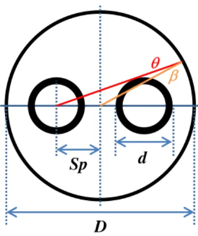
of pipe and the borehole (Figure 1). A model must consider the resistance contributions from the fluid (typically water) flowing inside the two pipes (supply and return joined at the base of the wellbore by a U-bend), through the pipe walls, and through the medium (typically grout) that fills the space between the pipes and surrounding bore wall.

Sp d

D

θ

β

Figure 1. Cross-section geometry of a typical closed-loop heat exchange well. Dimensional parameters

D, d, and Sp refer to the borehole diameter, pipe exterior diameter, and pipe spacing, respectively. The occultation angles θ and β are also shown

Thermal transport within the system may be represented by an equivalent network of resistors (Figure 2), where the temperatures are designated T1, T2, and Tb for the supply and return legs and borehole wall,

respectively. The thermal resistance of each pipe, Rp1 and Rp2, are composed of convection at the inside

wall and conduction through the pipe wall. The shunt resistance, Rs, addresses heat transfer between the

pipes through the medium, while Rb defines the thermal resistance between pipe surfaces to the

surrounding wall.

T

_R

T

p1

R

R

R

R

T

q_{1 q}

2

q₃

Figure 2. Resistance network model representing wellbore heat transfer

The temperature of the elements within the network model are considered unique, such that T1>T2>Tb for

the cooling season and Tb>T2>T1 during heating. The three governing equations that describe the resistive

network are

(

) (

)

(

) (

)

(

)

(

)

3Rs + q +q Rb + q −q Rb =

where q is heat flux. Assuming Rp1 = Rp2 and Rb1 = Rb2 (symmetric case in which pipe is equidistant from

the borehole center), Eq.(1) through (3) may be solved simultaneously assuming steady-state conditions to reveal 3 1 2R T R R T q b p avg ∆ + + ∆ = (4) 3 2 2R T R R T q b p

avg ₋ ∆

+ ∆ = (5) shunt R T

q₃= ∆ (6)

where ∆T = T1 – T2, Tavg = (T1 + T2)/2, ∆Tavg = (Tavg - Tb), R3 = (Rp + Rb) – 2Rb/(Rs/Rb + 2), and Rshunt = (Rp

+ Rb)(Rs/Rb + 2) – 2Rb.

The pipe thermal resistance includes convective heat transfer from the carrier fluid and heat conduction through the pipe wall, defined as

(

)

= (7)

where subscripts o and i denote outside and inside pipe diameters, hcv is the convection coefficient for

water flowing inside the pipe, and kp is the thermal conductivity of the pipe wall.

Thermal transport between the pipes and bore wall must consider the 2-dimensional geometry of the system and the thermal interference, or obscuration, created by the companion pipe. Applying the shape-factor method for 2-dimensional, steady-state heat conduction [8, 9], the thermal resistance between single pipe and borehole wall may be calculated as:

2 2 2

1 1

1

4 cosh

2 2 _{g occ}

D d x Dd R k f π − ⎛ + − ⎞ ⎜ ⎟ ⎝ ⎠

= (8a)

2 2 2

1 2

2

4 cosh

2 2 g occ

D d x Dd R k f π − ⎛ + − ⎞ ⎜ ⎟ ⎝ ⎠

= (8b)

where D is borehole diameter, d is pipe diameter, and kg is the grout thermal conductivity. The variables

x1 and x2 are the distances between the borehole center and center of pipes 1 and 2, respectively. In the

special case where x1 = x2, these parameters are equivalent to pipe spacing, Sp, and the distance between

the pipes is 2Sp.

Equation (8) may be used to simulate a single off-centered pipe conducting to an unobscured surrounding wall. In a two-pipe system, conductive interference increases the net thermal resistance. To address this obscuration effect, an occultation factor, focc, is applied to the equation that considers the spacing and

dimensions of pipes within a cylindrical borehole:

(

)

occ

f = −β π (9)

(

)

θ₌ − ⎛ ⎞

⎜ ⎟

⎜ ₊ ⎟

1 sin

2

d D

β θ_{= +} − ⎛ ⎞

⎜ ⎟

⎝ ⎠ (11)

The final thermal resistance, Rb, may be calculated by

1 2

1 2 2 p b

R R R R

R R

= +

+ (12)

The borehole thermal resistance may be used to calculate the heat transfer efficiency of a wellbore and predict seasonal ground response to an operation geoexchange system.

3. Results and discussion

3.1 Typical wellbore

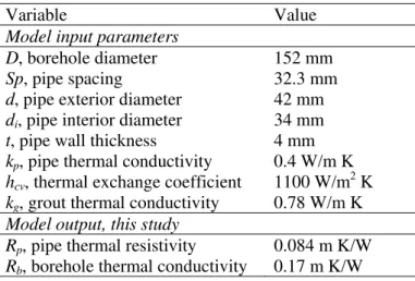
The proposed model was employed to simulate a geoexchange borehole similar to those typically installed in the United States. Common drilling techniques in the US produce a borehole with a diameter of 152 mm (6 inches) filled with a neat bentonite grout with a k of 0.78 W/m K, and round, high density polyethylene (HDPE) tubing with dimensions established in Table 1. In this simulation, the supply and return pipe legs are assumed to be equally-spaced within the borehole, resulting in anSp of 32.3 mm. Applying equations (7) through (12) results in a calculated Rb of 0.17 m K/W.

Table 1. Calculation of thermal resistance for a typical closed-loop borehole

Variable Value

Model input parameters

D, borehole diameter 152 mm

Sp, pipe spacing 32.3 mm

d, pipe exterior diameter 42 mm

di, pipe interior diameter 34 mm

t, pipe wall thickness 4 mm

kp, pipe thermal conductivity 0.4 W/m K

hcv, thermal exchange coefficient 1100 W/m2 K

kg, grout thermal conductivity 0.78 W/m K

Model output, this study

Rp, pipe thermal resistivity 0.084 m K/W

Rb, borehole thermal conductivity 0.17 m K/W

The model was compared to approaches employed by previous studies to validate results (Figure 3). All simulations included the resistive effect of fluid heat transfer and thermal conduction through the pipe wall according to eq. (7). Simulations demonstrate that the proposed model is in general agreement with previous approaches, showing a reduction in Rb as pipe spacing increases. Predicted Rb from eq. (12) is

most similar to (within 5 percent of) the results from Sharqawy et al. [4], who employed a detailed 2-dimensional finite element solution. The Sharqawy et al. study, similar to the current approach, focused on heat transfer through the borehole and assumed a constant temperature boundary condition at the borehole wall. Hellström [6] applied a semi-infinite boundary condition that accounted for a variable thermal field along the borehole perimeter. This results in a predicted Rb that is 14-percent greater than

this study’s approach. Finally, the semi-empirical findings from Remund [1] are 25-percent higher than this study. However, Remund acknowledged his results were higher than predicted by models due to grout voids, uncertainty of pipe placement, and borehole wall irregularities that are inherent in the field.

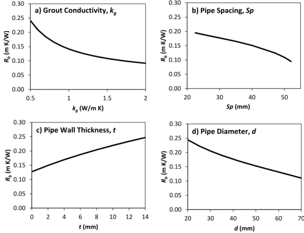
3.2 Sensitivity analysis

Equations (7) through (12) were used to evaluate the causal relationship between the dependent variable

Rb and independent variables kg, Sp, t, and d (Figure 4a, 4b, 4c, and 4d, respectively). All other variables

were consistent with the base case summarized in Table 1. Increasing the thermal conductivity of grout dramatically decreases Rb. However, increasing kg above 1.2 W/m K appears to provide little additional

u-loop. Increasing pipe spacing can reduce Rb by half. Most geothermal boreholes installed in the United

States do not utilize spacers, allowing the pipes to twist which minimizes pipe spacing. We recommend that pipes be pushed against the borehole wall to increase efficiency. Reducing pipe wall thickness improves thermal transfer across the pipe wall. However, reducing t below 3 mm would likely weaken the pipe and cause it to collapse at depth. Another option would be to increase the diameter of the pipe. An increase in pipe diameter increases the surface area and corresponding heat flux. Increasing d is limited by the physical properties of the pipe and the space available within the borehole. The combined benefit of optimizing these parameters yields a significant reduction in Rb. Simulation of the “best

reasonable case” (kg = 1.2 W/m K, Sp = 43 mm, t = 3 mm, and d = 60 mm) reveals an Rb of 0.05 m K/W.

0 0.05 0.1 0.15 0.2 0.25 0.3

0.25 0.3 0.35 0.4 0.45 0.5 0.55 0.6 0.65 0.7

Rb

(m

K

/W)

2Sp/D

This Study Sharqawy Hellstrom Remund

Figure 3. A comparison of effective borehole resistance (Rb) predicted by this study, a finite-element

model (Sharqawy [4]), an semi-infinite analytical model (Hellström [6]), and empirical observations (Remund [1])

0.00 0.05 0.10 0.15 0.20 0.25 0.30

0.5 1 1.5 2

Rb

(m

K/W)

k_g(W/m K)

0.00 0.05 0.10 0.15 0.20 0.25 0.30

20 30 40 50

Rb

(m

K/W)

Sp(mm)

0.00 0.05 0.10 0.15 0.20 0.25 0.30

0 2 4 6 8 10 12 14

Rb

(m

K/W)

t(mm)

0.00 0.05 0.10 0.15 0.20 0.25 0.30

20 30 40 50 60 70

Rb

(m

K/W)

d(mm)

a) Grout Conductivity, k_g b) Pipe Spacing, Sp

c) Pipe Wall Thickness, t _{d) Pipe Diameter,} d

3.3 Importance of Rb

Previous studies have emphasized the importance of minimizing Rb. Comparatively few, however, have

quantified the overall benefit of reducing borehole thermal resistance in cases where heat transfer may be limited by the thermal conductivity of the surrounding geologic medium (kr). To test the relative

importance of Rb, we simulated a borehole using the spatial dimensions in Table 1 with a 2-dimensional

finite difference model[10]. Well efficiency, Ec, was computed by comparing the response of borehole

with resistance Rb to a borehole with zero thermal resistance as a function of kr. Representative values of

Rb ranged from 0 to 0.3 m K/W as suggested by this study. Thermal conductivity was adjusted to

represent coal, limestone, saturated sand, granite, and quartzite (Table 2).

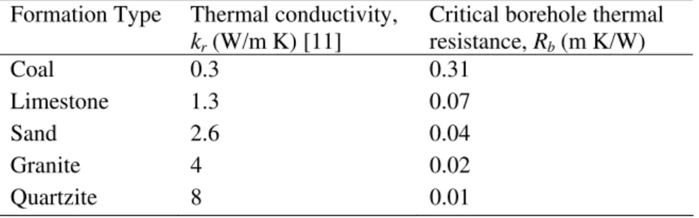
Table 2. Thermal conductivity, kr, and the critical borehole thermal resistance, Rb, for a variety of

representative geologic materials

Formation Type Thermal conductivity,

kr (W/m K) [11]

Critical borehole thermal resistance, Rb (m K/W)

Coal 0.3 0.31

Limestone 1.3 0.07

Sand 2.6 0.04

Granite 4 0.02

Quartzite 8 0.01

Well efficiency diminishes as Rb and kr increase (Figure 5). This results because a geoexchange well

installed within a high-kr formation is more likely to be limited by thermal resistance within the borehole.

A significant (>1 percent) reduction in well efficiency is predicted if Rb increases above a critical value

(column 3 in Table 2). This demonstrates that for most geologic media (with the notable exception of coal), thermal exchange is likely to be limited by borehole thermal resistance. This emphasizes the benefit of reducing Rb under most geologic situations. Moreover, the model shows that improved

construction of the geoexchange piping could improve the overall efficiency of a system installed in typical geologic materials (limestone, sand, and granite) by 10 percent.

The relationship between well efficiency and the product of Rb and kr is well-defined (Figure 5b). For the

typical well geometry investigated by this study, Ec may be calculated from the relation

(aR kb r)

c

E =e (13)

where a = -0.105. This equation fits the simulated data well, with an R2coefficient of 0.9999.

0.75 0.8 0.85 0.9 0.95 1

0 0.1 0.2 0.3

Ec

R_b(m K/W)

Coal, kr = 0.3 W/m K Limestone, kr = 1.3 W/m K Sand kr = 2.6 W/m K Granite kr = 4 W/m K Quartzite kr = 8 W/m K

0 0.1 0.2 0.3 0.4 0.5 0.6 0.7 0.8 0.9 1

0 5 10 15 20

Ec

R_bk_r

Model Simulated

Curve Fit

(a) (b)

Figure 5.Thermal well efficiency (Ec) as a function of borehole thermal resistance (Rb) and the thermal

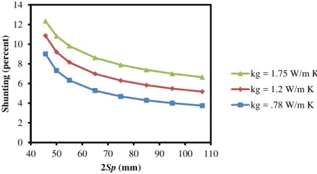
3.4 Shunting

The thermal shunt between the legs of the pipe loop is calculated from eq. (6), where Rs is developed

from the pipe to pipe shape factor analysis in a surrounding cylinder from [8] where:

(

)

1

cosh 2 2 / 1 s

R = − ⎡_⎣ Sp d − ⎤_⎦ (14)

As shown in Figure 6, the loop’s ability to dissipate heat is compromised by the thermal shunt, which exists between supply and return legs of the loop. The vertical axis is a measure of the heat shunted between legs of the loop to the heat applied or extracted at the surface. When the pipes are in close proximity, the shunted heat transfer increases, and the performance of the loop is diminished. Alternatively, when the pipes are spread far apart (contacting the perimeter of the bore wall, for instance), shunting is minimized and the loop performance is maximized. Figure 6 shows that the thermal shunt is exacerbated for close spacing (small Sp) and for larger grout conductivity, kg, while the least

shunting is for legs that are separated widely and for low grout conductivity (i.e., neat bentonite).

0 2 4 6 8 10 12 14

40 50 60 70 80 90 100 110

S

hunt

in

g (p

er

ce

nt

)

2Sp(mm)

kg = 1.75 W/m K kg = 1.2 W/m K kg = .78 W/m K

Figure 6. Loop thermal shunt between legs as function of spacing and grout conductivity

In practice, closely spaced U-bends and installation practices that allow the pipes to twist and contact one another over the pitch of the twist will suffer the consequences of greater thermal shunting. This has the effect of reducing the effective length of the loop, since the applied heat never makes it fully down hole, but instead raises the temperature of the upcoming water, so that (T1-T2), or the effective loop heat

rejection, is smaller than what it would be with no shunting.

4. Conclusions

The analytical solution developed by this study to calculate borehole thermal resistance is computationally efficient, represents a variety of borehole geometries, and is readily accessible to installers because it requires no additional software. The model is particularly useful for predicting the benefits of optimizing borehole geometry and properties of the pipe and grout. The model compares well with previous studies, although actual Rb is likely to be somewhat greater than predicted by any model

due to problems with grouting, pipe placement, and drilling techniques encountered in the field. Previous studies have emphasized the importance of increasing kg as a means of reducing Rb; however, increasing

kg alone may cause unwanted thermal shunting between pipe legs. Numerical simulations demonstrate

that reducing Rb could increase well thermal exchange efficiency by over 10 percent for most geologic

materials. Future efforts to improve performance of geoexchange wells should consider maximizing pipe spacing, pipe surface area, and minimizing pipe wall thickness in addition to increasing kg, which could

significantly improve efficiency.

References

[2] Liao Q., Zhou C., Cui W., and Jen T. Effective borehole thermal resistance of a single u-tube ground heat exchanger. Numerical Heat Transfer 2012, 62, 197-210.

[3] Sagia Z., Stegou A., and Rakopoulos C. Borehole resistance and heat conduction around vertical ground heat exchangers. The Open Chemical Engineering Journal 2012, 6, 32-40.

[4] Sharqawy M.H., Mokheimer E.M., and Hassan M.B. Effective pipe-to-borehole thermal resistance for vertical ground heat exchangers. Geothermics 2009, 38, 271-277.

[5] Gu, Y. and O’Neal, D. Development of an equivalent diameter expression for vertical u-tubes used in ground-coupled heat pumps. ASHRAE Transactions 1998, v. 104, n. 2, 9 p.

[6] Hellström, G. Ground heat storage, thermal analyses of duct storage systems. Doctoral thesis 1991, Department of Mathematical Physics, University of Lund, Lund, Sweden.

[7] Philippe M. Bernier M., Marchio D. Sizing calculation spreadsheet vertical geothermal borefields. ASHRAE Journal 2010, 7, 20-28.

[8] Andrews R.V. Solving conductive heat transfer problems with electrical-analog shape factors, Chemical Engineering Process, 1955, 51(2), 67 p.

[9] Holman J.P. Heat Transfer, Sixth Edition. McGraw-Hill Publishers, New York, NY, 676 p.

[10] Harbaugh, A. Banta, E., Hill, M., and McDonald, M. MODFLOW-2000, the U.S. Geological Survey modular ground-water model. Open-File Report 00-92 2000, U.S. Geological Survey, 121 p.

[11] Banks, D. An Introduction to Thermogeology: Ground Source Heating and Cooling 2008, Blackwell Publishing, Oxford, UK, 339 p.

Albert A. Koenig, PhD physics, Duke University, Durham, North Carolina, USA. VP of American

Refining & Biochemical, Inc. (ARB) and founder of ARB Geowell, LLC. By training and practice, he is a physicist and consulting engineer in the greater Philadelphia area. He has been involved in numerous alternative energy development activities since 1975, including large solar thermal industrial energy projects, residential passive solar and photovoltaic applications, testing of the first 0.5 MWe wind turbine, advanced battery development for EVs, battery energy storage for on-site power, SOFC fuel cells, enhanced oil recovery and geothermal HVAC. Dr. Koenig is a member of the National Ground Water Association (NGWA), the Am. Soc. Of Heating, Refrigeration and Air Conditioning Engineers (ASHRAE), and the Association of Energy Engineers, Greater Philadelphia Chapter.

E-mail address: [email protected]

Martin F. Helmke, PhD Geology and Water Resources, Iowa State University, Ames, Iowa, USA.

Associate Professor of Hydrogeology at West Chester University of Pennsylvania and Director of the Geothermal Research Consortium. Dr. Helmke is the lead investigator advancing the ground-source heat pump conversion of the WCU campus, which is one of the largest geothermal systems in the US. He has published extensively in the fields of heat, groundwater, and contaminant transport through heterogeneous geologic media. Dr. Helmke is a licensed professional geologist in Pennsylvnia. E-mail address: [email protected]