www.atmos-chem-phys.net/11/9395/2011/ doi:10.5194/acp-11-9395-2011
© Author(s) 2011. CC Attribution 3.0 License.
Chemistry
and Physics
Simple kinematic models for the environmental interaction of
tropical cyclones in vertical wind shear
M. Riemer1,*and M. T. Montgomery1,2
1Department of Meteorology, Naval Postgraduate School, Monterey, CA, USA 2NOAA’s Hurricane Research Division, Miami, FL, USA
*current address: Institut f¨ur Physik der Atmosph¨are, Johannes Gutenberg-Universit¨at, Mainz, Germany
Received: 28 August 2010 – Published in Atmos. Chem. Phys. Discuss.: 16 November 2010 Revised: 23 May 2011 – Accepted: 19 August 2011 – Published: 12 September 2011
Abstract. A major impediment to the intensity forecast of tropical cyclones (TCs) is believed to be associated with the interaction of TCs with dry environmental air. However, the conditions under which pronounced TC-environment inter-action takes place are not well understood. As a step towards improving our understanding of this problem, we analyze here the flow topology of a TC immersed in an environment of vertical wind shear in an idealized, three-dimensional, convection-permitting numerical experiment. A set of dis-tinct streamlines, the so-called manifolds, can be identified under the assumptions of steady and layer-wise horizontal flow. The manifolds are shown to divide the flow around the TC into distinct regions.
The manifold structure in our numerical experiment is more complex than the well-known manifold structure of a non-divergent point vortex in uniform background flow. In particular, one manifold spirals inwards and ends in a limit cycle, a meso-scale dividing streamline encompassing the eyewall above the layer of strong inflow associated with sur-face friction and below the outflow layer in the upper tro-posphere. From the perspective of a steady and layer-wise horizontal flow model, the eyewall is well protected from the intrusion of environmental air. In order for the environmental air to intrude into the inner-core convection, time-dependent and/or vertical motions, which are prevalent in the TC inner-core, are necessary. Air with the highest values of moist-entropy resides within the limit cycle. This “moist envelope” is distorted considerably by the imposed vertical wind shear, and the shape of the moist envelope is closely related to the shape of the limit cycle. In a first approximation, the distri-bution of high- and low-θeair around the TC at low to mid-levels is governed by the stirring of convectively modified air by the steady, horizontal flow.
Correspondence to:M. Riemer ([email protected])
Motivated by the results from the idealized numerical ex-periment, an analogue model based on a weakly divergent point vortex in background flow is formulated. The simple kinematic model captures the essence of many salient fea-tures of the manifold structure in the numerical experiment. A regime diagram representing realistic values of TC inten-sity and vertical wind shear can be constructed for the point-vortex model. The results indicate distinct scenarios of en-vironmental interaction depending on the ratio of storm in-tensity and vertical-shear magnitude. Further implications of the new results derived from the manifold analysis for TCs in the real atmosphere are discussed.
1 Tropical cyclone intensity and environmental air interaction
It has long been recognized that the interaction of tropical cy-clones (TCs) with environmental air can have a detrimental effect on storm intensity. The interaction can be expected to be particularly pronounced when vertical shear of the envi-ronmental horizontal wind is present. Vertical wind shear ensures that at some height levels the environmental flow is distinct from the motion of the storm and considerable storm-relative environmental flow arises at such levels (e.g. Willoughby et al., 1984; Marks et al., 1992; Bender, 1997). This storm-relative flow then advects environmental air to-wards the TC. If low moist-entropy (or equivalent potential temperature,θe) air associated with the environment can in-trude into the eyewall updrafts, then the conversion of heat into kinetic energy within the TC’s power machine is frus-trated and the storm can be expected to weaken (Tang and Emanuel, 2010a). Moistening and warming of the environ-mental air before reaching the eyewall updrafts may diminish this detrimental impact on TC intensity.
upon the hurricane heat engine”. Based on an inspection of the storm-relative radial flow at mid-levels (their Fig. 4), they noted “a prominent movement of environmental air through the storm” and suggested that “the vortex wasventilatedby invading colder masses of air”. This ventilation of the TC vortex by storm-relative environmental flow is widely in-voked to explain the intensity evolution of observed storms (e.g. Willoughby et al., 1984; Marks et al., 1992; Shelton and Molinari, 2009). Emanuel et al. (2004) developed an empir-ical parameterization within an axisymmetric model frame-work that attempts to account for the ventilation of low-θe air through the TC core at mid-levels in association with an imposed vertical wind shear1. A somewhat related pathway of environmental interaction in vertical shear was proposed by Frank and Ritchie (2001). In their model, shear-induced eddy fluxes of potential temperature were hypothesized to erode the upper-level warm core, leading to an increase of the minimum surface pressure by hydrostatic arguments, and ultimately to a decrease of TC intensity.
When considering TC-environment interaction it needs to be borne in mind that a mature TC constitutes a strong at-mospheric vortex. This is particularly true when trying to draw conclusions based solely on the storm-relative asym-metricflow, i.e. the storm-relative flow that results after sub-tracting the axisymmetric TC circulation. The asymmetric flow may serve as an approximation for the environmen-tal flow. The storm-relative asymmetric flow has been re-ferred to as “cross-vortex flow” (Willoughby et al., 1984; Black et al., 2002) or there has been the tacit assumption that air flowsthroughthe inner core (Simpson and Riehl, 1958; Bender, 1997; Zhang and Kieu, 2006). The strong swirling winds, however, act to significantly deflect the storm-relative asymmetric flow2. Air parcel trajectories in a mature TC, of course, differ greatly from the streamlines of the storm-relative asymmetric flow. This distinction does not always seem to be clear in a number of previous studies. Only for relatively weak storms and strong storm-relative envi-ronmental flow does it seem plausible that envienvi-ronmental air will actually penetrate the eyewall of a TC (e.g. Hurricane Claudette (2003), Shelton and Molinari, 2009). The focus of this paper is to explore the limitations of vortex-environment interaction based on the above kinematic considerations.
The foregoing ideas hint that a more efficient way to ingest dry environmental air into the eyewall updrafts is through the storm’s inflow layer. In the current study, the term “in-flow layer” will refer to the layer of strong in“in-flow associated
1This empirical parameterization is now used each hurricane
season in the CHIPS forecast model of Kerry Emanuel.
2The strong radial shear of the swirling winds tends also to damp
any asymmetry that tries to invade the TC. This is the so-called vortex axisymmetrization process (e.g. Melander et al., 1987; Carr and Williams, 1989) that is a well-known essential ingredient in the robustness and persistence of coherent vortex structures in quasi two-dimensional flows. The axisymmetrization process will not be considered explicitly in this study.
with surface friction in the lowest 1 km–1.5 km where the de-parture from gradient wind balance in the radial direction is generally a maximum (e.g., Bui et al. (2009), Figs. 5 and 6 and accompanying discussion). Riemer et al. (2010, RMN hereafter) have shown how the interaction of vertical shear with a mature TC can form persistent, vortex-scale down-drafts which flush the inflow layer with low-θeair and effec-tively reduce eyewallθe values by 3 K to 9 K, depending on the magnitude of vertical shear. Without explicit considera-tion of vertical shear effects, earlier studies have shown that downdrafts associated with individual rain bands may bring low-θeair into the inflow layer (Barnes et al., 1983; Powell, 1990). Powell has estimated that the replenishment of this air by surface fluxes may not be complete before reaching the eyewall and concluded that this process could affect the intensity evolution of the storm. In a more recent model-ing study, Kimball (2006) has found that “dry environmen-tal air above approximately 850 hPa rotates cyclonically and inward around the storm center” and may be subsequently involved in downdrafts close to the eyewall. Two schematic diagrams summarizing how the TC power-machine may be frustrated by mid-level ventilation and pronounced down-drafts are given in Figs. 1 and 2 of RMN.
The processes discussed above, the ventilation of eyewall convection, the erosion of the upper-level warm core, and the depression of inflow layerθe by downdrafts, are widely believed to operate in real storms3. The relative importance of these processes for intensity modification is generally un-known and the environmental conditions under which they may operate are not well understood. This is consistent with the fact that the interaction with vertical shear and/or the presence of dry air in the vicinity of a storm poses an en-hanced forecast challenge. Dry air can be observed to im-pingeon TCs (e.g. Zipser et al., 2009, tropical storm Debby), yet it has not been entirely clear how storm intensity is af-fected. Idealized experiments demonstrate that dry air may wrap all around a developing TC in quiescent environment without affecting storm intensity at all (S. A. Braun, personal communication, 2010). Similar questions arise for TCs that interact with the Saharan air layer (SAL)4.
Aspects of TC-environment interaction have received con-siderable attention on the convective scale and the scale of individual rain bands (e.g. The Hurricane Rainband and In-tensity Change Experiment, Houze et al., 2006). However, we believe that an overarching framework for this problem is still lacking. The goal of the present study is to contribute
3A kinematic impact on TC intensity for a sheared storm arises
through vortex tilt, i.e. the vertical misalignment of the TC’s poten-tial vorticity tower. However, as discussed in the introduction of RMN, there is strong indication that this kinematic effect is not a primary intensity change mechanism.
4The effect of SAL, however, is thought to be more complex
to such a framework by taking a broader-scale viewpoint and considering the larger-scale air mass distribution around a TC.
1.1 Revisiting a horizontal and steady flow model
For steady, two-dimensional flow, the flow topology can be examined by analyzing the hyperbolic fixed points and their associated manifolds. At a fixed point, both horizontal wind components vanish. A fixed point is hyperbolic when air parcels in the vicinity of this point are stretched in one di-rection and contracted in another didi-rection. Mathematically speaking, when the flow field is linearized around a hyper-bolic fixed point, the eigenvalues of the strain tensor are real and of opposite sign. Here, we will refer to hyperbolic fixed points simply as stagnation points. Streamlines that emanate from a stagnation point constitute the hyperbolic manifolds of the flow. A manifold along which the flow approaches the stagnation point is called a stable manifold. A mani-fold along which the flow departs from the stagnation point is called an unstable manifold. Hyperbolic manifolds divide the flow into different regimes and thus determine the topology of the flow. Note that the identification of stagnation points is crucial for the objective analysis of the flow topology.
For steady, non-divergent flow the interaction of a vortex with the background flow gives rise to a manifold that sep-arates the area of rotation-dominated flow from the larger-scale environment. For this special case, we refer to the man-ifold as a dividing streamline. Inside of the dividing stream-line, all streamlines are closed and air parcels are confined to the vortex. Outside the dividing streamline, the flow passes around the vortex. The stagnation point in this example is found where the velocity field of the vortex and that of the background flow cancel.
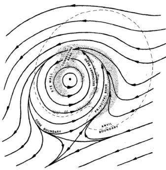
Based on this basic fluid-dynamical concept, Willoughby et al. (1984, hereafter WMF84) proposed that for a TC in storm-relative environmental flow ”the streamline pattern is divided into a vortex core where the streamlines form a closed gyre and the vortex envelope where they curve around the core in a wavelike pattern” (Fig. 1). These authors noted further that “in the closed gyre, the air moves with the vortex; in the envelope, environmental air passes through the vortex and around the core”. Willoughby et al. noted clearly the existence and importance of flow boundaries in the vicinity of a vertically sheared TC. These authors indicated also that the air within the closed gyre has generally higherθevalues than outside of the gyre.
WMF84’s seminal hypothesis of separated flow regions with distinct thermodynamic properties and its ramifications for the interaction of TCs with environmental air have re-ceived little attention in the literature. WMF84’s results are derived from a low wave-number analysis of observational data from a number of flight legs within 150 km of the storm center. Most notably, the stagnation point was not contained within the domain considered by WMF84. We believe that
Fig. 1. Willoughby et al.’s hypothesized flow topology of a ma-ture TC in northeasterly storm-relative flow above the inflow layer (approx. 850 hPa, their Fig. 18). The closed gyre around the center is supposed to contain the moist “vortex air” while drier environ-mental air is found outside the dividing streamline. The shading indicates regions of deep convection. The principal, secondary, and connecting band constitute the so-called stationary band complex.
it is worthwhile to revisit WMF84’s seminal hypothesis and analyze the flow topology of a TC in vertical wind shear with a much more complete data set from a recent idealized nu-merical experiment.
also. Thus, we believe that the steady-flow approximation provides scientific value for studying TC-environment inter-action in the real atmosphere.
In the vicinity of the eyewall, however, the assumptions of steady and layer-wise horizontal flow break down. In a mature TC, vortex Rossby waves (VRWs) and their cou-pling to convection and the boundary layer are arguably the most important transient flow features in this region (Mont-gomery and Kallenbach, 1997; Chen and Yau, 2001; Wang, 2002; Chen et al., 2003). For an intensifying TC, rotating deep convective structures, also referred to as “vortical hot towers”, can be expected to be dominant features (Nguyen et al., 2008). This rich fluid dynamical behavior is not con-sidered here. An extensive trajectory analysis of the time-dependent, three-dimensional flow to quantify the mid-level ventilation of eyewall convection in a numerical simulation of Hurricane Bonnie (1998) has been performed by Cram et al. (2007). The analyses therein were limited to a 5 h time-scale for back trajectories and confined to a 100 km radius from the center of the vortex. That study also did not con-sider the broader-scale interactions between the environment and the inner-core region.
A natural extension of the current study is to examine the Lagrangian coherent structures (LCS) that govern the inter-action of fluid from distinct regions in the unsteady, three-dimensional flow (e.g. Haller, 2001). These LCS are the finite-time manifolds of the time-dependent flow. First anal-yses of such LCS in TCs have recently been performed by Sapsis and Haller (2009) and Rutherford et al. (2010). We anticipate that the analysis of LCS in a vertically sheared TC will yield further insight into the interaction of the TC with environmental air. The current study nonetheless should pro-vide a useful framework for interpreting the results from an analysis of the LCS.
An outline for the paper is as follows. In Sect. 2 we use the idealized numerical experiment of RMN to illustrate the flow topology and its relation to distinct air masses around the ver-tically sheared TC. Motivated by the model results we then formulate an analogue model based on a point vortex with singular mass sink in Sect. 3. The analogue model is shown to capture the basic features of the flow topology in the ideal-ized numerical experiment. Section 4 considers application of the analogue model to the problem of TC-environment in-teraction in the real atmosphere. Conclusions are presented in Sect. 5.
2 Flow topology in an idealized numerical experiment of TC-shear interaction
We analyze the flow topology of a mature TC in an idealized numerical experiment. The experiment analyzed herein is the 15 mps case of RMN. The Regional Atmospheric Mod-eling System (RAMS, Pielke et al., 1992; Cotton et al., 2003) was used to perform this experiment. We have deliberately
employed a very simple set of parametrizations, most impor-tantly a bulk aerodynamic formulation for the surface fluxes and warm-rain microphysics. For a detailed description of the RAMS and the experimental setup the reader is referred to RMN. Our experiment considers a TC that has been spun up in quiescent environment on an f-plane for 48 h. After this time the TC has reached an intensity5of 68 ms−1and is sud-denly exposed to a zonal wind profile with vertical shear. The zonal wind profile has a cosine structure in the vertical with zero winds at the surface and 15 ms−1 easterlies at 12 km and above. After the environmental vertical shear flow is im-posed, the TC starts moving to the west, with a small south-ward component, with an approximate translation speed of 5 ms−1.
Distinct changes in the TC structure occur a few hours af-ter shear is imposed. The structural changes and their impor-tant connection to the thermodynamic impact on the TC in-flow layer have been examined in detail in RMN. In response to the vertical shear forcing the TC vortex settles quickly into a quasi-equilibrium tilt direction approx. 90◦left of the shear vector6. Such a tilt equilibrium may be achieved when the cyclonic precession of the tilted vortex cancels the differen-tial advection by the vertical shear flow (Jones, 1995; Reasor et al., 2004). The vorticity anomaly associated with the tilt of the outer vortex at low levels contributes to the formation of a pronounced convective asymmetry outside of the eyewall, reminiscent of the stationary band complex (SBC) defined by WMF84. The SBC extends outwards up to a radius of approx. 180 km and wraps from the downshear-right at low levels to the downshear to downshear-left quadrants at upper levels. Strong and persistent, vortex-scale downdrafts form underneath the helical SBC updrafts. These downdrafts flush the inflow layer with low-θe air in the downshear-left semi-circle. RMN argue that, to first order, it is this flushing of the inflow layer with lowθethat governs the intensity evolution of the vertically sheared TC. While the TC in the reference run without vertical wind shear continues to intensify rapidly, the intensity of the TC in the 15 mps case remains approxi-mately constant in the first 8–10 h after the shear is imposed. With ongoing flushing of low-θeair into the inflow layer, TC intensity decreases by 10 ms−1in the subsequent 6–8 h. As-sociated with a gradual recovery of the inflow layerθe, the TC then starts to re-intensify.
2.1 Analyzed flow structure
The correct frame of reference is of immanent importance for the analysis of the Lagrangian flow structure under the as-sumption of steady flow (see, e.g., Fig. 3 of Dunkerton et al., 2009 and the accompanying discussion on p. 5624–5625). In our case, this is the frame of reference moving with the
5In RMN and in this study, intensity is defined as the maximum
azimuthal mean tangential wind at 1 km height.
6In RMN, the tilt is defined as the vector difference between the
mature storm. We thus use data in a storm-relative frame of reference. A square domain of 2450 km side length cen-tered on the TC7is considered, using data from the innermost grid (5 km resolution) where available and from the outer do-mains (15 km and 45 km resolution, respectively) elsewhere. As discussed in the introduction, for the purposes of this in-vestigation the flow outside the inner core in the numerical experiment can be meaningfully approximated as steady for
O(1 day). This steady flow is represented here by a 6 h time
average over the period from 3–8 h after the shear was im-posed.
The algorithm of Ide et al. (2002) is applied to linearize the velocity field in the vicinity of the stagnation point and to determine the location of the stagnation point. The stable (unstable) manifolds are found by backward (forward) inte-gration of the steady, layer-wise horizontal velocity field, us-ing a second-order Runge-Kutta scheme with a spatial incre-ment of 2.5 km. The manifolds are seeded along the eigendi-rections of the linearized velocity field at a distance of 1 grid point (5 km) from the stagnation point.
2.1.1 Overview
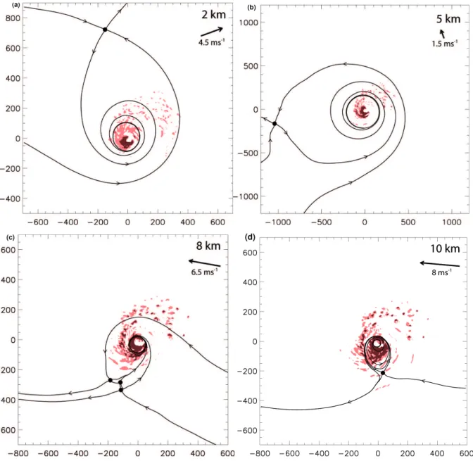
We first provide an overview of the flow topology before ex-amining its relation to the distribution of high- and low-θe air in the vicinity of the TC. The flow topology at low-levels above the inflow layer (z=2 km), at mid-levels (z=5 km), at upper-levels (z=8 km), and just below the outflow layer (z=10 km) will be considered in the following. The radial profiles of the azimuthally averaged tangential winds at these levels are shown in Fig. 2. As can be expected, the max-imum tangential winds, as well as the tangential winds at outer radii, decrease with height. The shape of the radial profile is similar at all 4 levels.
The storm-relative environmental flow, calculated as the average storm-relative flow between radii of 200 km and 1000 km, is 4.5 ms−1 from approx. west at 2 km, 1.5 ms−1 from approx. south at 5 km, and 6.5 ms−1 and 8 ms−1 from approx. east at 8 km and 10 km, respectively. The storm-relative environmental flow changes direction by ap-prox. 180◦between low- and upper-levels and is minimized at mid-level which is characteristic of a vertical shear pro-file with a vertical wave number 1 structure. The strength of the tangential flow and the magnitude of the storm-relative flow at 2 km height in our numerical experiment is com-parable to one of the cases considered by WMF84 (Hurri-cane David (1979), their Fig. 2), except for the direction of the storm-relative environmental flow. As mentioned by WMF84, the flow topology can be reoriented to adjust for this difference.
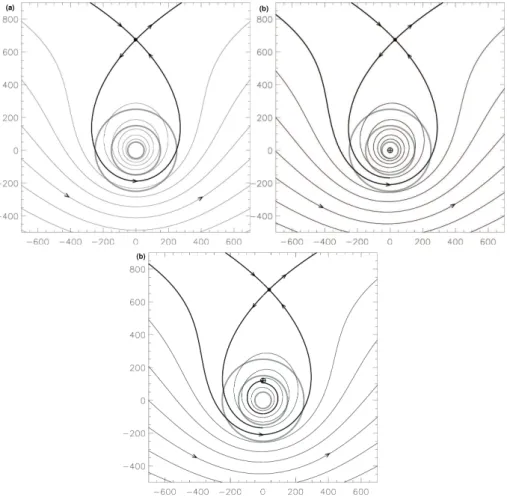
The flow topology in our experiment and its vertical struc-ture are shown in Fig. 3. The flow topology in WMF84’s
7The TC center is defined as the centroid of vorticity averaged
over the lowest 2 km in a square with a side length of 120 km around the surface pressure minimum.
Fig. 2. Azimuthally averaged radial profiles of tangential winds for the no shear case of RMN at 2 km (solid), 5 km (dotted), 8 km (dashed), and 10 km (dash-dotted), averaged over a 6 h period after 48 h of spin up. These profiles represent the TC wind structure at the time at which shear is imposed. For comparison, the profile for the Cat1 point vortex (red, see Sect. 3.2.1) is shown outside of 50 km.
schematic (Fig. 1) was derived from winds at 850 hPa and is thus comparable to our results at 2 km height (Fig. 3a). The signature and location of the SBC in the schematic of WMF84 was derived from radar reflectivities and satellite imagery and is thus more representative of vertical motion at mid- to upper levels (e.g. at 5 km and 8 km in our Fig. 3) than of the low-level vertical motion at 2 km height. After reorientation of WMF84’s schematic by 180◦ to adjust for the differences in the direction of the storm-relative environ-mental flow, a comparison with our results at 2 km height (Fig. 3a) reveals some notable differences. The stagnation point is found at a radius of approx. 700 km in our case, con-siderably farther outside than hypothesized by WMF84. One unstable manifold spirals inwards because the flow is weakly convergent at this level. This manifold ends in a so-called limit cycle, a closed streamline encompassing the strong up-drafts in the inner core. In this case, the limit cycle is analo-gous to the closed streamline that encompasses the inner core and contains the “vortex air” in WMF84’s hypothesized flow topology. In contrast, the outer portion of the manifolds are located at a considerably larger radius. These differences can be expected to be less pronounced for less intense TCs (see Eq. (13) below).
Fig. 3.Stagnation points (black dots) and manifolds at 2 km(a), 5 km(b), 8 km(c), and 10 km(d)height. The eyewall updrafts are indicated by the dark red shading (1 ms−1), light red shading denotes vertical motion of 0.25 ms−1. The magnitude and direction of the storm-relative flow is given in the upper-right of each panel. The values are rounded to 0.5 ms−1. The storm-relative environmental flow is calculated as the averaged flow between 200 km and 1000 km radius. The storm-relative asymmetric flow in this region is essentially uniform (not shown). All fields are from the 15 mps run of RMN and averaged from 3–8 h. The horizontal scale is in km; note the larger scale at 5 km height in(b).
at 2 km height. Consistent with storm-relative flow from the south, the stagnation point is located to the west. The inner core is encompassed by a large limit cycle of approx. 150 km radius. At 8 km and 10 km height, the stagnation points are located to the south and within 200 km–300 km from the cen-ter. Again, the location of the stagnation points is consistent with the direction and the stronger magnitude of the storm-relative environmental flow, and the weaker swirling winds at these levels as compared to 2 km and 5 km height. At 8 km height the limit cycle just encloses the eyewall updrafts. At
10 km height, the manifolds form a virtually closed stream-line that contains the eyewall.
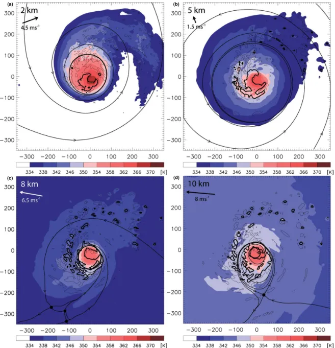
Fig. 4.Zoomed-in version of Fig. 3, includingθe(color shaded) and vertical motion (thin contour = 0.25 ms−1, thick contour = 1 ms−1).
The analyzed flow topology is virtually identical when time averages from 2–7 h and 4–9 h, respectively, are used. The general characteristics of the flow topology shown in Fig. 3 are also found for the 6 h periods from 10–15 h and 16–21 h. The temporal differences in the details of the flow topology are discussed in Sect. 2.1.3.
2.1.2 The meso-scale environment of the eyewall
A zoomed-in version of Fig. 3, overlaid with θe (Bolton, 1980) at each respective height level, is shown in Fig. 4. A striking feature is that the distribution ofθeis closely related
to the manifold structure above the inflow layer up to 10 km height. Air with the highest values ofθeare contained within the limit cycle8(2 km–8 km height) or within the effectively closed streamline at 10 km height.
At 2 km height a clear wave number 1 asymmetry in the θe distribution is found (Fig. 4a). Very low values ofθeare found within a radius of 100 km south of the center. To the north of the center, high values ofθe are found within the
8The limit cycle is a robust feature of the flow topology derived
limit cycle and the innermost spiral, extending to a radius of 150 km. In contrast, at 5 km height theθedistribution in the inner core is approximately symmetric, consistent with the shape and location of the limit cycle at this level (Fig. 4b). At 8 km, the highestθevalues outside of the eyewall are found southwest of the center, approximately bounded by the man-ifolds. At 10 km, air withθe values of 342 K and lower ap-pears to approach the TC from upshear. The eyewall and the highestθe values, however, are still encompassed by the closed streamline. The vertical motion field indicates that up-drafts within the SBC provide higherθeair from below that is then advected to the downshear side with the quasi-steady flow.
Sinceθetends to be a materially conserved quantity above the surface layer,θeis an approximate invariant of the time-dependent, three-dimensional flow. Figure 4 shows a high degree of congruence between theθeisopleths and the man-ifolds of the steady, horizontal flow, in particular at low to mid-levels. Based on this notion we conclude that the shape and location of the moist envelope, i.e. the distribution of high- and low-θe air around the TC, is governed to first or-der by the stirring of convectively modified air by the steady, horizontal flow.
The existence of a closed streamline encompassing the eyewall clearly shows that the eyewall is well protected from the intrusion of environmental low-θ air by the steady, hor-izontal flow. In order for the environmental air to intrude into the inner core convection, time-dependent and/or verti-cal motions are needed. At upper-levels (8 km and 10 km), the manifolds barely encompasses the eyewall. This close approach of the manifolds to the eyewall indicates a poten-tial “hot spot” for the interaction of the eyewall updrafts with environmental air. Note, however, that the highestθe val-ues are well contained within the limit cycle. In particular, there is no indication that the eyewall “leaks”, i.e. that high-θe air is consistently transported downshear from out of the eyewall. Furthermore, from the perspective of the simplified Carnot-cycle model, the impact of ventilation on TC inten-sity is weighted by the difference between the outflow tem-perature and the temtem-perature at the ventilation level. Venti-lation at upper levels is thus not very effective in decreasing TC intensity (Tang and Emanuel, 2010b). In the following we therefore focus on the interaction of environmental air at low- to mid-levels.
2.1.3 Time consistency
The details of the flow topology exhibit some variability for the 6 h time-averaged periods from 10–15 h and 16–21 h. For the sake of brevity we do not present the respective figures but provide a brief description of the salient features.
For the 6 h period from 10–15 h the unstable manifold spi-rals inwards very slowly at 2 km height and ends in a limit cycle that is larger than in Fig. 4a. This larger limit cycle encompasses all of theθe air with values larger than 342 K.
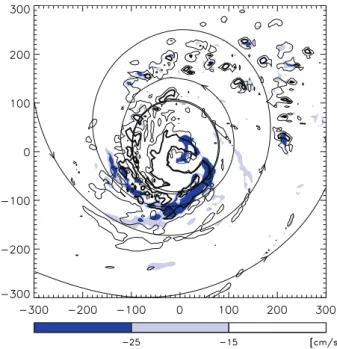
Fig. 5. Downdrafts (colored) and flow topology at 2 km and up-drafts at 8 km (contours, thin = 0.25 ms−1, thick = 1 ms−1). Note that the limit cycle appears as a “thick contour” also because the manifold is plotted several times in a very similar location. The horizontal scale is in km.
At 5 km height there is no stagnation point found within the domain under consideration. This is plausible because the steering level of the TC is expected to be around 5 km height. The storm-relative environmental flow is small at this height and consequently the stagnation point located at a very large radius (Eq. 13). At 8 km height, two stagnation points are found, located in the same region as shown in Fig. 3c. From each of these stagnation points one unstable manifold spirals around the storm center once before reaching the limit cy-cle. At 10 km height, the flow is weakly convergent at this time. Three stagnation points are analyzed from which 2 unstable manifolds spiral around the center. One manifold reaches the limit cycle encompassing the eyewall directly while the other spirals around the center once before merg-ing into the limit cycle. The stable manifolds encompass the eyewall approx. 50 km further outside than during the period from 3–8 h.
For the 6 h period from 16–21 h the flow topology at the individual levels is again very similar as during the period from 3–8 h, except at 5 km height. There, the unstable mani-fold spirals slowly inwards and merges into a limit cycle with a radius of approx. 60 km.
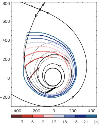
Fig. 6. Backward trajectories at 2 km seeded along a line segment (thick black line south of the center) approximating the central area of the downdraft region shown in Fig. 5. The colors denote the time it takes to reach the downdraft region. The thin lines exemplify some individual streamlines. The horizontal scale is in km.
steady flow appears to be justified and the interpretation of the flow topology in terms of distinct streamlines is physi-cally meaningful.
2.2 Feeding of downdrafts by environmental air
As discussed in RMN, persistent, vortex-scale downdrafts form in the downshear to downshear-left quadrant where pre-cipitation from the helical SBC updrafts falls into the unsat-urated air below. Further insight into the formation of these downdrafts can be obtained by examining the flow topology. Figure 5 indicates that the majority of the downdrafts occur outside of the limit cycle in a region of very lowθeair at 2 km height (see Fig. 4a).
The manifold structure andθedistribution in Fig. 4a indi-cates that the downdraft region is continuously fed with very low θe air from the environment. This flow configuration appears to have two important ramifications. Thecontinuous supply of dry, environmental air prevents the saturation of the air in the downdraft region due to the evaporation of precipi-tation. It is therefore plausible that the downdraft pattern may persist as a quasi-steadyfeature. Secondly, the flow pattern indicates that the environmental air reaches the downdraft
re-gion with very little thermodynamic modification. Evapora-tion of precipitaEvapora-tion from the SBC may thus occur invery dry air, leading to the formation ofparticularly vigorous down-drafts and an associated pronounced depression of the inflow layerθe.
2.3 Origin of environmental air fed into downdrafts
The manifolds of the steady flow identify distinct flow re-gions and their interaction in the limit of long time scales. For the time scale relevant for TC-environment interaction ofO(1 day) only subregions of the flow domain will be
in-volved in such interaction. The extent of these subregions depend on the structure and magnitude of the velocity field. To estimate the origin of the air that is fed into the region of persistent downdrafts we calculate backward trajectories of the steady flow. Note that this steady flow here is represented by a 6 h time average. The backward trajectories are seeded at 2 km height along a line segment to the south of the storm center that approximates the central area of the downdraft re-gion (Fig. 6). The color coding in Fig. 6 denotes where the air parcels are located at 3 h, 6 h, 9 h, ... before reaching the line segment.
Figure 6 illustrates that the source region of the envi-ronmental air that feeds the downdraft area exhibits a pro-nounced asymmetric, azimuthal wave number 1 structure. For the first 12 h, the air originates almost exclusively from the west and north of the model TC. Subsequently, air pro-gressively reaches the downdraft region that has spiraled around the center once. Ultimately, this air has its origin west of the TC also, as can readily be inferred from the manifold structure. For the first 24 h, the source region of air inter-acting with the downdraft region from the south and east of the center is confined to a small radial area (approx. 150 km– 200 km). This radial area is considerably smaller than indi-cated by the stable manifold, which is loindi-cated at a radius of approx. 300 km south and east of the center. The potential ramification of this pronounced asymmetry of the source re-gion of environmental air on TC intensity will be discussed in Sect. 4.3.
3 A potential-flow model for TC-environment interaction
considered previously to examine the interaction of TCs with their environment.
3.1 A convergent point vortex immersed in a uniform background flow
We first consider a mass sink that is co-located with the point vortex.
3.1.1 Streamfunction and wind components
Consider first a point vortex at the origin0with circulationŴ in a polar coordinate system with position vectorx=(r,φ), whereφincreases in the anti-clockwise direction. The verti-cal vorticity is then given by
ζ (x)=Ŵδ(x), (1) where δ(x) is the two-dimensional Dirac delta function. The well-known associated streamfunction in the horizontal plane is
9v(r,φ)= Ŵ
2πlnr, (2)
and the tangential wind vv=
∂9v ∂r =
Ŵ
2π r, (3)
with correspondingly zero radial wind.
Now, instead, consider a point mass sink of strengthDat the origin. This mass sink has divergence
D(x)=Dδ(x). (4) Because the flow associated with this mass sink is every-where non-divergent save for this singularity, the following streamfunction can be defined9:
9div(r,φ)= −
D
2πφ. (5)
Because of our desire to readily visualize the flow, we prefer the use of a streamfunction over the velocity potential. The associated radial wind
udiv= −
∂9div
r∂φ = D
2π r. (6)
The tangential velocity is identically zero. Hereafter, we will absorb the 2π into the definitions ofŴ andD, viz.,Ŵ∗=
Ŵ/2πandD∗=D/2π, and drop the∗notation.
Since the problem of a point vortex in uniform background flow is invariant under (static) rotation we are free to choose the direction of U. We choose the background flow to be zonal and defineφ=0 to be south. Let positiveU denote westerly flow. Cyclonic and outward flow with respect to the
9The streamfunction is a multi-valued function for which the
Riemann sheets connect at 0/2π.
origin is defined to be positive. The streamfunction associ-ated with the background flow is then
9bg(r,φ)=U rcosφ (7)
and the tangential and radial wind components, respectively, are given by
vbg=Ucosφ (8)
and
ubg=Usinφ. (9)
3.1.2 Total streamfunction and flow visualization
Because potential flow satisfies the linear Laplace equation ∇29=0 outside of flow singularities we may superpose the individual solutions. The total streamfunction for a divergent point vortex at the origin immersed in uniform background flow is then:
9(r,φ)=9v+9div+9bg=Ŵlnr−Dφ+U rcosφ. (10)
It is clear from this equation that the term associated with the mass sink (9div) introduces a jump discontinuity10of
magni-tude 2π D when a streamline crosses the southern semi-axis at 0/2π. The streamfunction is therefore multi-valued. Still, Eq. (10) is meaningful to represent the flow field because it is differentiable and thus the wind field is unique. The hyper-bolic manifolds and the streamlines of the flow can be readily visualized when one contour line is chosen to pass through the stagnation point and a contour interval of 2π D, or an in-teger fraction thereof, is used (Fig. 7).
3.2 “TC-like” vortex strength and mass sink
In this subsection we use observations and our idealized nu-merical experiments to give a range of values forŴandD that best represent a TC in the point vortex framework. 3.2.1 Tangential flow
The tangential wind of the point vortex decreases asr−1. It is well known that the radial decrease of tangential winds in mature TCs,vTC, outside of the radius of maximum winds
(RMW) is generally less thanr−1. A reasonable estimate of this radial structure is
vTC=I0r−γ, (11)
withγranging between 0.4 and 0.7 (Mallen et al., 2005, and references therein), andI0 is a constant denoting the storm 10The structure of the equation for the velocity potential8of the
Fig. 7. (a)Streamlines of a stationary, cyclonic, non-divergent point vortex with a circulation of 33.7×10⁵m2s−1(Cat3, see Table 1) in 5 ms−1westerly background flow. The strength of the vortex and the storm-relative environmental flow are chosen to be similar to the idealized numerical experiment at 2 km height (cf. Fig. 3). The streamlines passing through the stagnation point (black dot), the flow’s manifolds, are highlighted. The horizontal scale is in km. The gray concentric circles denote radii 50 km, 150 km, and 250 km, respectively.
(b)Same as(a)but for a weakly convergent point vortex withD= −1.5×10⁵m2s−1. The mass sink is marked by the crossed circle.(c)
Same as(b), but for a mass sink that is displaced 120 km to the north of the center. The emerging closed streamline, reminiscent of the limit cycle found in the idealized numerical experiment (cf. Fig. 3), is highlighted.
intensity. Much of the variability ofγ is believed to be as-sociated with the stage of the TC life cycle11. In general, the radial decay ofvTCis slowest for storms at minimal
hur-ricane strength or weaker. The radial decrease of tangen-tial winds is somewhat steeper at upper-levels (Mallen et al., 2005). Due to the different radial profiles it can be expected that the details of the flow topology of a point vortex and a TC in background flow vary accordingly.
To investigate the general flow topology of the simple point vortex model in the context of TC-environment inter-action, we believe that it is a reasonable choice to define the strength of the point vortex by its tangential winds at 150 km. As is shown below (Sect. 3.3.1) this radius lies in between
11There is some variability ofγwith radius also, consistent with
the well-known fact that the inner and outer wind fields can develop rather independently (Weatherford and Gray, 1988).
the radius of the stagnation point and the closest approach of the dividing streamline to the vortex center, except for strong vortices. Therefore, this choice appears to be a good compro-mise between underestimating the winds at larger radii and overestimating them at small radii. Accordingly, the associ-ated circulation of the point vortex will be denoted byŴ150.
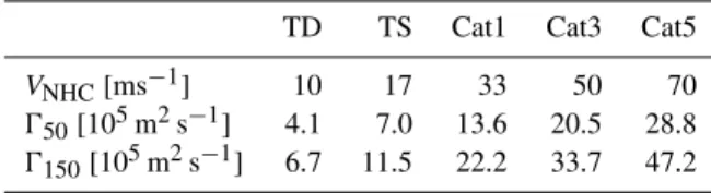
The circulation of several vortices is defined to represent different TC intensities by the following procedure. We spec-ify the maximum wind speed according to the National Hur-ricane Center (NHC) for a tropical depression12, tropical storm, and category 1, category 3, and category 5 hurricanes (Table 1). The corresponding point vortices are referred to as TD, TS, Cat1, Cat3, and Cat5, respectively. The RMW
12There is no official minimum wind speed requirement for the
Table 1.Definition of model vortices based on NHC TC intensity.
TD TS Cat1 Cat3 Cat5
VNHC[ms−1] 10 17 33 50 70 Ŵ50[105m2s−1] 4.1 7.0 13.6 20.5 28.8 Ŵ150[105m2s−1] 6.7 11.5 22.2 33.7 47.2
is set to 35 km13. We use Eq. (11) withγ=0.55 to calcu-late the tangential wind speed at 150 km. This wind speed is then used in Eq. (3) to calculate the circulationŴ150for the
individual vortex. Compared to the generic TC profile with γ=0.55, the point vortex overestimates the winds at 50 km by 64 % and underestimates the winds at 500 km by 42 %. A comparison of the point vortex profile with the radial pro-file of the tangential winds in our numerical experiment is provided in Fig. 2.
To estimate whether environmental air may reach the eye-wall, the overestimation of the tangential wind speed at the radius representing the eyewall is clearly problematic. For this estimate we consider the representation of the different TC categories by a modified circulation,Ŵ50, also. To
cal-culateŴ50, the above procedure is repeated with the winds
of the point vortex matched to the TC profile at a radius of 50 km, instead of 150 km. For theŴ50vortices, the approach
of environmental air is likely overestimated because of the steeper radial wind profile of the point vortex as compared to the TC profile. Below,Ŵrefers toŴ150unless otherwise
noted.
The circulation of the point vortex may represent a TC of specified intensity up to mid-levels, around 5 km. At upper-levels the tangential winds are considerably weaker. In conjunction with the faster radial decay of the wind speed (see above) the closest approach of environmental air to the core region can be expected at upper-levels below the out-flow layer, consistent with the numerical results presented in Sect. 2.
3.2.2 Radial flow
The radial profile of the radial wind above the inflow layer is more variable and less documented observationally than the radial profile of the tangential winds. In this study, we use data from our previously published idealized numerical experiments (i.e., the no shear, 15 mps, and 20 mps case of RMN) to estimate values for D. We consider the tempo-ral average from 4–9 h. For all three experiments the radial flow at 150 km is approx. 1 ms−1which, according to Eq. (6), yields a value ofD= −1.5×10⁵m2s−1for the point vortex model. At 50 km, this value ofDyields a radial inflow ve-locity of 3 ms−1.
13This value underestimates the RMW for tropical depressions
and potentially for tropical storms.
It needs to be pointed out, however, that the radial profiles of the TC in the idealized numerical experiments are not con-sistent with a point mass sink. For all three experiments the radial inflow doesnotincrease inside 150 km. In the no shear and 15 mps case a radialoutflowof 5 ms−1is found at 50 km. There is considerable uncertainty associated with our choice ofD. Nevertheless, the results of our analysis will be shown below to be only weakly sensitive to the choice ofDover a range of reasonable values.
3.3 Flow topology
Without loss of generality, we consider a cyclonic vortex (Ŵ >0)in westerly background flow(U >0).
3.3.1 Non-divergent point vortex
By definition, the stagnation point(rsp,φsp)is found where
both the tangential and radial flow components vanish. The radial flow for the non-divergent vortex vanishes everywhere. The radial component of the westerly background flow van-ishes for φ=0 andφ=π, i.e. due south and due north of the center (Eq. 9). For a cyclonic vortex in westerly back-ground flow the stagnation point is located to the north14, i.e.φsp=π. The condition for the cancellation of the
tan-gential flow is
vv(rsp,φsp)+vbg(rsp,φsp)=
Ŵ rsp
+Ucosφsp=0. (12)
Usingφsp=πin Eq. (12) gives the radius of the stagnation
point rsp=
Ŵ
U. (13)
As to be expected, for a weaker vortex and stronger back-ground flow the stagnation point is found closer to the center. For a “Cat1” vortex in 5 ms−1background flow the stagna-tion point resides at 444 km.
The value of the streamfunction at the stagnation point is given by
9(rsp,φsp)=Ŵ
lnŴ U−1
. (14)
This value of the streamfunction designates the dividing streamline, i.e. the streamline that passes through the stag-nation point. Note that within the closed gyre of the divid-ing streamline all streamlines form closed, cyclonic gyres (Fig. 7a). The closest approach of the dividing streamline to the point vortex is located on the opposite side of the stag-nation point, i.e. south of the vortex. The radius of this clos-est approach for the non-divergent vortex,Rnd, is found by 14In the Southern Hemisphere, the stagnation point is to
equating the streamfunction south of the vortex (φ=0) to the value of the dividing streamline:
U Rnd+ŴlnRnd=Ŵ
lnŴ U−1
. (15)
Equation (15) can be written as
α+lnα= −1 (16)
withα=RndU/ Ŵ. A solution to Eq. (16) can be found
nu-merically15:α≈0.278. Hence we can write Rnd=α
Ŵ
U (17)
or in terms of the radius of the stagnation point
Rnd=αrsp. (18)
3.3.2 Point vortex with mass sink
We now obtain an expression for the stagnation point
rspdiv,φspdivin the case of the divergent point vortex. Since the divergent flow does not project on the tangential flow, Eq. (12) still gives the condition for the cancellation of the tangential wind component. However, the condition for the cancellation of the radial wind components now is
D rdiv
sp
+Usinφdivsp =0. (19)
Combining Eqs. (12) with (19) yields:
φspdiv=arctan(D/ Ŵ). (20)
Because the arc-tangent function returns values between ±π/2, Eq. (20) is best regarded as the deviation from the stagnation point in the non-divergent case (arctan(D/ Ŵ)=0 forD=0). The equation for the azimuth of the stagnation point in our case is then
φspdiv=π+1, (21) with1=arctan(D/ Ŵ). The azimuthal shift relative to the non-divergent case is governed by the ratioD/ Ŵ, which is usually small for TC-like vortices. Under the condition that D/ Ŵ≪1 we may linearize Eq. (20) to yield
1≈D/ Ŵ. (22)
It is interesting to note that the direction of the azimuthal shift depends only on the sign ofD/ Ŵ. For a convergent, cyclonic vortex(D <0, Ŵ >0), the stagnation point is shifted anti-cyclonically with respect to the non-divergent vortex. Usu-ally, |D/ Ŵ| ≈0.1−0.2. Therefore, the azimuthal shift of
15We have used Newton’s method with 0.2 as the initial guess
and a convergence threshold of 10−4. A formal solution to Eq. (16) isα=W(e−1), with the Lambert W-functionW. The value of
W(e−1), however, cannot be given analytically (Roy and Olver, 2010).
the stagnation point is on the order of 5◦–10◦. In Fig. 7, |D/ Ŵ| ≈0.05 resulting in a visible but small azimuthal shift of the stagnation point.
Inserting Eq. (21) into Eq. (12) yields rspdiv= Ŵ
Ucos1, (23)
which again can be linearized for small1: rspdiv= Ŵ
U (1−12+...). (24)
To first order, the radius of the stagnation point does not change when a relatively small mass sink is introduced. To second orderrspdiv increases over its non-divergent counter-part. The value for the streamfunction at the stagnation point 9(rspdiv,φspdiv)=Ŵ
ln Ŵ
Ucos1−1
−D(π+1). (25)
The above results show that the location of the stagnation point is not sensitive to the introduction of a mass sink that is small compared to the vortex strength. Nevertheless, the flow topology changes fundamentally. Due to the mass sink the formerly closed dividing streamline opens up. A direct pathway emerges through which environmental air can spiral towards the mass sink at the vortex center (Fig. 7). We can estimate the widthd of the opening as follows. In the steady case, the inflow through this opening balances the mass sink. Due south of the center we can write
Z Ro
Ri
v(r)dr+2π D=0, (26) whereRi andRodenote the radii of the inner (unstable) and outer (stable) manifold16, respectively, andv the tangential flow. We may assume that the radial interval is centered on Rnd. The value of the integral is then U d+Ŵln
Rnd+d/2 Rnd−d/2
. Expanding the logarithm in a Taylor series and truncating at third order, Eq. (26) reads
U+ Ŵ
Rnd
d+2π D=0, (27) Using Eq. (17) we find
d= − α 1+α
2π D
U . (28)
For the standard value D= −1.5×10⁵ m2s−1 and U= 5 ms−1, we find thatd≈40 km. This value compares well with the width of the opening illustrated in Fig. 7. A close agreement between the value derived from Eq. (28) and the actual width has been verified for reasonable values ofUand D(not shown). It is interesting to note that within this good
16Forpositivevalues ofD, i.e. net divergence, thestable
approximation (Eq. 28) the opening between the manifolds depends onUandDonly. It does not depend on the circula-tionŴof the vortex.
In comparison to the dividing streamline, the presence of the mass sink causes the inward spiraling manifold to move closer to the center. An estimate for this inward displacement isd/2. The closest approach of this inner manifold in the divergent case,Rdiv, is then
Rdiv=Rnd−d/2. (29)
Accordingly, an estimate for the closest approach of the outer manifold
Rdivout=Rnd+d/2. (30)
3.4 Point vortex with “asymmetric” mass sink
We do not attempt to give the analytic solution for a point vortex with a mass sink displaced from the center. We note that this flow configuration is not a steady-state solution be-cause the mass sink would tend to be advected by the swirling winds of the point vortex. We use this flow configuration as an ad-hoc explanation for the occurrence of the limit cy-cle found in the flow topology of the idealized model TC (Fig. 3a).
The asymmetric convergence at low-levels in our ideal-ized numerical experiment is associated with the SBC (not shown). At 2 km height, the SBC is located approximately north of the center. The centroid of convergence upon aver-aging azimuthally over the northern semicircle is at 120 km. In the point vortex model the mass sink is therefore placed due north at 120 km radius.
For the special case of a mass sink located on the line seg-ment between the origin and the stagnation point, the impact on the location of the stagnation point can be analyzed ana-lytically. Let us denote the radial location of the mass sink asRasy. By symmetry, the projection of the divergent flow
on the tangential wind component vanishes at the stagnation point in this case and the condition for the cancellation of the tangential wind, Eq. (12), remains unaltered. Let(rspasy,φspasy)
denote the location of the stagnation point. The condition for the cancellation of the radial flow components (Eq. 19) then reads
D
(rspasy−Rasy)
+Usin(φasysp )=0, (31)
which can be re-written as Dasy
rspasy
+Usin(φspasy)=0 (32)
where
Dasy=D
rspasy
rspasy−Rasy
. (33)
From Eq. (22) we see that 1sp
1asysp =r
asy sp −Rasy
rspasy
=1−Rasy rspasy
. (34)
The azimuthal shift of the stagnation point in the presence of an asymmetric mass sink is denoted by1asysp . For a radial
displacement of the mass sink that is small compared to the radius of the stagnation point, the change in azimuth of the stagnation point is small. As we have seen before, the radius of the stagnation point does not change to first order. Ac-cordingly, the general structure of the flow topology outside of the radius of the mass sink is not sensitive to its precise location or strength.
A numerical solution for the streamfunction is obtained by shifting the divergent streamfunction (Eq. 5) to the location of the mass sink and then adding to the non-divergent solu-tion. The same algorithm (Ide et al., 2002) as used for the numerical experiment in Sect. 2 is applied to find the pre-cise location of the stagnation point. From this solution, the value of the streamfunction at the stagnation point is then determined.
Figure 7c verifies that the location of the stagnation point and the manifold structure outside of the radius of the mass sink is not sensitive to the displacement of the mass sink in the regime of TC-like point vortices (cf. Fig. 7). A closed streamline, however, now emerges radially just inwards of the asymmetric mass sink similar to the closed cyclonic gyres found in the non-divergent point vortex model (Fig. 7a). The flow within this closed streamline is effectively non-divergent because the streamline does not encompass the off-center mass sink. The closed streamline is reminiscent of the limit cycle in the idealized experiment (cf. Fig. 3a). In the divergent point vortex model with divergence off-center, however, the unstable manifold spirals into the mass sink and does not end in the putative “limit cycle”.
4 Application of the point vortex model to TC-environment interaction
The examination of the flow topology in the previous sec-tions demonstrates that the potential of the storm-relative en-vironmental flow to bring enen-vironmental air close to the TC center is considerably limited by the deflection due to the swirling winds. We now use the simple point vortex model to estimate for which combinations of TC intensity and storm-relative environmental flow pronounced environmental inter-action may be expected.
this region might be related to the stagnation radius of ra-dially propagating VRWs and isO(150km)(Chen and Yau,
2001). Rain bands mix high-θe air from the boundary layer into the mid- to upper troposphere, considerably increasing θe values in the free troposphere as compared to the synop-tic scale environment. Beyond this region, there is likely a transition region whereθevalues are still higher than in the synoptic-scale environment. In this region, surface fluxes are enhanced due to the TC winds, which could trigger sporadic deep convection. Strong rain bands may extend into this re-gion also, contributing to further moistening. Beyond this region, outside a radius of O(250km), we assume that the
thermodynamic properties of the atmosphere above the in-flow layer are no longer modified by the TC. Air originating in this region is hereafter referred to as “environmental air”. Theθevalues of the environmental air may be representative of a “typical” tropical environment, or may exhibit particu-larly lowθe values due to synoptic-scale subsidence, intru-sion of midlatitude air, or the presence of SAL. We will con-sider the two regimes of environmental interaction discussed in the introduction: The direct interaction of environmental air with the eyewall and the interaction with rain bands.
The assumedθe distribution is based on the common no-tion that a TC in quiescent environment is embedded in a region of moist air, the “moist envelope” (Kimball (2006); S. A. Braun, personal communication, 2010)17. Consistent with these studies, we have chosen a typical radius for en-vironmental air ofO(250km). Our idealized numerical
ex-periment generally supports the existence of a moist enve-lope, albeit of smaller radial extent (Fig. 4b). A radius of 250 km might therefore overestimate the extent of moist air around the TC. The tangential winds of the point vortex, on the other hand, decay more rapidly with radius than for a typical TC wind profile (Sect. 3.2.1). Thus, environmental air in the point vortex model may penetrate closer to the cen-ter than for a more realistic radial wind profile. This sharper radial decrease of the tangential winds may therefore com-pensate to some degree for the potential overestimation of the radial scale of the moist envelope.
4.1 A simple estimate of environmental interaction based on the location of the dividing streamline
A simple estimate of potential environmental interaction can be derived from the location of the dividing streamline. For now, we assume that for a vertically sheared TC the environ-mental air is located outside of the dividing streamline, as in WMF84. If the closest approach of the dividing streamline to the center is within the rain band (150 km) or eyewall (50 km) radius, then pronounced interaction with rain bands and
eye-17We have been unable to trace the origin of the term “moist
enve-lope”. The notion of a moist, meso-scale eyewall environment may originate from WMF84’s result that the “vortex air” is confined to the vicinity of the TC by the swirling winds.
wall convection, respectively, can be expected. The closest approach of the dividing streamline is given by Eq. (17).
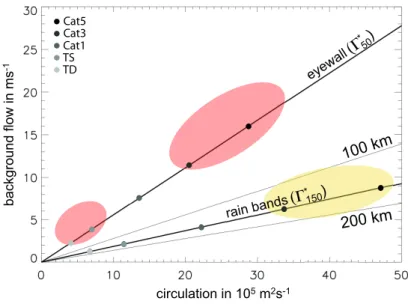
We first note that Eq. (17) provides theoretical support for the hypothesis in RMN that the “character” of shear-TC interaction scales with the ratio of TC intensity and shear magnitude. Here, the shear magnitude is represented by the storm-relative environmental flowU, as discussed in the in-troduction.
The storm-relative environmental flow that is necessary to move the dividing streamline to a specified radiusRnd
in-creases linearly withŴ. For the range of values ofŴ rep-resenting TC intensities from TD to Cat5, we find distinct scenarios of potential environmental interaction (Fig. 8). Di-rect eyewall interaction seems likely for the TD and TS vortices for storm-relative flow starting at approx. 3 ms−1, while storm-relative environmental flow well above 10 ms−1 is necessary to move the dividing streamline to a radius of 50 km for the Cat3 and Cat5 vortices. Estimating that the low-level storm-relative environmental flow is approximately half of the wind difference between 850 hPa and 200 hPa, i.e. the deep-layer vertical “shear”, it can be concluded that direct interaction of environmental air with the eyewall of TCs of tropical storm intensity and below is likely in weak to moderate deep-layer “shear” of 6 ms−1 and above. For mature TCs of category 3 or stronger, a direct interaction of environmental air with the eyewall is unlikely even in strong deep-layer “shear” of 20 ms−1. Note that we have usedŴ50
to derive this result. Due to the slower radial decay of the tan-gential winds in real TCs, these estimates are a lower bound of the required storm-relative flow. Using larger circulation values to represent the respective TC category, e.g.Ŵ150, the
differences between the weak and the strong TC categories are even more pronounced (not shown). For mature storms (category 3 and above), moderate to strong deep-layer shear is likely to promote pronounced interaction of environmental air with rain bands. Such interaction can produce persistent, vortex-scale downdrafts leading to a considerable weakening of the storm (Fig. 5 and RMN).
4.2 An improved estimate of environmental interaction: inward flow rate of environmental air
It is important to note that environmental air can residewithin the dividing streamline also (e.g. Fig. 4a). Potential interac-tion with this environmental air is not accounted for by the estimate presented in the previous subsection. In our sim-ple point vortex framework, environmental air resides within the dividing streamline when the stagnation radius is beyond 250 km. For the Cat1 vortex,rsp>250 km forU <8.9 ms−1
(Eq. 13). Furthermore, the effect of weak convergence above the inflow layer has not been taken into account in Sect. 4.1. We propose that the rateFenvby which environmental air
is transported into the rain band or eyewall region provides an improved estimate for potential environmental interaction in our simple model. The volumetric flow rateFthrough an
area bounded by a curveLand unit height F=
Z
L
vndl, (35)
wheredl is a line segment ofL andvn is the flow normal
todl. The inflow rate of environmental air, Fenv, is
deter-mined from the streamlines that connect the environmental radius and the rain band and eyewall radius, respectively. Streamlines are calculated that emanate along the environ-mental radiusRenv=250 km with a constant azimuthal
spac-ing1φ=3◦. We select a subsetScof these streamlines that
exhibit radial inflow at Renv and connect to the rain band
(eyewall) radius without orbiting the center. The radial flow at radiusrassociated with theith streamline of this subset is denoted byuSi
c(r). Due to mass conservation and the steadi-ness of the flow,Fenvat the rain band (eyewall) radius equals
the radial inflow rate at the environmental radius associated withSc:
Fenv=X
i uSi
c(Renv)Renv1φ. (36)
We exclude orbiting streamlines from our calculation be-cause air parcels along such paths move inwards very slowly. It seems unreasonable to assume that the flow is approxi-mately steady on this longer time scale. Air parcels that spiral through the rain band region towards the eyewall are likely to interact considerably with rain bands before reach-ing the eyewall. It can be assumed that this interaction moist-ens the environmental air considerably before eyewall inter-action takes place. It is, however, an open question if con-vection outside of the eyewall is indeed vigorous enough to protect the inner core from such slow approach of environ-mental air.
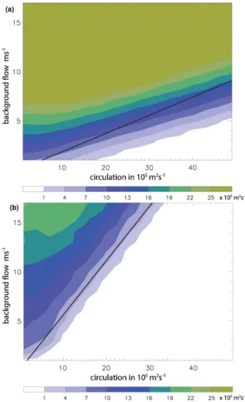
The values ofFenv, calculated from the point vortex with
centered mass sink, are depicted in Fig. 9 for a large part of the phase space relevant for TCs. For comparison, the values ofU andŴfor which the closest approach of the dividing streamlines is at the rain band and eyewall radius, respec-tively, are indicated also. The dividing streamline apparently
gives a good estimate for the onset of potential environmen-tal interaction. In general, low values ofFenv are found for
values ofŴandU for which the dividing streamline is out-side of the rainband (Fig. 9a) and eyewall radius (Fig. 9b), respectively. It is clear thatFenv increases with increasing
U for a given circulationŴ. For eyewall interaction, the lo-cation of the dividing streamline denotes the onset of the in-flow of environmental air extremely well (Fig. 9b). For the rain band region (Fig. 9a), potential environmental interac-tion is slightly underestimated for strong vortices. With this small caveat in mind, the phase space diagram of the divid-ing streamline location (Fig. 8) may be used as a first, simple guidance to estimate the propensity of TC-environment in-teraction.
4.3 A well defined source region of environmental air
As noted in Sect. 2.3 in the discussion of Fig. 6, the source region of environmental air interacting with a TC may ex-hibit a pronounced asymmetric, azimuthal wave number 1 structure. For a Cat1 vortex with U=5.1 ms−1 the enve-lope of streamlines that connect the environment to the rain band radius are overlaid on the flow topology in Fig. 10. It is evident that the main source region of the environmental air that is transported into the rain band region is to the north-west of the storm. Westerly storm-relative flow at low levels indicates that such a TC would be in easterly vertical wind shear.
Now consider a region of very dry air to the southeast of the storm (shaded region in Fig. 10). Although some of this air is located within 200 km of the TC center, the interaction of the dry air with the TC is greatly limited in the easterly wind shear scenario depicted in Fig. 10: the dry air is located outside of the stable manifold. If the vertical wind shear were westerly, however, the low-level storm-relative flow would be from the east. The pattern of the flow topology would be rotated by 180◦and would indicate a pronounced intrusion of
the very unfavorable dry air masses into the TC circulation. This brief discussion demonstrates that in the presence of moisture gradients the adverse impact of vertical wind shear on a TC may be sensitive to the direction of the shear. If the flow topology favors the interaction with particularly dry air masses, a more pronounced weakening of the TC can be expected as in comparison to a shear direction that favors interaction with relatively moist environmental air.
circulation in 105 m2s-1
b
a
ckg
ro
u
n
d
f
lo
w
i
n
ms
-1
eyewa ll
rain bands
200 km
100 km
*
50)
* 150) (Γ
(Γ Cat5
Cat3 Cat1 TS TD
Fig. 8. Regime diagram for the environmental interaction of TCs in vertical wind shear. The sloping lines denote the closest radius of the dividing streamline for a combination of circulation (abscissa) and storm-relative flow (ordinate). For eyewall interaction the TC categories are defined byŴ50, for rain band interactionŴ150is used (see Sect. 3.2.1). The TC categories are highlighted by the shaded dots. The red
shading indicates the regime of eyewall interaction for weak and mature TCs (as defined in Table 1), respectively. Yellow shading indicates the regime of rain band interaction for mature TCs. The eyewall radius (50 km), 100 km radius, the rain band radius (150 km), and 200 km radius are depicted (from top to bottom).
less susceptible to easterly than to westerly environmental shear. Future work should test both hypotheses for the poten-tial importance of the shear direction for TC intensity change, e.g. in an idealized modeling framework.
5 Conclusions
The flow topology of a numerically simulated, idealized TC in vertical wind shear has been examined under the assump-tion of steady and layer-wise horizontal flow. Our results show that for an intense TC, the stagnation point and the as-sociated manifolds are found at significantly larger radii than previously hypothesized (WMF84). The layer-wise horizon-tal flow is weakly convergent above the layer of strong in-flow associated with surface friction and below the outin-flow layer, i.e. approx. between 1.5 km–10 km height. The unsta-ble manifold spirals inwards and ends in the limit cycle, a dividing streamline that encompasses the eyewall in our ide-alized experiment at all levels. From the perspective of the steady and layer-wise horizontal flow model, the eyewall is well protected from the intrusion of environmental air. Time-dependent and/or vertical motions, which are prevalent in the TC inner-core, are necessary to allow intrusion of environ-mental air into the inner-core convection.
The TC’s moist envelope, high-θe air that surrounds the eyewall in the inner core, is strongly distorted by the storm-relative environmental flow. At 2 km height, the moist
enve-lope is highly asymmetric with very lowθeair within 100 km of the center in the downshear-left quadrant of the storm. In the downshear-right quadrant, high-θeair extends to 150 km radius at this height. The shape of the moist envelope is closely related to the location and shape of the limit cycle, with the highestθe air being contained within the limit cy-cle. We conclude that the distribution of high- and low-θe around the TC at low to mid-levels (approx. between 1.5 km and 5 km) is governed in the first approximation by the stir-ring of convectively modified air by the steady, horizontal flow.
Strong and persistent downdrafts occur where precipita-tion from the helical updrafts within the staprecipita-tionary band com-plex falls into relatively dry, low-level environmental air out-side of the limit cycle. The steady supply of dry environmen-tal air in this region promotes the persistence and amplitude of the downdraft pattern. In the first 12 h following the im-position of vertical shear, air from the north and west of the center (downshear and downshear right) feeds into the down-draft region. Subsequently, the downdown-draft region is fed also by air that wraps around the center from the east and south. Interaction with air from the east and the south, however, is limited to a small radius (O(200 km)). This radius is even
smaller than indicated by the location of the stable manifold atO(300 km). The source region of the downdraft air clearly
Fig. 9. Inflow rate of environmental air,Fenv, (shaded) at the ra-dius of 150 km indicating rain band interaction(a)and at 50 km indicating eyewall interaction(b)as a function of circulationŴ (ab-scissa) and storm-relative environmental flowU (ordinate). Val-ues are calculated for the point vortex with centered mass sink (D= −1.5×10⁵m2s−1). The solid line denotes the values ofŴ
andUfor which the closest distance of the dividing streamline from the center is at the rain band(a)and eyewall(b)radius, respectively (cf. Fig. 8).
presence of a pronounced environmental moisture gradient, vertical wind shear may thus promote or impede the interac-tion with dry environmental air, depending on the direcinterac-tion of the shear vector.
To further understand the flow kinematics, an analogue model based on a weakly convergent point vortex in back-ground flow was developed. This simple kinematic model is demonstrated to capture several salient features of the flow topology in the numerical experiment. Assuming a generic distribution of air masses around the TC in a hypothetical “real-world” application, the potential for environmental
in-Fig. 10. Same as Fig. 7, but for a Cat1 vortex in westerly storm-relative environmental flow ofU=5.1 ms−1. The dashed curves denote the envelope of streamlines for which environmental air reaches the “rain band” region in this scenario. The source region of air that interacts with the TC is indicated to the northwest. The area shaded in blue indicates a hypothetical region of very dry en-vironmental air.
teraction can then be quantified by the inflow rate of environ-mental air to the radius of the principal rain band and eyewall, respectively. The location of the dividing streamline provides a simple, yet adequate approximation for the propensity of environmental interaction. The closest approach of the di-viding streamline to the vortex center is proportional to the ratio of the vortex strength and the storm-relative environ-mental flow. Under the assumption that the low-level storm-relative flow is approximately one half of the difference be-tween the low- and the upper-level flow, distinct scenarios of possible environmental interaction are implicated for the range of point vortices and background flows that represent typical conditions of TCs in vertical wind shear. The results suggest that it is not only the dynamic resiliency of a TC that increases with intensity and vortex size (Jones, 1995; Reasor et al., 2004). The ability of a TC to isolate itself from ad-verse thermodynamic interaction with dry environmental air increases considerably with intensity and size also.
Appendix A
Relative importance ofDandUfor environmental interaction