Abstract
In engineering systems design, theoretical deterministic solutions can be hardly applied directly to real-world scenarios. Basically, this is due to manufacturing limitations and environmental condi-tions under which the real system will operate. Therefore, a small variation in the design variables vector can result in a meaningful change on the theoretical optimal design as represented by the minimization of the corresponding vector of objective functions. In this context, it is important to develop methodologies that are able to produce solutions (even suboptimal) that are less sensitive to perturbations in the design variable vector and, consequently, leading to a robust optimal design. In this contribution, first the proposed approach is tested on various mathematical functions. Then, the methodology is applied to the design of two representa-tive engineering systems through multi-objecrepresenta-tive optimization using the Firefly Colony Algorithm in association with the Effec-tive Mean Concept is presented.The results obtained demonstrate that the design strategy conveyed represents an interesting alter-native approach to obtain robust design for a number of engineer-ing applications.
Keywords
Robust Multi-objective Optimization, Pareto's Curve, Effective Mean, Firefly Colony Algorithm.
Robust Multi-objective Optimization Applied
to Engineering Systems Design
1 INTRODUCTION
Frequently, during engineering system design, the model, the design variable vector, andthe param-eter vector are consideredfree of errors, i.e., they do not contain uncertainties. However, more realis-tically, small variations in the design variable vector can cause significant variations in the vector of
Fernando Ricardo Moreira a Fran Sérgio Lobato b Aldemir Ap. Cavalini Jrc Valder Steffen Jr d
a Department of Mathematics, Federal University of Goiás, BR 364, km 195, 3800, Campus Cidade Universitária, 75801-615, Jataí-GO, Brazil. [email protected]
b School of Chemical Engineering, [email protected]
c,d LMEst-Structural Mechanics Laboratory, School of Mechanical Engineering Federal University of Uberlândia Av. João Naves de Ávila 2121, Campus Santa Mônica, P.O. Box 593, 38408-144, Uberlândia-MG, Brazil. [email protected]
http://dx.doi.org/10.1590/1679-78252801
objective functions. As mentioned by Ritto et al. (2008), the process of modeling engineering sys-tems introduces two types of uncertainties: i) uncertainties related to the parameters of the model, such as geometrical and constitutive parameters (data uncertainties), and ii) uncertainties due to the proposed model. In this case, regarding the existence of uncertainties in real-world engineering systems, some aspects should be highlighted (Leidemer, 2009):
Even if the real optimum is found, it will never be possible to implement it in practice, be-cause there are uncertainties associated to the manufacture process or even due to the de-mand of a high degree of accuracy, which can be extremely difficult to achieve or economical-ly unaffordable;
The formulation of optimization problems is inherently static, but the reality is essentially dynamic. In this context, the design problems can be associated with parameter vector fluc-tuation, such as temperature, wind speed, humidity. There might also be waste of some com-ponents that imply alteration in system behavior.
Consequently, the system to be optimized can be very sensitive to small changesin the design variable vector, and thus, small variations in this vector can cause significant changes in the vector of objective functions (Leidemer, 2009). In this context, it is important to determine a methodology that produces solutions less sensitive to small variations in the design variables vector. Solutions with this characteristic are called robust solutions and the procedure to find these solutions is named Robust Optimization (Taguchi, 1984).
Real-world problems involve the simultaneous optimization of two or more (often conflicting) objectives, known as multi-objective optimization problem (MOOP). The solution of such problems is different from that of a single-objective optimization problem, i.e., multi-objective optimization problems normally have not only one but a set of solutions, which may all be equally good (Deb, 2001).
In the literature, several methods for solving MOOP can be found. These methods follow a preference-based approach, in which a relative preference vector is used to scalarize multiple objec-tives. Since classical searching and optimization methods use a point-by-point approach, through which the solution is successively modified, the outcome of this classical optimization method is a single optimized solution. However, Evolutionary Algorithms (EA) can find multiple optimal solu-tions in one single simulation run due to their population-based search approach. Thus, EA are ideally suited for multi-objective optimization problems. A detailed account of multi-objective opti-mization using EA and applications using genetic algorithms are widely found in the literature (Deb, 2001).
communi-cation among the individuals of the population. Each individual is able to capture the changes in the environment as generated by local interactions (Yang, 2008).
Therefore, in this contribution a systematic methodology to solve robust multi-objective optimi-zation problems is proposed. This optimioptimi-zation strategy is based on the Effective Mean Concept - EMC (DebandGupta, 2006) in association with the Multi-objective Optimization Firefly Colony Algorithm – MOFCA (Lobato et al., 2011). The organization of this article is as follows. Section 2 introduces briefly the EMC, the MOFCA and robust multi-objective optimization. For illustration purposes, section 3 presents applications involving mathematical functions and two engineering case studies. Finally, the conclusions are presented in the last section.
2 MULTI-OBJECTIVE OPTIMIZATION FIREFLY COLONY ALGORITHM
In this section, the mean effective concept and the robust multi-objective optimization problem will be defined. In addition, the subroutine of the MOFCA algorithm will be briefly discussed.
2.1 Robust Multi-Objective Optimization
Traditionally, during the solution of optimization problems it is commonly considered that mathe-matical models, variables, and parameters are sufficiently reliable, i.e., there are no errors of model-ing and estimation (DebandGupta, 2006). However, as previously mentioned, systems to be opti-mized are generally sensitive to small changes in the design variables leading to significant changes in the vector of objective functions. In this case, to minimize this effect in the solution of optimiza-tion problems, the concept of robust optimizaoptimiza-tion should be used. Robust Optimizaoptimiza-tion is defined as an approach that produces a solution that is not significantly sensitive to small changes in the de-sign variables (Taguchi, 1984). In this context, robustness characterizes an important dede-sign level to be achieved, when exposed to a given condition of uncertainty. In addition, this approach is used for modeling optimization problems under uncertainty, where the modeler aims at finding decisions that are optimal for the worst-case realization of the uncertainties within a given set of values (Taguchi, 1984).
The introduction of robustness in the mono and multi-objective contexts requires the considera-tion of new restricconsidera-tions and/or new objectives (relaconsidera-tionshipbetween the mean and the standard deviation of the vector of objective functions) and probability distribution functions for the design variables and/or objectives. As mentioned by Ritto et al. (2008) and also considered by Soize (2005), Paenk et al. (2006), and Sampaio and Soize (2007), probability tools are required to model the uncertainties, i.e., random variables are associated with the uncertain parameters or matrices; then, probability density functions are constructed.
In the present contribution, a robustness measure, which does not use the hypothesis on uncer-tainty parameters,will be used. The robustness measure and the solution of a robust multi-objective optimization problem are defined as (DebandGupta, 2006):
Definition - Being f :W Ì n an integrable function. The EMCof f , in relation to a
neigh-borhood dof variable x, is a function feff( , )x d , given by:
( ) 1
( , ) ( )
( )
eff
y B x
f x f y dy
B x
d d
d
Î
=
ò
(1)wheren is the number of design variables.
Definition - A point x*is defined as robust multi-objective solution if it is a Pareto-optimal
solu-tion for the following multi-objective optimizasolu-tion problem, defined byconsidering the neighborhood
dof the variablex:
1 2
min eff( , ), eff( , ), ... , eff( , ) m
f x f x f x (2)
1
subject to eff( , ) 0, 1,..., ; n
g x j k x (3)
where the symbol B xd( ) indicates the hyper-volume of the neighborhood and m is the number of objectives.
To estimate the integral defined by Equation(1), a sample is created randomly by using the Latin Hypercube method (Viana, 2008). Moreover, this procedure increases the computational cost due to additional objective function evaluations that are necessary to solve the optimization prob-lem (DebandGupta, 2006). The Equations (2) and (3) considersan optimization probprob-lem with m objectives and k inequality constraints.
2.2 Firefly Colony Algorithm
The FCA is based on the interesting characteristics of the fireflies’ bioluminescence. The fireflies are insects notorious for their light emission. Although biology does not have a complete knowledge to determine all the utilities that the firefly luminescence can bring to, at least three functions have been identified (Yang, 2008): i) as a communication tool and appeal to potential partners in the reproduction, ii) as a bait to lure prey for the firefly, iii) as a warning mechanism for potential predators reminding them that fireflies have a bitter taste.
In the FCA, the attractiveness between two fireflies is determined by thelight intensity emitted and by the distance between them. The intensity is a function of the objective function (Yang, 2008). An effective exploration of the design space is obtained by the movement of fireflies accord-ing to the attractiveness of other swarm members with higher intensity of light emitted and a ran-dom step vector to avoid a premature convergence. Thus, at the k-th iteration, the movement of the i-th firefly towards the firefly that is more attractive is defined by the following equation (Yang, 2008):
(
)(
)
( )1 exp 2 1 1 0, 5
t t t t
i i j i
wherer is the distance between two fireflies;w andgare parameters defined as the maximum at-tractiveness (when r=0) and the coefficient of light absorption, respectively. The second factor of the right hand side of Equation (4) adds the attractiveness between the fireflies, and the third one, regulated by k, adds randomness to the process.
2.3 Multi-Objective Optimization Firefly Colony Algorithm
Due to the success obtained by the FCA in different science and engineering applications (Apos-tolopoulos and Vlachos, 2011; Lukasik and Zak, 2009; Yang, 2009; Pfeifer and Lobato, 2010),Lobato et al. (2011) proposed the Multi-objective Optimization Firefly Colony Algorithm (MOFCA). This approach is based on the classical FCA associated with Fast Non-Dominated Sorting and has the following structure:
An initial population with Nfirefly fireflies is randomly generated;
All dominated solutions are removed from the population through the operator Fast Non-Dominated Sorting (Deb et al., 2000). In this way, the population is sorted into non-dominated fronts (sets of vectors that are non-non-dominated with respect to each other);
Then, FCA is applied to generate the new population of fireflies (potential candidates to solve the multi-objective optimization problem);
If the number of individuals of the population is larger than the number early defined by the user, it is truncated according to a criterion named the Crowding Distance (Deb et al., 2000).
These steps are repeated until a given stopping criterion is reached. The operators used in the MOFCA are described below.
Fast Non-Dominated Sorting
Fast Non-Dominated Sorting operator was proposed by Deb et al. (2000) in order to sort a popula-tion of size N according to the level of non-dominapopula-tion. Each solupopula-tion must be compared with every other solution in the population to find if it is dominated. At this point, all individuals in the first non-dominated front are found. In order to find the individuals in the next front, the solutions of the first front are temporarily discounted and the above procedure is repeated. The procedure is repeated to find the subsequent fronts.
Crowding Distance Operator
This operator describes the density of solutions surrounding a vector. In order to compute the Crowding Distance for a set of population members, the vectors are sorted according to their objec-tive function values for each objecobjec-tive function. An infinite Crowding Distance (or an arbitrarily large number for practical purposes) is assigned to the vectors with the smallest or largest values. For all other vectors, the Crowding Distance (distxi ) is calculated according to (Deb et al., 2000):
, 1 , 1
,max ,min 1
i m
i j i j x
i i
j
f f
dist
f f
+
-=
-=
wherefj corresponds to the j-th objective function andmis the number of objectives. This operator is important to avoid many points close in Pareto's Curve and to promote the diversity in terms of the space of objectives (Deb et al, 2000).
Treatment of Constraints
In this work, the treatment of constraints is performed through the Static Penalization Method, proposed by Castro (2001). This approach consists in assigning limit values to each objective to play the role of penalization parameters. According to Castro (2001), it is guaranteed that any non-dominated solution dominate any solution that violates at least one of the constraints. In the same way, any solution that violates only one constraint will dominate any solution that presents two constraint violations, and so on. For a constrained problem the vector containing the objective functions to be accounted for, is given by:
( ) ( ) p viol
f x º f x +r n (6)
wheref x( ) is the vector of objective functions, rp is the vector of penalty parameters that depends
on the type of problem considered, and nviol is the number of violated constraints. More details
about this optimization strategy can be found in Lobato et al. (2011).
In the present paper, the methodology proposed by Deband Gupta (2006) considering the EM-Cis used to insert robustness in the MOFCA. In this case, the original objective function vector is transformed by considering Eq. (2). In addition, to evaluate Eq. (1) the Latin Hypercube method is used. It is important to observe that in real-world engineering problems, it is not possible to per-form the analytical calculation of effective mean. Thus, the integration is perper-formed numerically using the Trapezoidal Method.
The user has to inform to the routine the vector of objective functions, the vector of constraints, the design space, the MOFCA parameters, the perturbation di added to the design variable vector,
and the sample size Nsample. To compute the Effective Mean, the user has to inform the value of di
for each design variablexi, which will be calculated by the Latin Hypercube Method.
3 APPLICATIONS
For illustration purposes, in this section, applications involving mathematical functions and the design of two representative engineering systems (the optimum design of an industrial robot and the optimization of a flexible rotor)are presented.
The MOFCA parameters considered for all the applicationsare the following (Lobato et al., 2011):
Fireflies number (Nfirefly) = 55;
Generation number (Ngen) = 250;
Absorption (w)and attractiveness coefficients (g)=1;
Considering the parameters presented above, Nfirefly+Nfirefly Ngenobjective function evaluations are necessary to solve the nominal cases by using the MOFCA. In order to solve the robust cases by the MOFCA, Nfirefly+Nfirefly Ngen Nsampleobjective function evaluations are necessary.
Regarding the mathematical problems, ten simulations for different initial seeds of the random number generator rand aretaken into account to evaluate the convergence and diversity of the solu-tions obtained by using the MOFCA. To compute the convergence metric (CM ) and diversity met-ric (DM)for the cases tests where the analytic solution is known, the following equations are used (Deb, 2001): = i firefly d CM N
å
(7)(
)
= 1f l i m
f l firefly m
d d d d
DM
d d N d
+ +
-+ +
å
- (8)wheredi is the smaller Euclidean distance between the firefly xi and the analytic Pareto's Curve,
f
d and dl represents the Euclidean distance between the extreme solutions of the analytic Pareto's
Curve and the non-dominated solutions obtained through the MOFCA, and dm is the arithmetic
average of di.In this case, the analytic Pareto's Curve was obtained by using 1000 points equally
spaced in order to compute CMand DM.
3.1 Mathematical Problem MP1
The mathematical problem MP1 is defined by (DebandGupta, 2006):
1 1 5 1
5 2
2 1 5 2 1
3 ( ,..., )
min
( ,..., ) ( ) 1 50 i
i
f x x x
f x x h x x x
=
ì =
ïï
ïï æ ö
í ç ÷
ï = ç - + ÷
ï ç ÷
ï çè ÷ø
ïî
å
(9)
where
( )
(
2)
2(
2)
22
0.35 0.85
2 0.8 exp exp
0.25 0.03
x x
h x =ççæç - æççç- - ÷÷ö÷÷- çæçç- - ÷÷÷÷÷÷÷÷öö
è è ø è øø (10)
and 0£x x1, 2 £1 and - £1 xi £1, for i=3, 4 and 5.
ThePareto global and local curves correspond to xi=0 (i=3, 4 and 5) and are obtained from the
global minimum and local minimum of h x( 2), respectively. According toDeb and Gupta (2006), the global and local curves are given by:
2 1 1 (Global)
f = - f (11)
2 1.2(1 1) (Local)
The objectives obtained through the calculation of the EMC are given by the following expres-sions:
1 1eff
f =x (13)
( ) ( )
(
1,5 1,5)
2
1 1
2
3
50 1
1
3 3
n eff
i i i
i i
f d x d x d
d
=
æ æ ö÷ö
ç ç ÷
= Qççè
å
+çèç - + - - ÷ø÷ø÷÷÷ (14)where
(
)
(
)
2 2
2 2
2 2
2
1 0.35 0.85
2 0.8 exp exp
2 0.25 0.03
x
x
y y
dy
d
d d
+
-æ æ - ö÷ æ - öö÷÷
ç ç ç
Q =
ò
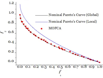
èçç - èçç- ø÷÷÷- ççè- ÷÷÷÷÷÷øø (15)Figure 1 presents the nominal Pareto's Curve (global and local), i.e., without robustness,and the solutions obtained by using MOFCA considering the problem MP1.Note that MOFCA was able to find the global Pareto’s Curve.
Figure 1: Nominal Pareto's Curves (global e local) and the solution obtained by MOFCAfor the problem MP1.
Table 1 presents the metrics computed in each run for the problem MP1. Note thatthe MOFCA converges to the global optimum, except for the run with initial seed equal to zero. In addition, the solutions found by using MOFCA are well distributedon the Pareto's Curve, i.e., there is a good diversity of solutions.
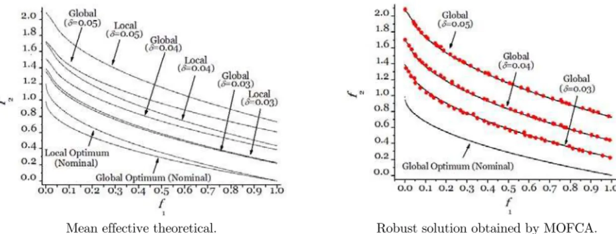
In order to evaluatethe effect of d on the curve, the following perturbation vector [d1 d2 d3 d4
5
Simulations
Metrics 1 2 3 4 5
CM 0.056 0.009 0.014 0.013 0.021
DM 0.423 0.810 1.117 0.660 1.201
Optimum Local Global Global Global Global
Metrics 6 7 8 9 10
CM 0.007 0.020 0.009 0.015 0.012
DM 0.745 1.190 0.832 1.160 0.970
Optimum Global Global Global Global Global
Table 1: Results of the CM and DM metrics for the problem MP1.
Mean effective theoretical. Robust solution obtained by MOFCA.
Figure 2: Influence of parameter don the robust Pareto's Curves for the problemMP1.
In Table 2 it is possible to observe that MOFCA converges to the global optimum for all the simulations performed.
3.2 Mathematical Problem MP2
Mathematically, the problem MP2 can be formulated as follows (Deband Gupta, 2006):
( 1 2 ) ( 1 1 1 )
min f x( ), ( )f x = x h x, ( )+G x S x( ) ( ) (16)
subject to
1 2
( ) 0.2 0.1 0
g x = x +x - ³ (17)
where
2
1 1
( ) 1
h x = -x (18)
5 2
2
( ) 50 i
i
G x x
=
2
1 1
1 1 ( )
0.2
S x x
x
= +
+ (20)
and 0£x1 £1 and - £1 xi £1, for i=2, 3, 4 and 5.
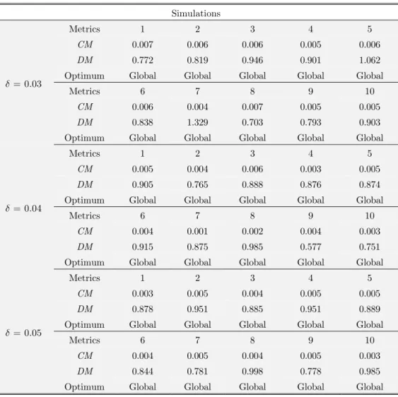
Simulations
0.03
d =
Metrics 1 2 3 4 5
CM 0.007 0.006 0.006 0.005 0.006
DM 0.772 0.819 0.946 0.901 1.062
Optimum Global Global Global Global Global
Metrics 6 7 8 9 10
CM 0.006 0.004 0.007 0.005 0.005
DM 0.838 1.329 0.703 0.793 0.903
Optimum Global Global Global Global Global
0.04
d =
Metrics 1 2 3 4 5
CM 0.005 0.004 0.006 0.003 0.005
DM 0.905 0.765 0.888 0.876 0.874
Optimum Global Global Global Global Global
Metrics 6 7 8 9 10
CM 0.004 0.001 0.002 0.004 0.003
DM 0.915 0.875 0.985 0.577 0.751
Optimum Global Global Global Global Global
0.05
d =
Metrics 1 2 3 4 5
CM 0.003 0.005 0.004 0.005 0.005
DM 0.878 0.951 0.885 0.951 0.889
Optimum Global Global Global Global Global
Metrics 6 7 8 9 10
CM 0.004 0.005 0.004 0.005 0.003
DM 0.844 0.781 0.998 0.778 0.985
Optimum Global Global Global Global Global
Table 2: Results of the CM and DM metrics obtained for the robust problem MP1.
In this problem, the nominal Pareto's Curve is obtained by the activation of the constraint equations, i.e., when x2 =0.1-0.2x1 and considering xi=0 for i=2, 3, 4 and 5. As observed in the
previous case, the objectives obtained by EMC are expressed by:
1 1 ( , )
eff
f x d =x (21)
2
1 1
2
1 2 1
1 se 0, 5
se 0, 5
eff x x
f
H H x
ì - ³
ïïï = íï
<
ïïî (22)
(
)
5 21 1 1
2 2 2 2
1 1 1 1
1 1 1 3
1 0.2 1 100
1 log
3 2 0.2 3 i 3 i
x
H x x
x
d d d d
d d =
æ æ + + ö÷ ö÷
ç ç
= - - +èçç èçç ÷÷ø+ + ÷÷ø
+ -
å
(23)( )
1 1
1 1
2 2
2 1 2
1
50 1
0.1 0.2 0.2
2 0.2
x
x
H y y dy
y
d
d
d d d
+
-æ ö÷
ç
= ççè + ÷÷ - + +
ø +
ò
(24)Table 3 presents the CM and DM metrics for the nominalproblemMP2.
Simulations
Metrics 1 2 3 4 5
CM 0.025 0.031 0.019 0.021 0.019
DM 0.974 1.063 0.655 0.625 0.484
Metrics 6 7 8 9 10
CM 0.025 0.022 0.037 0.025 0.016
DM 0.974 0.723 1.077 0.911 0.672
Table 3: Results of the CM and DMmetrics for the problem MP2.
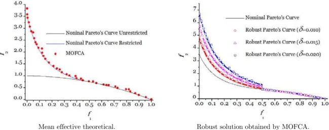
Figure 3(a) presents the nominal Pareto's Curve without and with the constraint and the solu-tion obtained by using the MOFCA. It is possible to observe that satisfactory resultsare obtained for both convergence and diversity.
Mean effective theoretical. Robust solution obtained by MOFCA.
Figure 3: Nominal Pareto's Curve obtained by MOFCA for the problem MP2 considering rp equal to 106.
To evaluate the effect ofdon the Pareto's Curve, a perturbation vector [d1 d2 d3 d4 d5] = [d 2d
2d 2d 2d] was considered. In this case, d=[0.0100.0150.020]. In Figure3(b) the results obtained by using MOFCA considering different values ofd are shown. For each run, a good distribution of the solutions on the Pareto's Curve is observed. As mentioned by Deb and Gupta (2006), the analytical Pareto's Curve can be described by two regions defined for x1, which is smaller than 0.5. On the
other hand, considering x1greater than 0.5, the constraint is always attended, independently of the
Table 4 presents the CMand DM metrics for different values of d. It is possible to observe that the obtained values for the metrics are satisfactory, i.e., the CM tends to small values and the
DMmetric values present good distribution (see Figure 3(b)).
Simulations
δ .010
Metrics 1 2 3 4 5
CM 0.161 0.120 0.162 0.067 0.039
DM 1.372 1.366 1.451 1.098 0.706
Metrics 6 7 8 9 10
CM 0.080 0.092 0.043 0.056 0.167
DM 1.057 1.195 0.779 1.034 1.429
δ 0.015
Metrics 1 2 3 4 5
CM 0.145 0.115 0.143 0.044 0.045
DM 1.309 1.278 1.409 1.024 0.678
Metrics 6 7 8 9 10
CM 0.079 0.078 0.040 0.045 0.179
DM 1.087 1.012 0.756 1.033 1.409
δ 0.020
Metrics 1 2 3 4 5
CM 0.114 0.105 0.124 0.056 0.030
DM 1.955 1.232 1.533 1.087 0.712
Metrics 6 7 8 9 10
CM 0.090 0.089 0.043 0.070 0.145
DM 1.067 1.342 0.766 1.033 1.389
Table 4: Results of the CM and DM metrics obtained for the robust problemMP2.
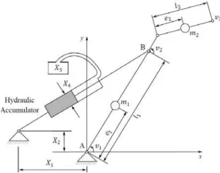
3.3 Industrial Robot
This real-world engineering application was first proposed by Eschenauer et al. (1990) and considers the optimization of an industrial robot, in which a hydraulic spring mechanism is used for the bal-ancing of the armAB (see Figure 4).
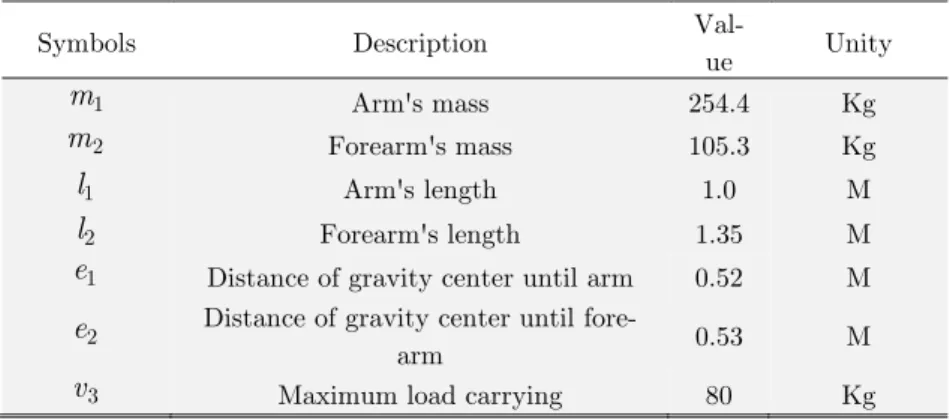
Table 5 presents the robot parameters considered in this application.
Symbols Description
Val-ue Unity
1
m Arm's mass 254.4 Kg
2
m Forearm's mass 105.3 Kg
1
l Arm's length 1.0 M
2
l Forearm's length 1.35 M
1
e Distance of gravity center until arm 0.52 M
2
e Distance of gravity center until
fore-arm 0.53 M
3
v Maximum load carrying 80 Kg
Table 5: Industrial robot parameters (Eschenauer et al., 1990).
The design variables associated with the balancing of the robot's arm are the following: localiza-tion of spring mechanism in relalocaliza-tion to base (X1andX2, in meters), pressure of hydraulic
accumu-lator (X3, in MPa), and cylinder diameter (X4, in meters). The robot's performance is a function
of the static torque in steering the motor shaft, the work executed by the motor, and the static force in the joint A. The model of the industrial robot presented in Fig. 1 was obtainedbyupdat-ingof following meta-model:
2 2
0 1 1 4 4 5 1 8 4 9 1 2 10 1 3
11 1 4 12 2 3 13 2 4 14 3 4
... ...
Y x x x x x x x x
x x x x x x x x
b b b b b b b
b b b b
= + + + + + + + + + +
+ + + + (25)
where bi are the approximation coefficients (i = 1, …, 14), xi (i = 1, …, 4) are the design
varia-bles vector, and Y =[y1met y2met y3met] is the vector of response of the model, representing measures
to evaluate the performance of the industrial robot. For this purpose, the design vector variables were coded as (Eschenauer et al., 1990):
1 2 3 4
1 2 3 4
0.3 3.3 0.037
, , ,
0.01 0.04 0.3 0.003
X X X X
x = x = - x = - x = - (26)
According to Eschenauer et al. (1990), a satisfactory performance of the robot depends on the following criteria: static torque on the shaft of the driving motor (y1), work performed by the
driv-ing motor (y2), and the static force at the joint A (y3).
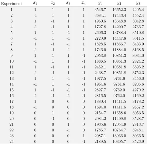
Table 6 presents the experiments considered by Eschenauer et al. (1990), which are now used in this application.
Experiment x1 x2 x3 x4 y1 y2 y3
1 1 1 1 1 3546.7 16652.3 4405.4
2 -1 1 1 1 3684.1 17443.4 4552.4
3 1 -1 1 1 1960.5 13648.9 3042.8
4 -1 -1 1 1 1727.8 14200.7 2736.7
5 1 1 -1 1 2606.3 13788.4 3510.8
6 -1 1 -1 1 2720.9 14447.8 3611.5
7 1 -1 -1 1 1828.5 11856.7 3433.9
8 -1 -1 -1 1 1746.0 11884.0 3168.5
9 1 1 1 -1 2053.8 10851.3 3034.0
10 -1 1 1 -1 1886.5 10851.3 2824.2
11 1 -1 1 -1 2452.1 10581.8 3895.2
12 -1 -1 1 -1 2438.7 10851.8 3752.3
13 1 1 -1 -1 1977.5 9761.6 3456.0
14 -1 1 -1 -1 1954.6 9761.6 3205.6
15 1 -1 -1 -1 2827.7 9762.0 4270.2
16 -1 -1 -1 -1 2816.5 9762.0 4169.2
17 1 0 0 0 1880.4 11411.5 3178.2
18 -1 0 0 0 1694.0 11411.5 2857.2
19 0 1 0 0 2154.7 11658.6 3053.5
20 0 -1 0 0 2084.2 11409.8 3528.7
21 0 0 1 0 1935.6 12054.9 2813.7
22 0 0 -1 0 1785.7 10764.7 3248.1
23 0 0 0 1 2087.1 13966.0 3066.5
24 0 0 0 -1 2189.5 10305.7 3526.9
Table 6: Experimental data planning and answer obtained for the industrial robot application (Eschenauer, 1990).
Coefficient y1met y2met y3met
0
b 1838.77 11416.08 3023.20
1
b 25.80 -127.75 74.93
2
b 150.17 626.97 -19.11
3
b 79.00 852.64 -56.50
4
b 72.83 1966.61 -33.61
5
b -51.57 -4.58 -5.50
6
b 280.67 131.61 267.89
7
b 21.87 -6.28 7.69
8
b 299.52 719.76 273.49
9
b -25.10 -37.58 -37.68
10
b 17.12 -57.88 -0.26
11
b -9.47 -109.97 -23.76
12
b 159.46 126.27 165.43
13
b 497.36 654.58 454.08
14
b 172.66 367.46 162.99
2
Table 7: Meta-model coefficients and determination coefficient (R2) for the industrial robot application.
Robust Optimum Design
The formulation for the multi-objective optimization problem is given by (Eschenauer et al., 1990):
1 1 2 3 4 1
2 1 2 3 4 2
3 1 2 3 4 3
( , , , )
min ( , , , )
( , , , )
met
met
met
f x x x x y
f x x x x y
f x x x x y
ìï =
ïï
ïï =
íï
ïï =
ïïî
(27)
where - £1 xi £1, i = 1, 2 , 3 and 4.
The following relation [d1 d2 d3 d4] = [d d d d] was considered to evaluate the robustness of
the design, in which dis equal to 0.1 and 0.2. These values represent a disturbance of 5% and 10%, respectively, in the amplitude of the domain of definition of the design variables.
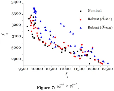
Figures 5 to 7 present the vector of objective functions, where the comparison between the nom-inal and robust cases for d equal to 0.1 and 0.2 is performed.
Figure 5: y1met´y2met.
Figure 7: y2met´y3met.
It can be observed that for the solutions in the interval 9500 £f2 £ 10000 there is a high
sensi-tivity of the objectives f1and f3, thus characterizing a zone of small robustness. On the other hand,
from the identification of regions with small robustness, it is also possible to identify zones with low sensitivity of the objectives, i.e., the robustness zones.
3.4 Flexible Rotor
Rotating machines are used in a wide range of applications regarding different engineering fields, such as automotive, aerospace and power generation industries. The generator units of hydraulic power plants, jet engines, steam turbines, are some examples of applications (Tsuzuki, 2012; Cava-lini Jr, 2013). Therefore, the identification of optimal design and operating conditions for such kind of machines is an interesting engineering challenge (Quitzrau, 2002). Assis(1999) applied optimiza-tion techniques to identify unknown parameters of a vertical rotating machine. A similar procedure was adopted by Steffen Jr et al. (1999) by using multi-objective optimization techniques. He et al. (2001) applied the Genetic Algorithm associated to a finite element model to detect cracks in a rotating shaft. Bueno (2007) used optimization techniques to obtain the optimal localization of pie-zoelectric sensors and actuators for active vibration control. Cavalini Jr(2013) identified incipient cracks in a rotating shaft by using a nonlinear phenomenon and the Differential Evolution Algo-rithm.
Robust Optimum Design
flexible steel shaft with 552 mm length and 12 mm of diameter (nominal diameter;
E
= 210 GPa,r
= 7800 kg/m3, u= 0.3), three rigid discs of steel (see Table 8;r
= 7800 kg/m3), and two identi-cal ball bearings (m = 10 kg,k
xx=
k
zz= 106 N/m,k
xz=
k
zx=0,c
xx=
c
zz=83.3 N/m andxz zx
c
=
c
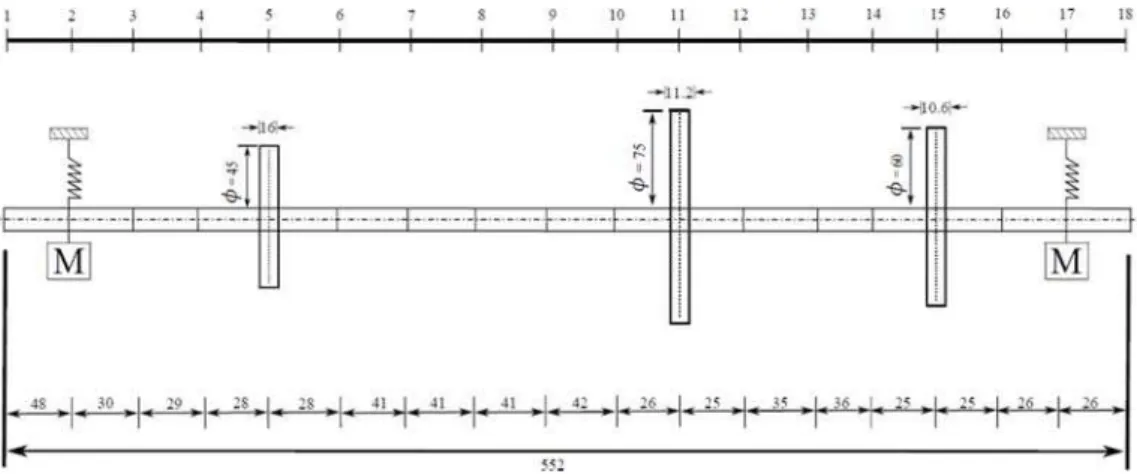
= 0). Considering the nominal parameters, the first two forward critical speeds of the rotor are approximately: 2620 rev/min and 2940 rev/min.Figure 8: Finite element model for the studied rotor.
Table 8 presents the geometric characteristics of the discs of the rotor.
Disc Mass (kg) Moment of Inertia (kg m2) Radius
(mm) Depth (mm)
1 0.794 0.005 45 16
2 1.544 0.005 75 11.2
3 0.935 0.005 60 10.6
Table 8: Geometric characteristics of the discs of the rotating machine.
The robust optimization process was formulated to deal with 4 design variables, namely the ex-ternal radius of the finite elements confined between nodes 1 to 5; 5 to 11; 11 to 15 and 15 to 18 (see Fig.8). Table 9 shows the design space used in the fitting of the finite element model. In order to avoid assembly problems, the external radius of the shaft associated with the nodes 5 to 11 is given by the sum of the radius determined for the first shaft section (nodes 1 to 5) and the ones for the second section (nodes 5 to 11). Similar procedure was adopted for the sections associated with nodes 11 to 15 and 15 to 18.
Shaft section (nodes) Lower limit (m) Upper limit (m)
to 5 0.004 0.008
5 to 11 0 0.004
11 to 15 0 0.004
15 to 18 0.004 0.008
The robustness evaluation of the solution was performed considering the deviation parameters 1
d
= 0.0005 m,d
2= 0.00075 m andd
3= 0.001 m, separately, which represent perturbations of 8.33%, 12.5%, and 16.67%, respectively, on the nominal radius of the shaft.Figure 9 shows the deterministic and robust Pareto's Curve obtained by using the MOFCA al-gorithm. In this case, both objectives are sensible to small perturbations on the design variables. The first critical speed presents a variation of 2000 rev/min approximately, while the third one reaches 4800 rev/min (nominal value of 2940 rev/min). The robust region for the optimum design of the rotating machine is verified. Note that the third critical speed increases according to
d
(per-turbation parameter) for the case in which a single first critical speed is considered.Figure 9: Deterministic and robust Pareto's Curve obtained by using the MOFCA algorithm.
Table 10 presents the optimal solutions determined from the deterministic and robust process considering the highly fireflies of Figure 9.
Shaft section (nodes) Deterministic (m) r1 (m) r2 (m) r3 (m)
to 5 7.76 10-3 6.01 10-3 6.10 10-3 7.89 10-3
5 to 11 3.73 10-3 3.47 10-3 4.05 10-5 2.67 10-4
11 to 15 5.67 10-4 4.03 10-4 5.34 10-4 4.20 10-4
15 to 18 5.27 10-3 4.90 10-4 5.62 10-3 4.60 10-3
3 1
Cr -Cr (rev/min) 1197.7 1214.4 1206.2 1306.6
Table 10: Optimal solutions determined from the deterministic and robust process (Criis the critical speed).
Figures 10 and 11 shows the Campbell diagrams obtained from the nominal radius of the shaft and the one obtained at the end of the optimization process considering the robust (r2) solution,
Figure 10: Campbell diagram for the nominal case.
Figure 11: Campbell diagram for the robust (r2) case presented in Table 10.
4 CONCLUSIONS
In this contribution, the Multi-objective Optimization Firefly Colony Algorithm in association with the Effective Mean Concept was used to solve robust multi-objective problems. This methodology was applied to solve both mathematical and real-world engineering problems. In general, for the test cases considered, the results obtained were considered satisfactory as compared with those described in the literature.
In the industrial robot's arm optimization problem, the influence of the robustness parameter d on the robust Pareto's Curve was observed. It was also possible to characterize regions with higher sensitivity of the objectives with respect to small perturbations in the design variables. In the
con-0 1000 2000 3000 4000 5000
30 40 50 60
Rotation speed (rev/ min)
Fr
eq
ue
nc
y
(H
z)
0 1000 2000 3000 4000 5000
30 40 50 60
Rotation speed (rev/ min)
Fr
eq
ue
nc
y
(H
text of robust design, this characterization is of great importance, since regions with greater sensi-tivity have to be crowded out in relation to those with lower sensisensi-tivity.
Considering the results obtained, it is important to mention that the robustness parameter in-fluences the robust Pareto's Curve.
Since a systematic study introducing robustness in multi-objective optimization problems (DebandGupta, 2006; Paenk et al., 2006) is not easily available, the problems studied may serve as comparison for future evaluations of other methodologies for robust multi-objective optimization. Regarding optimal robust design, the determination of robustness regions may represent a criterion for the choice of a specific point of the Pareto's Curve for a possible practical implementation. How-ever, it is important to observe that the main disadvantage of this approach is the increase of the number of objective function evaluations, which are necessary to evaluate the integral considered in the Effective Mean Concept, independently from the optimization strategy considered.
It is worth mentioning that the operators used in the MOFCA algorithm were not developed in this paper. In addition, the authors of the present contribution did not propose the Mean Effective Concept originally. However, the use of Mean Effective Concept associated to Firefly Colony Algo-rithm represents a new approach, considering the literature associated with this work. The devel-opment of a multi-objective algorithm for the robust optimization using the FCA is considered as being the main contribution of the present contribution.
Further works will be dedicated to approaches related to dynamically updating the parameters and mutation strategies of the Multi-objective Optimization Firefly Colony Algorithmtogether with its parallelization to reduce the number of objective function evaluations.
5 ACKNOWLEDGEMENTS
The authors are thankful to the Brazilian research agencies CNPq, FAPEMIG and CAPES for the financial support of this research work through the INCT-EIE.
References
Apostolopoulos T., Vlachos A. (2011). Application of the Firefly Algorithm for Solving the Economic Emissions Load Dispatch Problem. International Journal of Combinatorics 2011, 1–23.
Assis E. G. (1999). Use of Optimization Techniques to Assist the Project and Identify Parameters in Rotating Ma-chines. PHD Thesis (in portuguese), Faculty of Mechanical Engineering, Federal University of Uberlandia – Brazil. Bueno D. D. (2007). Active Control of Vibrations and Optimal Location of Sensors and Actuators Piezoelectric. Master’s Thesis (in portuguese), Faculty of Engineering of IlhaSolteira, State University Paulista.
Castro R. E. (2001). Structural Optimization with Multiobjectives through Genetic Algorithms. PHD Thesis (in portuguese), Faculty of Civil Engineering, COPPE/UFRJ – Brazil.
Cavalini Jr. A. A. (2013). Detection and Identification of Cracks Transversal Incipient Axes Flexible Horizontal Rotating Machines. PHD Thesis (in portuguese), Faculty of Mechanical Engineering, Federal University of Uber-landia – Brazil.
Deb K. (2001). Multi-Objective Optimization Using Evolutionary Algorithms. John Wiley & Sons, Chichester, UK, ISBN 0-471-87339-X.
Deb K., Gupta H. (2006). Introducing Robustness in Multiobjective Optimization. Evolutionary Computation 14 (4), 463–494.
Djamaluddin F., Abdullah S., Ariffin A. K., Nopiah Z. M. (2015) Multi Objective Optimization of Foam-filled Circu-lar Tubes for Quasi-static and Dynamic Responses, Latin American Journal of Solids and Structures 12, 1126–1143. Eschenauer H., Koski J., Osyczka A. (1990). Multicriteria Design Optimization - Procedures and Applications. First Edition. Berlin Heidelberg: Springer-Verlag.
Ghashochi-Bargh H., Sadr M. H. (2014) Vibration Reduction of Composite Plates by Piezoelectric Patches using a Modified Artificial Bee Colony Algorithm, Latin American Journal of Solids and Structures 11, 1846–1863.
He Y., Guo D., Chu F. (2001). Using Genetic Algorithms and Finite Elements Methods to detect Shaft Crack for Rotor-Bearing System. Mathematics and Computers in Simulation 57 (1), 95–108.
Leidemer M.N. (2009). Proposal of Evolutionary Robust Optimization Methodology using the Unscented Transform Applicable to Circuits for RF Circuits/Microwave. Master’s Thesis (in portuguese), University of Brasilia – Brazil. Lobato F. S., Arruda E. B., Cavalini Jr. A. Ap., Steffen Jr. V. (2011). Engineering System Design using Firefly Algo-rithm and Multiobjective Optimization. Proceedings of the ASME 2011 International Design Engineering Technical Conferences & Computers and Information in Engineering Conference IDETC/CIE 2011, Washington DC, USA, August 28-31.
Lobato F. S., Steffen Jr. V. (2014) Fish Swarm Optimization Algorithm Applied to Engineering System Design, Latin American Journal of Solids and Structures 11, 143–156.
Lukasik S., Zak S. (2009). Firefly Algorithm for Continuous Constrained Optimization Task. Springer Berlin Heidel-berg 5796, 97–106.
Paenk I., Branke J., Jin Y. (2006). Efficient Search for Robust Solutions by Means of Evolutionary Algorithms and Fitness Approximation. IEEE Transactions on Evolutionary Computation 10, 405–420.
Pfeifer A. A., Lobato F. S. (2010). Solution of Singular Optimal Control Problems using the Firefly Algorithm. Pro-ceedings of VI Congreso Argentino de IngenieriaQuimica - CAIQ2010.
Quitzrau L. E. (2002). Dynamic Analysis of Turbo Groups Rotors and Hydrogenerators with Method of Transfer Matrices. Master’s Thesis (in portuguese), School of Engineering, Federal University of Rio Grande do Sul – Brazil. Ritto T. G., Sampaio R., Cataldo E. (2008). Timoshenko Beam with Uncertainty on the Boundary Conditions. Journal of the Brazilian Society of Mechanical Science and Engineering XXX (4), 295–303.
Sampaio R., Soize C. (2007). On Measures of Nonlinearity Effects for Uncertain Dynamical Systems Application to a Vibro-Impact System. Journal of Sound and Vibration 303, 659–674.
Soize C. (2005). A Comprehensive Overview of a Non-Parametric Probabilistic Approach of Model Uncertainties for Predictive Models in Structural Dynamics. Journal of Sound and Vibration 288 (3), 623–652.
Steffen Jr. V., Assis E. G., Lepore Neto F. P. (1999). Multicriterion Techniques for the Optimization of Rotors. Nonlinear Dynamics, Chaos, Control and their Applications to Engineering Sciences 2, 236–249.
Taguchi G. (1989). Quality Engineering through Design Optimization. Springer-Verlag US pp. 77–96. Tsuzuki M. S. G. (2012). Simulated Annealing - Single and Multiple Objective Problems. Intech pp. 197–216. Viana F. A. C. (2008). Surrogate Modeling Techniques and Optimization Methods Applied to Design and Identifica-tion Problems. PHD Thesis, Faculty of Mechanical Engineering, Federal University of Uberlandia – Brazil.
Yang X. S. (2009). Firefly Algorithm for Multimodal Optimization. Stochastic Algorithms: Foundations and Appli-cations 5792, 169–178.