ACPD
12, 9125–9159, 2012Volcanic ash clouds
A. L. M. Grant et al.
Title Page
Abstract Introduction
Conclusions References
Tables Figures
◭ ◮
◭ ◮
Back Close
Full Screen / Esc
Printer-friendly Version Interactive Discussion
Discussion
P
a
per
|
Dis
cussion
P
a
per
|
Discussion
P
a
per
|
Discussio
n
P
a
per
|
Atmos. Chem. Phys. Discuss., 12, 9125–9159, 2012 www.atmos-chem-phys-discuss.net/12/9125/2012/ doi:10.5194/acpd-12-9125-2012
© Author(s) 2012. CC Attribution 3.0 License.
Atmospheric Chemistry and Physics Discussions
This discussion paper is/has been under review for the journal Atmospheric Chemistry and Physics (ACP). Please refer to the corresponding final paper in ACP if available.
Horizontal and vertical structure of the
Eyjafjallaj ¨okull ash cloud over the UK: a
comparison of airborne lidar observations
and simulations
A. L. M. Grant1, H. F. Dacre1, D. J. Thomson2, and F. Marenco2
1
Department of Meteorology, University of Reading, UK
2
Met Office, Exeter, UK
Received: 20 February 2012 – Accepted: 23 March 2012 – Published: 10 April 2012 Correspondence to: H. F. Dacre ([email protected])
ACPD
12, 9125–9159, 2012Volcanic ash clouds
A. L. M. Grant et al.
Title Page
Abstract Introduction
Conclusions References
Tables Figures
◭ ◮
◭ ◮
Back Close
Full Screen / Esc
Printer-friendly Version Interactive Discussion
Discussion
P
a
per
|
Dis
cussion
P
a
per
|
Discussion
P
a
per
|
Discussio
n
P
a
per
|
Abstract
During April and May 2010 the ash cloud from the eruption of the Icelandic volcano Ey-jafjallaj ¨okull caused widespread disruption to aviation over northern Europe. Because of the location and impact of the eruption a wealth of observations of the ash cloud were obtained and can be used to assess modelling of the long range transport of
5
ash in the troposphere. The UK’s BAe-146-301 Atmospheric Research Aircraft over-flew the ash cloud on a number of days during May. The aircraft carries a downward looking lidar which detected the ash layer through the backscatter of the laser light. The ash concentrations are estimated from lidar extinction coefficients and in situ mea-surements of the ash particle size distributions. In this study these estimates of the
10
ash concentrations are compared with simulations of the ash cloud made with NAME (Numerical Atmospheric-dispersion Modelling Environment), a general purpose atmo-spheric transport and dispersion model.
The ash layers seen by the lidar were thin, with typical depths of 550–750 m. The vertical structure of the ash cloud simulated by NAME was generally consistent with the
15
observed ash layers. The layers in the simulated ash clouds that could be identified with observed ash layers are about twice the depth of the observed layers. The structure of the simulated ash clouds were sensitive to the profile of ash emissions that was assumed. In terms of horizontal and vertical structure the best results were mainly obtained by assuming that the emission occurred at the top of the eruption plume,
20
consistent with the observed structure of eruption plumes. However, when the height of the eruption plume was variable and the eruption was weak, then assuming that the emission of ash was uniform with height gave better guidance on the horizontal and vertical structure of the ash cloud.
Comparison between the column masses in the simulated and observed ash layers
25
ACPD
12, 9125–9159, 2012Volcanic ash clouds
A. L. M. Grant et al.
Title Page
Abstract Introduction
Conclusions References
Tables Figures
◭ ◮
◭ ◮
Back Close
Full Screen / Esc
Printer-friendly Version Interactive Discussion
Discussion
P
a
per
|
Dis
cussion
P
a
per
|
Discussion
P
a
per
|
Discussio
n
P
a
per
|
1 Introduction
The eruption of the Icelandic volcano Eyjafjallaj ¨okull during April and May 2010 lead to the widespread disruption of air travel throughout Europe due to the hazard posed to aircraft by volcanic ash. At various times during this period parts of European airspace were closed, leading to significant financial losses by airlines and leaving millions of
5
passengers stranded throughout the world.
During the eruption the London Volcanic Ash Advisory Centre (VAAC) issued fore-casts of the location of the ash cloud. These forefore-casts were based on the NAME (Nu-merical Atmospheric-dispersion Modelling Environment) model (Jones et al., 2007) ad-justed in the light of satellite and ground-based observations. NAME is a Lagrangian
10
particle model that uses time varying wind fields to calculate the turbulent trajectories of particles originating at the position of the volcano to determine where the volcanic ash cloud is transported.
A major uncertainty in modelling volcanic ash clouds with volcanic ash transport and dispersion (VATD) models is the specification of the eruption source parameters (ESP).
15
A VATD model needs information on basic parameters such as the height of the erup-tion plume, the mass eruperup-tion rate and the vertical distribuerup-tion of the emitted mass. The sensitivity of predictions of ash dispersal to the emission profile has been investigated by Webley et al. (2009) for the August 1992 eruption of Mount Spurr. Their study found that the areal extent of the simulated ash cloud was sensitive to assumptions about
20
the emission profile, with the best agreement between the simulations and satellite ob-servations of the extent of the ash cloud obtained using emission profiles which have releases at all heights within the eruption column. Webley et al. (2009) concluded that in this case it was necessary to have ash emitted throughout the atmospheric column. Eckhardt et al. (2008) and Kristiansen et al. (2010) describe a data assimilation
ap-25
ACPD
12, 9125–9159, 2012Volcanic ash clouds
A. L. M. Grant et al.
Title Page
Abstract Introduction
Conclusions References
Tables Figures
◭ ◮
◭ ◮
Back Close
Full Screen / Esc
Printer-friendly Version Interactive Discussion
Discussion
P
a
per
|
Dis
cussion
P
a
per
|
Discussion
P
a
per
|
Discussio
n
P
a
per
|
ash, using SEVIRI (Spinning Enhanced Visible Infra-Red Imager) data for the Eyjafjal-laj ¨okull eruption. In the absence of observational constraints on ESPs, which is likely to be the case during the initial phase of an eruption, Mastin et al. (2009) suggest realistic ESPs for a variety of eruption types that can be used with a VATD model.
The ash cloud from Eyjafjallaj ¨okull over Europe was well observed by ground based
5
lidar (Ansmann et al., 2010) and ceilometers (Flentje et al., 2010). In addition special flights were carried out by the DLR Falcon (Schumann et al., 2011) and the FAAM (Fa-cility for Airborne Measurements) BAE-146 aircraft (Johnson et al., 2011) to provide verification of the ash forecasts. These aircraft were equipped with both in situ particle measuring probes and downward looking lidar. The data collected during the eruption
10
of Eyjafjallaj ¨okull provide an opportunity to evaluate the ash distributions from VATD models in both the horizontal and vertical and the sensitivity of the simulated ash cloud to assumptions about ESPs. In this study the vertically resolved structure of the ash cloud simulated by NAME is compared with lidar data obtained by the FAAM aircraft during May. The comparison is both qualitative, considering the relationship between
15
simulated and observed ash layers, and quantitative, comparing estimates of ash con-centrations from the NAME simulations with estimates obtained from the lidar. The sensitivity of the NAME simulations to assumptions about the profile of ash emissions is also investigated.
2 Model
20
NAME is a Lagrangian particle trajectory model that is designed for use in a range of dispersion modelling applications (Jones et al., 2007). Particles are released at the source, in this case the volcanic eruption plume, with each particle representing a mass of volcanic ash. The trajectories of these particles are calculated here using analysis wind fields from the global version of the Met Office Unified Model, with a resolution of
25
ACPD
12, 9125–9159, 2012Volcanic ash clouds
A. L. M. Grant et al.
Title Page
Abstract Introduction
Conclusions References
Tables Figures
◭ ◮
◭ ◮
Back Close
Full Screen / Esc
Printer-friendly Version Interactive Discussion
Discussion
P
a
per
|
Dis
cussion
P
a
per
|
Discussion
P
a
per
|
Discussio
n
P
a
per
|
parameterisation. NAME also includes treatments of sedimentation and dry and wet deposition (Dacre et al. (2011) for further details). Ash concentrations are computed here by summing the mass of particles in areas of 0.374◦latitude by 0.5625◦longitude,
averaged over 200 m in the vertical and over a time period of 1 h and dividing by volume. Rose et al. (2000) suggested that there are three stages in the evolution of volcanic
5
ash clouds. In the first few hours large particles fallout close to the volcano, forming the proximal tephra blanket. This is followed by a period, typically lasting about 24 h, in which the mass in the ash cloud decreases with time, probably primarily due to particle aggregation and subsequent fallout of the aggregates. During the first two phases a large fraction of the erupted mass is removed from the ash cloud. For the 1992 Mount
10
Spurr eruption only a small fraction of the erupted mass remained in the ash cloud after the first 24 h. Subsequent removal of ash is mainly due to meteorological pro-cesses and deposition. NAME does not represent any of the microphysical propro-cesses, such as aggregation, that occur within the volcanic ash cloud, although it does have representations of particle sedimentation as well as wet and dry deposition.
15
The removal of ash by sedimentation depends on the size distribution of the ash cloud. In situ observations of the ash cloud by the FAAM aircraft over and around the UK show that particles were generally less than 10 µm in diameter (Johnson et al., 2011) in the Eyjafjallaj ¨okull ash cloud. Sedimentation of particles with diameters less than 10 µm has a small effect on column loads for travel times of 24 to 80 h, relevant to
20
this study. This has been determined by testing the sensitivity of the results to different particle sizes (Dacre et al., 2012). Because of this the evolution of the particle size distribution in the ash cloud due to sedimentation has been neglected by setting the particle size to 3 µm. In comparing the lidar observation with NAME a virtual source strength for the fine ash particles which formed the ash layers seen by the lidar can
25
ACPD
12, 9125–9159, 2012Volcanic ash clouds
A. L. M. Grant et al.
Title Page
Abstract Introduction
Conclusions References
Tables Figures
◭ ◮
◭ ◮
Back Close
Full Screen / Esc
Printer-friendly Version Interactive Discussion
Discussion
P
a
per
|
Dis
cussion
P
a
per
|
Discussion
P
a
per
|
Discussio
n
P
a
per
|
A number of relationships between the total MER and the rise height of the eruption plume (i.e. the height of the top of the eruption plume relative to the height of the volcano) have been published (Sparks et al. (1997); Mastin et al. (2009)). In the NAME simulations to be presented the relationship between the height of the eruption plume and the MER is taken to be,
5
M=88.17H4.44 (1)
whereHis the height of the eruption plume above the volcano summit in kilometres and M is the erupted mass in kilogrammes per second. This relationship is based on a fit to the thresholds in the lookup table designed by NOAA for the VAFTAD model (Heffter and Stunder, 1993) and calibrated by the ’Mastin’ curve to give the emission rate as
10
a function of plume height as described by Dacre et al. (2011) Appendix A. For the eruption plume heights relevant to the Eyjafjallaj ¨okull eruption the MER estimated from Eq. (1) is within 15 % of estimates based on the relationships proposed by Sparks et al. (1997) and Mastin et al. (2009). Mastin et al. (2009) find that the difference between MER from their proposed relationship can differ from the actual MER by a factor of
15
∼3.5 for an eruption plume height of about 6 km, so the differences between the MER predicted by the different relationships are insignificant.
The effective source strength for fine ash is assumed to be,
Mf=αf(t) 88.17H4.44 (2)
whereMf is the effective eruption rate of fine ash,αf is the fine ash fraction, which is
20
in principle a function oft, the age of the ash. However for the travel times relevant to the present study the dependence ofαf ont should be small (Rose et al., 2000) with αf being interpreted as the distal fine ash fraction. For this study it is assumed that αf represents the effects of removal processes not explicitly modelled in NAME, pri-marily microphysical processes such as aggregation occurring in the ash cloud. These
25
ACPD
12, 9125–9159, 2012Volcanic ash clouds
A. L. M. Grant et al.
Title Page
Abstract Introduction
Conclusions References
Tables Figures
◭ ◮
◭ ◮
Back Close
Full Screen / Esc
Printer-friendly Version Interactive Discussion
Discussion
P
a
per
|
Dis
cussion
P
a
per
|
Discussion
P
a
per
|
Discussio
n
P
a
per
|
these processes can be estimated by comparing ash concentrations from NAME, us-ing Eq. (1), with those derived from the lidar.
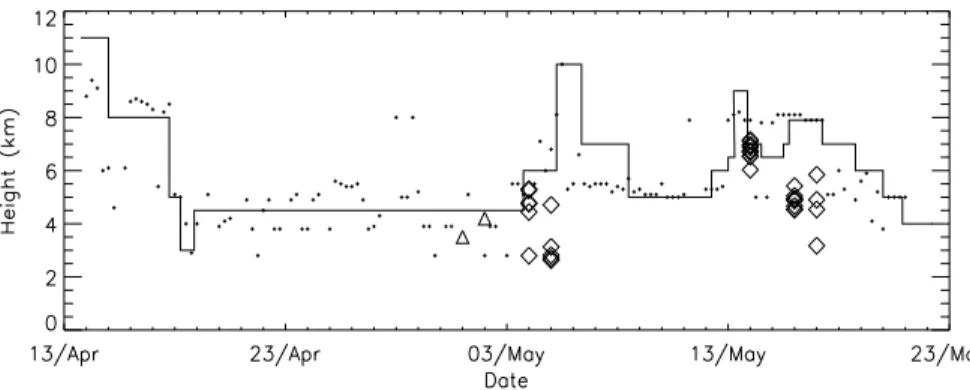
Figure 1 shows an estimate of the time varying eruption plume heights (above mean sea level) (similar to that in Webster et al. (2012)). This estimate is based on the ad-vice from the Icelandic Meteorological Office passed to the London VAAC during the
5
eruption. It aims to broadly follow the upper estimates of the eruption height which were available at the time, while only responding to significant changes in activity. Also shown is the radar data from the Keflav´ık radar, published recently by Arason et al. (2011). The most noticeable difference between the two timeseries is that the recon-struction does not follow the short period variations seen in the radar data. During the
10
period of interest (4–17 May) the reconstruction is a reasonable representation of the height of the eruption plume. In calculating the MER using the heights in Fig. 1 no ac-count has been taken of the effect that the ambient wind can have on the height of the eruption plume (Bursik et al., 2001).
To investigate the sensitivity of the model results to the assumed emission profiles
15
simulations were performed using two different profiles. For the first set of simulations the emission of ash was assumed to be uniform between the top of the volcano and the top of the eruption plume, this will be referred to as the uniform emission profile. For the second profile the emission of ash is assumed to be concentrated at the top of the eruption plume and will be referred to as the top emission profile. In the top emission
20
profile ash is emitted uniformly over a depth of 1000 m, with the top of the layer of ash emissions corresponding to the height of the eruption plume. For both emission profiles the total erupted mass is given by Eq. (1).
3 Lidar
The lidar on the FAAM aircraft was a model ALS450 manufactured by Leosphere. It is
25
ACPD
12, 9125–9159, 2012Volcanic ash clouds
A. L. M. Grant et al.
Title Page
Abstract Introduction
Conclusions References
Tables Figures
◭ ◮
◭ ◮
Back Close
Full Screen / Esc
Printer-friendly Version Interactive Discussion
Discussion
P
a
per
|
Dis
cussion
P
a
per
|
Discussion
P
a
per
|
Discussio
n
P
a
per
|
between the emitted beam and the receiver field of view occurring about 300 m below the aircraft. For the cruise altitude of 8000 m the ash features that can be identified from the aircraft are restricted to heights below about 7700 m.
For qualitative comparison between the ash layers detected by the lidar and NAME, ash features were identified subjectively using lidar backscatter and depolarisation
ra-5
tio plots. Ash was identified as having a high backscatter with a high depolarisation ratio, indicating irregular particles. Smaller aerosols (e.g. sulphate) tend to assume a spherical shape producing high backscatter and low depolarisation ratios.
Quantitative estimates of ash concentrations in the 0.6 to 35 µm (volume equivalent) size range were obtained from the extinction coefficients derived from the lidar, after
10
accounting for the extinction fraction in this size range and specific extinction derived from particle size distributions from in situ measurements (Johnson et al., 2011). In many cases the profiles of the extinction coefficient derived from the lidar show con-siderable scatter in the vertical. To estimate column integrated mass loadings smooth profiles have been fitted by eye to extinction profiles obtained over horizontal distances
15
of approximately 15 km. In general the shape of the extinction profiles are approxi-mately Gaussian, although in many cases the profiles are slightly asymmetric about the maximum. To allow for this asymmetry Gaussian curves with different widths were fitted separately to the upper and lower parts of the lidar profiles. Where there were multiple layers Gaussian curves were fitted to each layer. The use of Gaussian curves
20
is ultimately for convenience, and it provides quantitative measures for maximum con-centrations and widths. However, it should be borne in mind that the fits to the data are not objective and hence no formal error estimates are available.
On 14 May, conditions in the ash layer were close to those needed for the nucleation of ice crystals (Marenco et al., 2011). Obvious occurrences of cirrus forming in the ash
25
ACPD
12, 9125–9159, 2012Volcanic ash clouds
A. L. M. Grant et al.
Title Page
Abstract Introduction
Conclusions References
Tables Figures
◭ ◮
◭ ◮
Back Close
Full Screen / Esc
Printer-friendly Version Interactive Discussion
Discussion
P
a
per
|
Dis
cussion
P
a
per
|
Discussion
P
a
per
|
Discussio
n
P
a
per
|
Typically the extent of the ash layers used in this study correspond to flight times of between 30 min and 1 h. In comparing the lidar results to NAME the time taken to overfly the ash layers is ignored and the output from NAME closest to the central time is used for the comparison.
4 Results
5
4.1 Ash layer properties from Lidar
The average heights of the ash features identified from the FAAM lidar are plotted in Fig. 1, where they can be compared with the estimates of the eruption plume height. Because of the travel time (listed in Table 1) the heights of observed features and the plume heights at the same time will not correspond, but it might be expected that the
10
observed height will be related to the height of the eruption plume during the previous 1–2 days. There appears to be a tendency for the heights of the ash features observed by the lidar to be up to 1 km lower than the estimated height of the eruption plume used in NAME. The tendency for lidar ash features to be at a lower height than the height of the eruption plume estimated by the radar may be a result of fluctuations in plume
15
height (Dacre et al., 2011 and Folch et al., 2011), vertical transport in the atmosphere, overshooting and subsequent fall back of the plume, errors in the assumed heights or sedimentation of particles. Since the height of the eruption plume used in NAME aims to broadly follow the upper estimates of the eruption heights, it is likely to be greater than the mean height of the eruption plume which may be more representative of the
20
height of the ash layers.
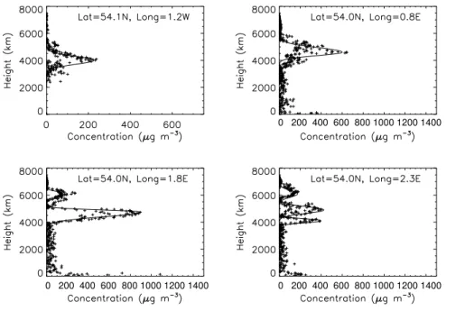
Figure 2 shows examples of the concentration profiles derived from the FAAM lidar on the 17 May together with the smooth profiles fitted to the data by eye. The aircraft track on this day was approximately west to east along 54◦N. Although the individual
estimates of concentration from the lidar show considerable scatter over a 15 km
sec-25
ACPD
12, 9125–9159, 2012Volcanic ash clouds
A. L. M. Grant et al.
Title Page
Abstract Introduction
Conclusions References
Tables Figures
◭ ◮
◭ ◮
Back Close
Full Screen / Esc
Printer-friendly Version Interactive Discussion
Discussion
P
a
per
|
Dis
cussion
P
a
per
|
Discussion
P
a
per
|
Discussio
n
P
a
per
|
On this day maximum concentrations occur at heights between 4 km and 6 km, with the peak concentrations varying between 225 µg m−3 to 900 µg m−3. Because the curves
are fitted by eye there are no formal estimates of the uncertainty in the maximum con-centration, but based on experience a reasonable estimate of the uncertainty in the fitting method is 25–50 µg m−3. At the western end of the aircraft track (Fig. 2a) there
5
is only one ash layer present while at the eastern end (Fig. 2c and d) the lidar shows multiple layers. The DLR Falcon also sampled the ash cloud on this day around 53◦N
2◦E between 16:00–17:00 UTC, i.e. about 1.5 h after the profile shown in Fig. 2(d) was
obtained. The Falcon data show the ash layer to be between 3.5 km and 6 km, with the maximum ash concentrations between 300–400 µgm−3, comparable to the FAAM lidar
10
estimates (Schumann et al., 2011).
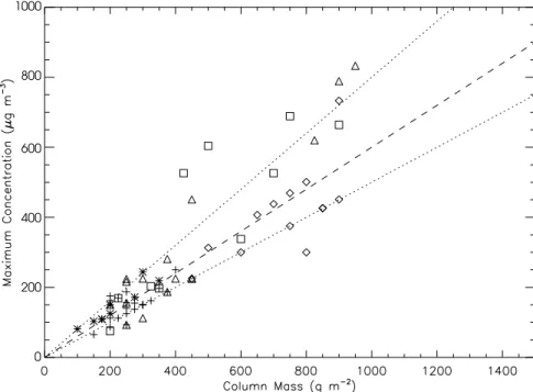
The standard deviations of the Gaussian sections that have been fitted to the lidar concentration profiles are typically around 300 m. However, to make comparisons with the NAME simulations it is useful to have a simple measure of the depth of an ash layer which does not depend on the detailed shape of the concentration profile. The
15
ratio of the integrated column mass to the maximum concentration will be used as an effective depth, leff. The effective depth can be interpreted as the depth of a layer with a constant concentration equal to the observed maximum that gives the observed column integrated mass. For a Gaussian profile with standard deviationσ,leff=√2πσ. Figure 3 shows the maximum concentrations obtained from the lidar as a function of
20
the column integrated mass, estimated from the Gaussian profiles. The multiple layers seen in some of the profiles on the 17 May have been treated as a single layer. The effective depth of the ash layers detected by the lidar is generally between 500 m–800 m which is about 10–20 % of the rise height of the eruption plume. The thickness of the ash layers observed by the lidar are comparable to thicknesses estimated by Scollo
25
ACPD
12, 9125–9159, 2012Volcanic ash clouds
A. L. M. Grant et al.
Title Page
Abstract Introduction
Conclusions References
Tables Figures
◭ ◮
◭ ◮
Back Close
Full Screen / Esc
Printer-friendly Version Interactive Discussion
Discussion
P
a
per
|
Dis
cussion
P
a
per
|
Discussion
P
a
per
|
Discussio
n
P
a
per
|
what appear as relatively thin ash layers observed by the lidar may reflect the depth of the near source eruption plume. If this is the case then it suggests that vertical turbulent diffusion within the troposphere was not important during transport (or was partly balanced by thinning of the layers due to shear).
4.2 Simulated ash clouds: horizontal structure
5
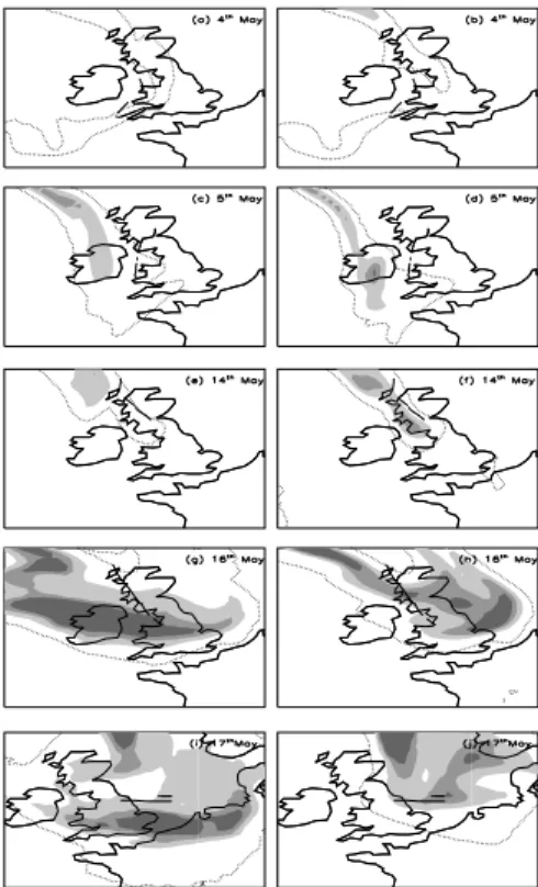
Figures 4a–j show contour plots of ash concentrations obtained from NAME, averaged from the surface to 8000 m, for each of the flights. The figures on the left show results obtained with a uniform emissions profile and Figs. 4f–j show results for the top emis-sion profile. The locations of the ash features detected by the FAAM lidar are marked by the line segments.
10
On the 4, 5 and 14 May the locations of the areas of highest ash concentrations in the NAME simulations are not particularly sensitive to the assumptions about the ash emission profile, although the actual concentrations do depend on the emission profile. This is particularly evident on the 14 May (Figs. 4e and f) when the maximum concentrations over western Scotland and northwest England are higher for the top
15
emission profile than for the uniform emission profile. The extent of the areas of low ash concentration on these days are more sensitive to the emission profile, being less extensive for the top emission profile. The flights on the 4 and 5 May took place in areas of low ash concentrations in the NAME simulations, so quantitative comparison with the lidar data on these days is likely to be sensitive to the assumed emission profiles.
20
The areas of high ash concentration in the NAME simulations on the 16 and 17 May are more sensitive to the form of the emission profile than on the other days studied. On both days the western boundary of the high concentration ash is further to the east in the simulations that use the top emission profile compared to the simulations that used the uniform emission profile. The boundary of the simulated ash cloud over Ireland on
25
ACPD
12, 9125–9159, 2012Volcanic ash clouds
A. L. M. Grant et al.
Title Page
Abstract Introduction
Conclusions References
Tables Figures
◭ ◮
◭ ◮
Back Close
Full Screen / Esc
Printer-friendly Version Interactive Discussion
Discussion
P
a
per
|
Dis
cussion
P
a
per
|
Discussion
P
a
per
|
Discussio
n
P
a
per
|
4.3 Simulated ash clouds: vertical structure
Vertical cross sections of the simulated ash layers are shown in figures 5a–c, 6a–c and 7a–c with the layers observed by the FAAM lidar being marked for comparison. To construct the cross sections the aircraft flight track was approximated as a series of line segments and the ash concentrations from NAME were interpolated onto these
5
segments at points separated by 10 km. For the 14 , 16 and 17 May the cross sections are almost along straight lines orientated predominantly north-south or east-west. For these flights it is convenient to use latitude or longitude as the horizontal co-ordinate. On the 4 and 5 May the aircraft heading varies while flying over the ash cloud and for these cross sections the horizontal co-ordinate is distance from a point on the flight
10
track before the ash was encountered. Distances are taken along the aircraft flight track from this point.
A general feature of the cross sections through the simulated ash clouds is that they show layering, either single layers (e.g. 14, 17 May, Fig. 6) or multiple layers (e.g. 5 May (Fig. 5b) or 16 May (Fig. 7b)). The presence of layers in the simulations does not
15
appear to depend on the details of the emission profile, with layers present in both sets of simulations. The simulated ash layers appear to correspond reasonably well to observed ash layers, although they are generally thicker than the observed layers.
On the 4 and 5 May the lidar detected ash layers at heights of around 3 km and 5 km and the NAME simulations using a uniform emission profile also indicates the presence
20
of ash at both heights. On the 4 May the observed ash is in patches which are typically about 100 km long, which for the layer at 3 km is much shorter than the length of layer simulated by NAME. On the 5 May the observed layers are about 200 km in length, but also appear to be less extensive than simulated layers.
The NAME simulations for the 4 and 5 May using the top emission profile do not
25
ACPD
12, 9125–9159, 2012Volcanic ash clouds
A. L. M. Grant et al.
Title Page
Abstract Introduction
Conclusions References
Tables Figures
◭ ◮
◭ ◮
Back Close
Full Screen / Esc
Printer-friendly Version Interactive Discussion
Discussion
P
a
per
|
Dis
cussion
P
a
per
|
Discussion
P
a
per
|
Discussio
n
P
a
per
|
The 5 minute radar data presented by Arason et al. (2011) suggest that the eruption plume was reaching heights of 3.5 km a.m.s.l. intermittently before the 3rd May and up to 5 km at the beginning of the 4 May. From the 5 May the height of the eruption plume remained around 5 km. From NAME the age of the simulated ash layer at 5 km is about 28 h, compared to 38 h for the layer at 3 km, so the ash in these layers was
5
emitted at different times. Although the eruption plume height used in the model does not show the intermittency apparent in the radar it does include an increase in height on the 4 May. The results from NAME suggest that some ash must have been emitted at heights below the top 1 km of the plume as the lower ash layer is captured by the simulation using the uniform emission profile but not by the simulation using the top
10
emission profile. The results from the 4 and 5 May can be considered consistent with the conclusions of Webley et al. (2009).
On the 14, 16 and 17 May (Figs. 6 and 7) the details of the vertical structure of the simulated ash clouds depend on the ash emission profile. On the 14 May the con-centrations in the simulated layer are higher using the top emission profile, compared
15
to those obtained using a uniform emission profile. On the 17 the western extent of the ash cloud appears to be better simulated using the top emission profile (compare figures 6c and 7c).
On the 16 May both of the NAME simulations show a layer that appears to corre-spond to the observed ash layer but which, in both simulations, is too far south.
Schu-20
mann et al. (2011) comment that the London VAAC forecasts on this day showed the ash to be further south than observed by the DLR Falcon or SEVIRI. It is interesting that the same error appears in the present simulations which use analysed winds. This location error is probably caused by the cumulative effect of errors in the driving mete-orology en route similar to those found for the earlier period of the eruption in Dacre et
25
ACPD
12, 9125–9159, 2012Volcanic ash clouds
A. L. M. Grant et al.
Title Page
Abstract Introduction
Conclusions References
Tables Figures
◭ ◮
◭ ◮
Back Close
Full Screen / Esc
Printer-friendly Version Interactive Discussion
Discussion
P
a
per
|
Dis
cussion
P
a
per
|
Discussion
P
a
per
|
Discussio
n
P
a
per
|
Overall the comparison between the simulations and lidar results for 14 to 17 suggest that the best match with the observed ash layers is obtained by assuming that the emission of ash is concentrated at the top of the eruption plume. For the 4 and 5 May a uniform source appears to give the best results. On the 4 May, although the eruption was beginning to re-intensify, the SEVIRI ash retrievals do not indicate the presence
5
of a sustained ash plume (Thomas and Prata, 2011). The weak and fluctuating nature of the eruption plume during the period prior to the 5 May and the change to more stable eruption activity during the period after 5 May (Petersen, 2010) may explain this difference.
4.4 Quantitative comparison between lidar and NAME
10
On the 4 May the correspondence between the observed and simulated ash layers is poor in comparison to the other days. This may be partly due to the NAME plume being positioned a little too far to the west, as is suggested by the comparison between the NAME plume position and satellite derived SO2 presented by Thomas and Prata (2011), assuming that the ash and SO2 are co-located. Because of this the results 15
from this day will not be considered further. For the other days the correspondence between the observed ash layers and the ash layers in the NAME simulations suggests that quantitative comparisons between NAME and the lidar should be made for the individual layers. Since the ash layer thicknesses differ the column integrated mass loadings (CIML) are compared since they are not sensitive to the details of the vertical
20
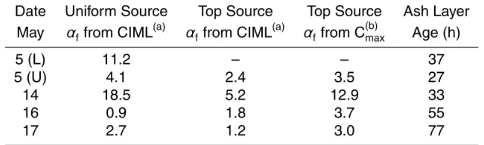
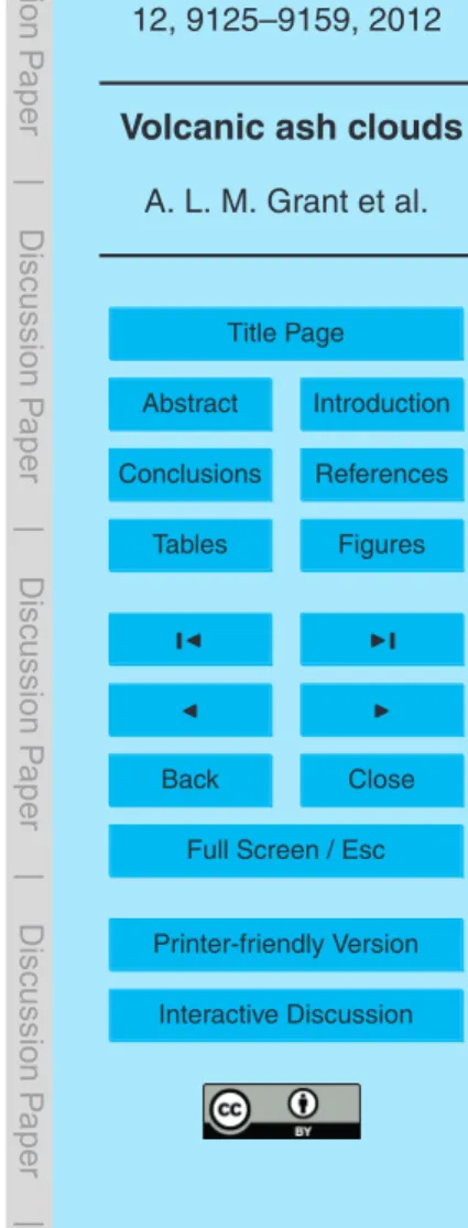
structure. Fig. 8 show the CIMLs obtained from NAME along the cross sections in Figs. 5, 6 and 7 compared to the mass loadings estimated from the lidar. The distal fine ash fraction defined in Eq. (2) has been estimated by scaling the mass loadings obtained from NAME so as to match the lidar estimates. Table 1 lists the values ofαf for both sets of NAME simulations.
25
ACPD
12, 9125–9159, 2012Volcanic ash clouds
A. L. M. Grant et al.
Title Page
Abstract Introduction
Conclusions References
Tables Figures
◭ ◮
◭ ◮
Back Close
Full Screen / Esc
Printer-friendly Version Interactive Discussion
Discussion
P
a
per
|
Dis
cussion
P
a
per
|
Discussion
P
a
per
|
Discussio
n
P
a
per
|
cloud using the uniform source. In particular the maximum in the column integrated mass load around 400 km along track in the simulated ash cloud does not appear to correspond to any feature seen by the lidar. However, using a top source in NAME, the ash layer at 3 km is missing entirely in the simulation. Therefore, at least some ash must be emitted below 3.5 km for the 3 km ash layer to be simulated in NAME. The weak and
5
intermittent nature of the eruption plume on the 4 May (Thomas and Prata, 2011) may provide the explanation for the overestimation of ash 400 km along track in the uniform source NAME simulation. With the uniform emission profile ash will have been emitted at 3 km for a longer period in the NAME simulation than would be expected to have actually occurred, which could lead to a more extensive ash layer.
10
The short horizontal line in Fig. 8c marks a region where the observed ash layer becomes very thin and the column loading of ash is negligible. (Note that the NAME simulated ash layer has been shifted 3◦N in order to perform the quantitative
compari-son. This shift accounts for the fact that the NAME simulated cloud is too far south, as discussed in Sect. 4.3). The results from NAME do not show this gap, but vary more
15
smoothly. The smooth spatial variation of simulated ash layers is due to the resolution of the meteorological model (25 km), the smooth temporal variation of the meteoro-logical fields (updated every 3 h), the lack of rapid fluctuations in the source (in both the vertical, at least in the uniform source case, and in the time variation) and the pa-rameterisation of sub-gridscale processes. The NAME simulations appear to capture
20
variations on scales of 100–200 km.
Of all of the simulations the spatial variation in the column mass loadings from NAME appear to be the most sensitive to the assumed emission profile on the 17 May (Fig. 8d). The simulation which uses the top emission profile shows good agree-ment with the lidar estimates, with both the lidar and NAME column loadings being
25
small west of 2◦W. With the uniform emission profile the column loadings in the NAME
ACPD
12, 9125–9159, 2012Volcanic ash clouds
A. L. M. Grant et al.
Title Page
Abstract Introduction
Conclusions References
Tables Figures
◭ ◮
◭ ◮
Back Close
Full Screen / Esc
Printer-friendly Version Interactive Discussion
Discussion
P
a
per
|
Dis
cussion
P
a
per
|
Discussion
P
a
per
|
Discussio
n
P
a
per
|
Most of the values forαf from CIML listed in Table 1 are less than about 5 %, the two exceptions being αf for the lower layer on the 5 May and on the 14 May for the simulation using the uniform emission profile, which are, respectively, 11 % and 18 %. Using the top emission profile the value ofαf for the 14 May is reduced by a factor of three to ∼5 %. This change is due to the increased concentrations that occur in the
5
layer above 5 km, which are transported over Scotland and north west England, when the top emission profile is used compared to the uniform emission profile. Ash below 5 km appears to be transported to the north east, away from the UK.
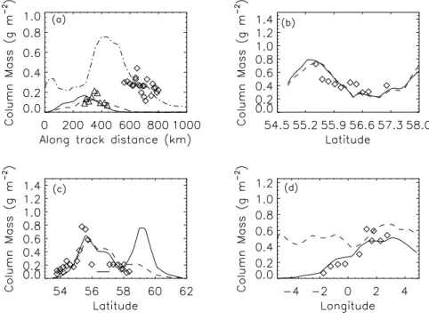
Figure 9 compares the lidar and NAME estimates of the column integrated mass taken from the simulations using the uniform emission profile for May 5 and the top
10
emission profile for 14, 16 and 17 May. A reasonable estimate of the distal fine ash fraction is 2.8 %, with of order a factor of two variation encompassing the results from most of the days. The estimates ofαf obtained in this study are in reasonable agree-ment with those obtained from ground-based lidar and NAME during the initial phase of the eruption in April (Dacre et al., 2011; Devenish et al., 2011).
15
There are few observational estimates from previous volcanic eruptions of the frac-tion of the erupted mass that survives the initial fall out phase to compare with. Wen and Rose (1994) used AVHRR (Advanced Very High Resolution Radiometer) data to estimate the mass of ash in the 13 h old ash cloud from August 1992 eruption of Spurr volcano. The ash cloud contained 0.7–0.9 % of the mass deposited at the surface.
20
Rose et al. (2000) list a number of estimates of the fine ash fraction derived from satel-lite observations of the ash clouds for a number of eruptions. For the three eruptions of Spurr in 1992 the fraction of ash remaining suspended in the atmosphere after 24 h was 0.7–2.6 %. Bearing in mind that the values ofαf obtained in this study are based on estimates of the erupted mass calculated from Eq. (1) they are consistent with the
25
ACPD
12, 9125–9159, 2012Volcanic ash clouds
A. L. M. Grant et al.
Title Page
Abstract Introduction
Conclusions References
Tables Figures
◭ ◮
◭ ◮
Back Close
Full Screen / Esc
Printer-friendly Version Interactive Discussion
Discussion
P
a
per
|
Dis
cussion
P
a
per
|
Discussion
P
a
per
|
Discussio
n
P
a
per
|
4.5 Maximum concentrations
In general the observed ash layers are thinner than the corresponding layers simulated by NAME, which will not affect the comparison of the integrated column masses, as-suming the effects of vertical wind shear are small. However, in general the maximum concentrations simulated by NAME will, when scaled using αf, underestimate actual
5
maximum concentrations. This is illustrated in Fig. 10 which shows examples of the profiles of ash concentration from the lidar and the corresponding profiles simulated by NAME, which have been scaled by the distal fine ash fraction determined from the integrated column mass. The greater depth of the simulated ash layers compared to the observed depth is clear as are the lower maximum concentrations.
10
The peak concentrations from the lidar and from the corresponding layers in the NAME simulations using the top emission profile are compared in Fig. 11. There is a reasonable correlation between the lidar and NAME for individual flights, which is simi-lar to that found for the column mass loads (see Fig. 9). These correlations suggest that the identification of the observed ash layers with ash layers in the NAME simulations
15
is justified. The ratios of lidar to NAME maximum concentrations are also listed in Ta-ble 1. They are larger than the corresponding ratios for the column integrated masses, consistent with the simulated layers being deeper than the observed ash layers (see Fig. 10). Comparison of the lidar and NAME estimates of the maximum concentration (Fig. 11) indicates that, withαf tuned on the basis of the column loads, the maximum
20
concentrations are underestimated by a factor of 1.8. This occurs because the depths of the simulated ash layers are 2–3 times larger than the observed depths.
5 Conclusions
A significant problem in modelling the the transport of volcanic ash within the atmo-sphere is the specification of the source characteristics. This study has used
obser-25
ACPD
12, 9125–9159, 2012Volcanic ash clouds
A. L. M. Grant et al.
Title Page
Abstract Introduction
Conclusions References
Tables Figures
◭ ◮
◭ ◮
Back Close
Full Screen / Esc
Printer-friendly Version Interactive Discussion
Discussion
P
a
per
|
Dis
cussion
P
a
per
|
Discussion
P
a
per
|
Discussio
n
P
a
per
|
been compared with simulations of the ash cloud obtained from the UK Met Office NAME model to constrain some properties of the ash source. The key source parame-ters are:
– The vertical profiles of the emission of ash
During the period of reasonably strong activity during mid May the best
simula-5
tions were obtained from NAME by assuming that the ash emissions are concen-trated at the top of the eruption plume. In early May as the eruption intensity was increasing assuming that ash was emitted uniformly over the depth of the erup-tion plume gave the best results. The uniform emission profile in this case was probably compensating for lack of variability in the eruption plume height used in
10
NAME compared to the actual plume height.
– The fraction of the ash that survives near source fallout and has sizes small enough to have residence times in the atmosphere of several days
Estimates of the distal fine ash fraction were in the range 2–5 %, assuming the relationship between mass eruption rate and the rise height of the eruption plume
15
is given by Eq. (1). The relatively small distal fine ash fractions are in reasonable agreement with previous values for other volcanoes obtained by estimating the erupted mass from the total mass in the ash deposited on the ground. This esti-mate of the distal fine ash fraction is also consistent with the results of Dacre et al. (2011) for the earlier phase of the eruption in April.
20
– The mass eruption rate
The sensitivity of the estimates of the mass eruption rate (MER) to the rise height of the eruption plume means that the observations of the eruption plume height have a significant impact on the present results. The simplest approach is to cal-culate the MER using Eq. (1) and the instantaneous height of the eruption plume
25
ACPD
12, 9125–9159, 2012Volcanic ash clouds
A. L. M. Grant et al.
Title Page
Abstract Introduction
Conclusions References
Tables Figures
◭ ◮
◭ ◮
Back Close
Full Screen / Esc
Printer-friendly Version Interactive Discussion
Discussion
P
a
per
|
Dis
cussion
P
a
per
|
Discussion
P
a
per
|
Discussio
n
P
a
per
|
MER or use the maximum height of the eruption plume over a given time to cal-culate the maximum MER. If observations are infrequent, or missing (e.g. radar being obscured by precipitation, Arason et al., 2011) then persistence may need to be used or some reversion to a recent average or maximum value to fill in the gaps. These methods will give different values of MER and subsequently of the
5
estimated distal fine ash fraction. For example, the MER calculated from Eq. 1 using the mean height over a six hour period (from the Keyflav´ık radar) were on average a factor of two smaller than the MER used in this study. A further com-plication is that the data underlying Eq. 1 does not involve highly time-resolved estimates of plume height.
10
The present study has assumed a simple way of specifying the eruption source for a volcanic ash transport and dispersion model. More sophisticated treatments of the eruption plume are also possible. Folch et al. (2011) used an explicit plume model to characterise the eruption source. An advantage of using a plume model is that the effects of meteorology on the rise of the eruption plume can be accounted for in
calcu-15
lating the mass eruption rate. The present, rather simple treatment, forms a benchmark against which added complexity of a more sophisticated plume model can be judged.
Acknowledgements. The authors would like to thank Steve Sparks for helpful discussions on microphysical processes in volcanic clouds and for comments on the manuscript. We would also like to thank Helen Webster and Matthew Hort at the Met Office for useful feedback on
20
the manuscript. Alan Grant was funded by a National Centre for Atmospheric Science (NCAS) national capability grant. Airborne data was obtained using the BAe-146-301 Atmospheric Re-search Aircraft (ARA) flown by Directflight Ltd and managed by the Facility for Airborne Atmo-spheric Measurements (FAAM), which is a joint entity of the Natural Environment Research Council (NERC) and the Met Office.
ACPD
12, 9125–9159, 2012Volcanic ash clouds
A. L. M. Grant et al.
Title Page
Abstract Introduction
Conclusions References
Tables Figures
◭ ◮
◭ ◮
Back Close
Full Screen / Esc
Printer-friendly Version Interactive Discussion
Discussion
P
a
per
|
Dis
cussion
P
a
per
|
Discussion
P
a
per
|
Discussio
n
P
a
per
|
References
Arason, P., Petersen, G. N., and Bjornsson, H.: Observations of the altitude of the volcanic plume during the eruption of Eyjafjallaj ¨okull, April–May 2010, Earth Syst. Sci. Data. 3, 9–17, 2011. 9131, 9137, 9143, 9149
Ansmann, A., Tesche, M., Gross, S., Freudenthaler, V., Seifert, P., Hiebsch, A., Schmidt, J.,
5
Wandinger, U., Mattis, I., M ¨uller, D., and Wiegener, M.: The 16 April 2010 major volcanic ash plume over central Europe: EARLINET lidar and AERONET photometer observations at Leipzig and Munich Germany, Geophys. Res. Lett., 37, L13810, doi:10.1029/2010GL043809, 2010. 9128
Bursik, M.: Effect of wind on the rise height of volcanic plumes, Geophys. Res. Lett., 18, 3621–
10
3624, 2001. 9131
Carey, S. and Sparks, S.: Quantitative models of the fallout and dispersal of tephra from volcanic eruption columns, Bull. Volc., 48, 109–125, 1986. 9134
Dacre, H. F., Grant, A. L. M., Hogan, R. J., Belcher, S. E., Thomson, D. J., Devenish, B., Marenco, F., Hort, M., Haywood, J. M., Ansmann, A., Mattis, I., and Clarisse, L.: Evaluating
15
the structure and magnitude of the ash plume during the initial phase of the 2010 Eyjaf-jallaj ¨okull eruption using lidar observations and NAME simulations, J. Geophys. Res., 116, D00U03, doi:10.1029/2011JD015608, 2011. 9129, 9130, 9133, 9137, 9140, 9142
Dacre, H. F., Grant, A. L. M., Thomson, D. J., and Johnson, B. T.: Observations and model simulations of column integrated mass and grain size distribution in the Eyjafjallaj ¨okull ash
20
cloud, in preparation, 2012. 9129
Devenish, B. J., Thomson, D. J., Marenco, F., Leadbetter, S. J., Ricketts, H., and Dacre, H. F.: A study of the arrival over the United Kingdom in April of the Eyjafjallaj ¨okull ash cloud using ground-based lidar and numerical simulations, Atmos. Environ., 48, 152–164, 2011. 9140 Eckhardt, S., Prata, A. J., Seibert, P., Stebel, K., and Stohl, A.: Estimation of the vertical
pro-25
file of sulfur dioxide injection into the atmosphere by a volcanic eruption using satellite col-umn measurements and inverse transport modeling, Atmos. Chem. Phys., 8, 3881–3897, doi:10.5194/acp-8-3881-2008, 2008. 9127
Flentje, H., Claude, H., Elste, T., Gilge, S., K ¨ohler, U., Plass-D ¨ulmer, C., Steinbrecht, W., Thomas, W., Werner, A., and Fricke, W.: The Eyjafjallaj ¨okull eruption in April 2010 – detection
30
ACPD
12, 9125–9159, 2012Volcanic ash clouds
A. L. M. Grant et al.
Title Page
Abstract Introduction
Conclusions References
Tables Figures
◭ ◮
◭ ◮
Back Close
Full Screen / Esc
Printer-friendly Version Interactive Discussion
Discussion
P
a
per
|
Dis
cussion
P
a
per
|
Discussion
P
a
per
|
Discussio
n
P
a
per
|
Folch, A., Costa, A., and Basart, S.: Validation of the FALL3D ash dispersion model using observations of the 2010 Eyafjallaj ¨okull volcanic ash clouds, Atmos. Environ., 48, 165–183, 2012. 9133, 9143
Heffter, J. L. and Stunder, B. J. B.: Volcanic Ash Forecast Transport and Dispersion (VAFTAD) Model, Weather Forecast, 8, 534–541, 1993. 9130
5
Johnson, B.T., Turnbull, K. F., Dorsey, J., Baran, A. K.,Ulanowski, Z., Hesse, E., Cotton, R., Brown, P. R. A., Burgess, R., Capes, G., Webster,H. N., Woolley, A. M., Rosenberg P. D. and Haywood, J. M.: In situ observations of volcanic ash clouds from the FAAM aircraft during the eruption of Eyjafjallaj ¨okull in 2010, J. Geophys. Res., in review, 2011. 9128, 9129, 9132 Jones, A. R., Thomson, D. J., Hort, M., and Devenish, B.: The U.K. Met Office’s next-generation
10
atmospheric dispersion model NAME III, edited by: Borrego, C., Air Pollution Modelling and its Application XVII, Proceedings of the 27 NATO/CCMS International Technical Meeting on Air Pollution Modelling and its Application, Springer, 580–589, 2007. 9127, 9128
Kristiansen, N. I., Stohl, A., Prata, A. J., Richter, A., Eckhardt, S., Seibert, P., Hoffmann, A., Ritter, C., Bitar, L., Duck, T. J., and Stebel, K.: Remote sensing and inverse transport
mod-15
elling of the Kasatochi eruption sulphur dioxide cloud, J. Geophys. Res., 115, D00L16, doi:10.1029/2009/2009JD013286, 2010. 9127
Marenco, F., Johnson, B., Turnbull, K., Newman, S., Haywood, J., Webster, H., and Ricketts, H.: Airborne lidar observations of the 2010 Eyjafjallaj ¨okull volcanic ash plume, J. Geophys. Res., 116, D00U05, doi:10.1029/2011JD016396, 2011. 9131, 9132
20
Mastin, L. G., Guffianti, M., Servranckx, R., Webley, P. W., Barsottie, S., Dean, K., Denlinger, R., Durant, A., Ewert, J. W., Gardner, C. A., Holliday, A. C., Neri, A., Rose, W. I., Schneider, D., Siebert, L., Stunder, B., Swanson, G., Tupper, A., Volentik, A., and Waythomas, C. F.: A multidisciplinary effort to assign realistic source parameters to model of volcanic ash-cloud transport and dispersion during eruptions, J. Volcanol. Geoth. Res., 186, 10–21, 2009. 9128,
25
9130
Petersen, G. N.: A short meteorological overview of the Eyjafjallaj ¨okull eruption 14 April–23 May 2010, Weather, 65, 203–207, doi:10.1002/wea.634, 2010. 9138
Rauthe-Sch ¨och, A., Weigelt, A., Hermann, M., Martinsson, B. G., Baker, A. K., Heue, K.-P., Brenninkmeijer, C. A. M., Zahn, A., Scharffe, D., Eckhardt, S., Stohl, A., and van Velthoven,
30
ACPD
12, 9125–9159, 2012Volcanic ash clouds
A. L. M. Grant et al.
Title Page
Abstract Introduction
Conclusions References
Tables Figures
◭ ◮
◭ ◮
Back Close
Full Screen / Esc
Printer-friendly Version Interactive Discussion
Discussion
P
a
per
|
Dis
cussion
P
a
per
|
Discussion
P
a
per
|
Discussio
n
P
a
per
|
Rose, W. I., Bluth, G. J. S., and Ernst, G. G. J.: Integrating retrievals of volcanic cloud charac-teristics from satellite remote sensors: a summary, Phil. Trans. R. Soc. Lond. A, 358, 1585– 1606, 2000. 9129, 9130, 9140
Schumann, U., Weinzierl, B., Reitebuch, O., Schlager, H., Minikin, A., Forster, C., Baumann, R., Sailer, T., Graf, K., Mannstein, H., Voigt, C., Rahm, S., Simmet, R., Scheibe, M., Lichtenstern,
5
M., Stock, P., R ¨uba, H., Sch ¨auble, D., Tafferner, A., Rautenhaus, M., Gerz, T., Ziereis, H., Krautstrunk, M., Mallaun, C., Gayet, J.-F., Lieke, K., Kandler, K., Ebert, M., Weinbruch, S., Stohl, A., Gasteiger, J., Groß, S., Freudenthaler, V., Wiegner, M., Ansmann, A., Tesche, M., Olafsson, H., and Sturm, K.: Airborne observations of the Eyjafjalla volcano ash cloud over Europe during air space closure in April and May 2010, Atmos. Chem. Phys., 11, 2245–2279,
10
doi:10.5194/acp-11-2245-2011, 2011. 9128, 9134, 9137
Scollo, S., Folch, A., Coltelli, M., and Realmuto, V. J.: Three-dimensional volcanic aerosol dis-persal: A comparison between Multiangle Imaging Spectroradiaometer (MISR) data and numerical simulations, J. Geophys. Res., 115, D24210, doi:10.1029/2009JD013162, 2010. 9134
15
Sparks, R. S., Bursik, J. M., Carey, S. N., Gilbert, J. S., Glaze, L. S., Siggurdsson, H., and Woods, A. W.: Volcanic Plumes, John Wiley and Sons. Chichester, UK, 1997. 9130
Stohl, A., Prata, A. J., Eckhardt, S., Clarisse, L., Durant, A., Henne, S., Kristiansen, N. I., Minikin, A., Schumann, U., Seibert, P., Stebel, K., Thomas, H. E., Thorsteinsson, T., Tørseth, K., and Weinzierl, B.: Determination of time- and height-resolved volcanic ash emissions and
20
their use for quantitative ash dispersion modeling: the 2010 Eyjafjallaj ¨okull eruption, Atmos. Chem. Phys., 11, 4333–4351, doi:10.5194/acp-11-4333-2011, 2011. 9127
Thomas, H. E. and Prata, A. J.: Sulphur dioxide as a volcanic ash proxy during the April– May 2010 eruption of Eyjafjallaj ¨okull Volcano, Iceland, Atmos. Chem. Phys., 11, 6871–6880, doi:10.5194/acp-11-6871-2011, 2011. 9138, 9139
25
Webley, P. W., Atkinson, D., Collins, R. L., Dean, K., Fochesatto, J., Sassen, K., Cahill, C. F., Prata, A., Flynn, C. J. and Mizutani, K.: Predicting and validating the tracking of a volcanic ash cloud during the 2006 eruption of Mt Augustine Volcano, Bull. Amer. Meteorol. Soc., 89, 1647–1658, 2008.
Webley, P. W., Stunder, B. J. B. and Kean, K. G.: Preliminary sensitivity study of eruption source
30
ACPD
12, 9125–9159, 2012Volcanic ash clouds
A. L. M. Grant et al.
Title Page
Abstract Introduction
Conclusions References
Tables Figures
◭ ◮
◭ ◮
Back Close
Full Screen / Esc
Printer-friendly Version Interactive Discussion
Discussion
P
a
per
|
Dis
cussion
P
a
per
|
Discussion
P
a
per
|
Discussio
n
P
a
per
|
Webster, H. N., Thomson, D. J., Johnson, B. T., Heard, I. P. C., Turnbull, K. F., Marenco, F., Kristiansen, N. I., Dorsey, J. R., Minikin, A., Weinzierl, B., Schumann, U., Sparks, S. S. J., Loughlin S. C., Hort, M., Leadbetter, S. J., Devenish, B., Manning, A. J., Witham, C., Haywood, J. M. and Golding, B.: Operational prediction of ash concentrations in the dis-tal volcanic cloud from the 2010 Eyjafjallaj ¨okull eruption, J. Geophys. Res., 117, D00U08,
5
doi:10.1029/2011JD016790, 2012. 9131
Wen, S. and Rose, W. I.: Retrieval of sizes and total masses of particles in volcanic clouds using AVHRR bands 4 and 5, J. Geophys. Res., 99, 5421–5431, 1994.
ACPD
12, 9125–9159, 2012Volcanic ash clouds
A. L. M. Grant et al.
Title Page
Abstract Introduction
Conclusions References
Tables Figures
◭ ◮
◭ ◮
Back Close
Full Screen / Esc
Printer-friendly Version Interactive Discussion
Discussion
P
a
per
|
Dis
cussion
P
a
per
|
Discussion
P
a
per
|
Discussio
n
P
a
per
|
Table 1. Estimates of distal fine ash fraction,αf (%). (U) is the upper layer on the 5 May and (L) is the lower layer on the 5 May.
Date Uniform Source Top Source Top Source Ash Layer May αffrom CIML(a) αffrom CIML(a) αffrom C(b)max Age (h)
5 (L) 11.2 – – 37
5 (U) 4.1 2.4 3.5 27 14 18.5 5.2 12.9 33
16 0.9 1.8 3.7 55
17 2.7 1.2 3.0 77
ACPD
12, 9125–9159, 2012Volcanic ash clouds
A. L. M. Grant et al.
Title Page
Abstract Introduction
Conclusions References
Tables Figures
◭ ◮
◭ ◮
Back Close
Full Screen / Esc
Printer-friendly Version Interactive Discussion
Discussion
P
a
per
|
Dis
cussion
P
a
per
|
Discussion
P
a
per
|
Discussio
n
P
a
per
|
0 200 400 600 800 1000 1200 1400 0 200 400 600 800 1000 1200 1400 0 200 400 600 800 1000 1200 1400
ACPD
12, 9125–9159, 2012Volcanic ash clouds
A. L. M. Grant et al.
Title Page
Abstract Introduction
Conclusions References
Tables Figures
◭ ◮
◭ ◮
Back Close
Full Screen / Esc
Printer-friendly Version Interactive Discussion
Discussion
P
a
per
|
Dis
cussion
P
a
per
|
Discussion
P
a
per
|
Discussio
n
P
a
per
|
0 200 400 600 800 1000
ACPD
12, 9125–9159, 2012Volcanic ash clouds
A. L. M. Grant et al.
Title Page
Abstract Introduction
Conclusions References
Tables Figures
◭ ◮
◭ ◮
Back Close
Full Screen / Esc
Printer-friendly Version Interactive Discussion
Discussion
P
a
per
|
Dis
cussion
P
a
per
|
Discussion
P
a
per
|
Discussio
n
P
a
per
|
Fig. 4. Column integrated mass loadings simulated by NAME. The figures on the left show simulations where the emission profiles is assumed uniform between the top of the volcano and the top of the eruption plume, figures on the right are for an emission profile concentrated at the top of the eruption plume. The dotted contour corresponds to a column integrated mass loading of 0.2 g m−2and the filled contours to 10, 20 and 30 g m−2(note these concentrations
ACPD
12, 9125–9159, 2012Volcanic ash clouds
A. L. M. Grant et al.
Title Page
Abstract Introduction
Conclusions References
Tables Figures
◭ ◮
◭ ◮
Back Close
Full Screen / Esc
Printer-friendly Version Interactive Discussion
Discussion
P
a
per
|
Dis
cussion
P
a
per
|
Discussion
P
a
per
|
Discussio
n
P
a
per
|
Fig. 5. Cross sections of ash concentration taken along aircraft tracks from NAME simulations for the 4 and 5 May.(a)4 May, uniform emission profile(b)5 May, uniform emission profile and
(c)5 May, emissions at top of plume. The darkest grey shaded areas show the outlines of ash features identified by the lidar. The dotted contour corresponds to a concentration of 2 µg m−3,
the filled contours to 20, 100, and 200 µg m−3 (note these concentrations do not a ccount for
ACPD
12, 9125–9159, 2012Volcanic ash clouds
A. L. M. Grant et al.
Title Page
Abstract Introduction
Conclusions References
Tables Figures
◭ ◮
◭ ◮
Back Close
Full Screen / Esc
Printer-friendly Version Interactive Discussion
Discussion
P
a
per
|
Dis
cussion
P
a
per
|
Discussion
P
a
per
|
Discussio
n
P
a
per
|
Fig. 6. Cross sections of ash concentration taken along aircraft tracks for simulations with a uniform emission profile. (a) 14 May, (b) 16 May and (c) 17 May. The darkest grey shaded areas show the outlines of ash features identified by the lidar. The dotted contour corresponds to a concentration of 20 µg m−3, the filled contours to 200, 1000, and 2000 µg m−3(note these
ACPD
12, 9125–9159, 2012Volcanic ash clouds
A. L. M. Grant et al.
Title Page
Abstract Introduction
Conclusions References
Tables Figures
◭ ◮
◭ ◮
Back Close
Full Screen / Esc
Printer-friendly Version Interactive Discussion
Discussion
P
a
per
|
Dis
cussion
P
a
per
|
Discussion
P
a
per
|
Discussio
n
P
a
per
|
Fig. 7. Cross sections of ash concentration taken along aircraft tracks for simulations with emissions concentrated at the top of the eruption plume.(a) 1 May, (b) 16 May and (c) 17 May. The darkest grey shaded areas show the outlines of ash features identified by the lidar. The dotted contour corresponds to a concentration of 20 µg m−3, the filled contours to 200,
1000, and 2000 µg m−3(note these concentrations do not account for fall out of ash near the
ACPD
12, 9125–9159, 2012Volcanic ash clouds
A. L. M. Grant et al.
Title Page
Abstract Introduction
Conclusions References
Tables Figures
◭ ◮
◭ ◮
Back Close
Full Screen / Esc
Printer-friendly Version Interactive Discussion
Discussion
P
a
per
|
Dis
cussion
P
a
per
|
Discussion
P
a
per
|
Discussio
n
P
a
per
|
Fig. 8. Comparisons between lidar estimates of column mass loads and NAME estimates.
(a)Column mass estimates for the 3 km layer on the 5 May (diamonds) and the 5 km layer on the 5 May (triangles), as shown in Fig. 5. NAME column mass using uniform emissions for the ash layer at 3 km (dot-dashed line), NAME column mass for ash layer at 5 km for top source (solid line), NAME column mass for ash layer at 5 km for uniform emissions (dashed line). The NAME results are scaled to fit the observations.(b) Lidar column mass estimates on the 14 (diamonds). NAME column mass for top source (solid line) and uniform emissions (dashed line). The NAME results have been scaled to match the observations.(c)as(b)but for 16 May.
ACPD
12, 9125–9159, 2012Volcanic ash clouds
A. L. M. Grant et al.
Title Page
Abstract Introduction
Conclusions References
Tables Figures
◭ ◮
◭ ◮
Back Close
Full Screen / Esc
Printer-friendly Version Interactive Discussion
Discussion
P
a
per
|
Dis
cussion
P
a
per
|
Discussion
P
a
per
|
Discussio
n
P
a
per
|
0 200 400 600 800 1000 1200 1400
0 200 400 600 800 1000 1200 1400 0 200 400 600 800 1000 1200 1400
0 200 400 600 800 1000 1200 1400
ACPD
12, 9125–9159, 2012Volcanic ash clouds
A. L. M. Grant et al.
Title Page
Abstract Introduction
Conclusions References
Tables Figures
◭ ◮
◭ ◮
Back Close
Full Screen / Esc
Printer-friendly Version Interactive Discussion
Discussion
P
a
per
|
Dis
cussion
P
a
per
|
Discussion
P
a
per
|
Discussio
n
P
a
per
|
0 175 350 525 700 875
−3
NAME Max Conc ( g m )