www.atmos-chem-phys.net/12/10145/2012/ doi:10.5194/acp-12-10145-2012
© Author(s) 2012. CC Attribution 3.0 License.
Chemistry
and Physics
Horizontal and vertical structure of the Eyjafjallaj¨okull ash cloud
over the UK: a comparison of airborne lidar observations
and simulations
A. L. M. Grant1, H. F. Dacre1, D. J. Thomson2, and F. Marenco2
1Department of Meteorology, University of Reading, Reading, UK 2Met Office, Exeter, UK
Correspondence to:H. F. Dacre ([email protected])
Received: 20 February 2012 – Published in Atmos. Chem. Phys. Discuss.: 10 April 2012 Revised: 22 August 2012 – Accepted: 27 October 2012 – Published: 5 November 2012
Abstract. During April and May 2010 the ash cloud from the eruption of the Icelandic volcano Eyjafjallaj¨okull caused widespread disruption to aviation over northern Europe. The location and impact of the eruption led to a wealth of ob-servations of the ash cloud were being obtained which can be used to assess modelling of the long range transport of ash in the troposphere. The UK FAAM (Facility for Airborne Atmospheric Measurements) BAe-146-301 research aircraft overflew the ash cloud on a number of days during May. The aircraft carries a downward looking lidar which detected the ash layer through the backscatter of the laser light. In this study ash concentrations derived from the lidar are compared with simulations of the ash cloud made with NAME (Nu-merical Atmospheric-dispersion Modelling Environment), a general purpose atmospheric transport and dispersion model. The simulated ash clouds are compared to the lidar data to determine how well NAME simulates the horizontal and ver-tical structure of the ash clouds. Comparison between the ash concentrations derived from the lidar and those from NAME is used to define the fraction of ash emitted in the eruption that is transported over long distances compared to the to-tal emission of tephra. In making these comparisons possible position errors in the simulated ash clouds are identified and accounted for.
The ash layers seen by the lidar considered in this study were thin, with typical depths of 550–750 m. The vertical structure of the ash cloud simulated by NAME was generally consistent with the observed ash layers, although the layers in the simulated ash clouds that are identified with observed ash layers are about twice the depth of the observed layers. The
structure of the simulated ash clouds were sensitive to the profile of ash emissions that was assumed. In terms of hori-zontal and vertical structure the best results were obtained by assuming that the emission occurred at the top of the erup-tion plume, consistent with the observed structure of eruperup-tion plumes. However, early in the period when the intensity of the eruption was low, assuming that the emission of ash was uniform with height gives better guidance on the horizontal and vertical structure of the ash cloud.
Comparison of the lidar concentrations with those from NAME show that 2–5 % of the total mass erupted by the vol-cano remained in the ash cloud over the United Kingdom.
1 Introduction
The eruption of the Icelandic volcano Eyjafjallaj¨okull during April and May 2010 lead to the widespread disruption of air travel throughout Europe due to the hazard posed to aircraft by volcanic ash. At various times during this period parts of European airspace were closed, leading to significant fi-nancial losses by airlines and leaving millions of passengers stranded throughout the world.
the trajectories of particles originating at the position of the volcano to determine where the volcanic ash cloud is trans-ported. Webster et al. (2012) give details about the forecast-ing of the ash clouds usforecast-ing NAME durforecast-ing the eruption.
A major uncertainty in modelling volcanic ash clouds with volcanic ash transport and dispersion (VATD) models, such as NAME, is the specification of the eruption source param-eters (ESP). A VATD model needs information on basic pa-rameters such as the height of the eruption plume, the mass eruption rate and the vertical distribution of the emitted mass. The sensitivity of predictions of ash dispersal to the emission profile has been investigated by Webley et al. (2009) for the August 1992 eruption of Mount Spurr. Their study found that the areal extent of the simulated ash cloud was sensitive to assumptions about the emission profile, with the best agree-ment between the simulations and satellite observations of the extent of the ash cloud obtained using emission profiles which have releases at all heights within the eruption column. Eckhardt et al. (2008) and Kristiansen et al. (2010) de-scribe a data assimilation approach to obtain the emission profile of sulphur dioxide for the eruptions of Jebel el Tair and Kasatochi respectively using satellite retrievals of total column sulphur dioxide and a VATD model. Recently Stohl et al. (2011) and Kristiansen et al (2012) have extended this approach to volcanic ash, using data from SEVIRI (Spinning Enhanced Visible Infra-Red Imager) to estimate the vertical distribution and magnitude of the emissions during the Ey-jafjallaj¨okull eruption.
An alternative to the satellite inversion approach for es-timating the volcanic emissions is to use empirical rela-tionships between the mass eruption rate (MER) and plume height (Sparks et al., 1997; Mastin et al., 2009). This was the approach used by the London VAAC during the eruption and the subsequent eruption of Grimsv¨otn in 2011 (Webster et al., 2012). Much of the ash in the eruption plume falls out close to the volcano forming the tephra blanket and to es-timate concentrations of ash at long ranges an eses-timate of the fraction of the ash that survives early fall out is needed. Previous estimates this fraction range from 0.05 % to 10 % (Mastin et al., 2009)
This study uses estimates of ash concentrations obtained around the UK by the FAAM (Facility for Airborne Atmo-spheric Measurements) BAe-146 aircraft. The ash concen-trations were estimated from lidar backscatter profiles mea-sured during five flights in May 2010. Comparisons of the horizontal and vertical structure of the ash cloud obtained from the NAME model are described and estimates of the fine ash fraction for the Eyjafjallaj¨okull eruption are made.
2 Model
NAME is a Lagrangian particle trajectory model that is de-signed for use in a range of dispersion modelling applica-tions (Jones et al., 2007; Webster et al., 2012). Particles are
released at the source, which in this case is the volcanic eruption plume. Each of the particles represents a mass of volcanic ash. Their trajectories are calculated using analy-sis wind fields, with a temporal resolution of 3 h, obtained from the global version of the Met Office Unified Model. The model particles are assumed to be carried along by the wind with the effects of turbulence represented by us-ing stochastic perturbations to the trajectories derived from a semi-empirical turbulence parameterisation. NAME also in-cludes treatments of sedimentation and dry and wet depo-sition (Dacre et al. (2011) for further details). Ash concen-trations are computed by summing the mass of particles in model grid boxes, which are 0.374◦in latitude by 0.5625◦ in longitude in the horizontal and 200 m in the vertical, over one hour. The concentration is obtained by dividing the total mass by the volume of the grid box.
Rose et al. (2000) identify three stages in the evolution of volcanic ash clouds. In the first few hours large particles fall out close to the volcano, forming the proximal tephra blan-ket. This is followed by a period, typically lasting about 24 h, in which the mass in the ash cloud decreases with time, prob-ably due to particle aggregation and subsequent fall out of the aggregates. A large fraction of the erupted mass is removed from the ash cloud during these two phases. Subsequent re-moval of ash is mainly due to meteorological processes and deposition. NAME does not represent any of the microphysi-cal processes, such as aggregation, that occur within the vol-canic ash cloud, although it does have representations of par-ticle sedimentation as well as wet and dry deposition.
The removal of ash by sedimentation depends on the size distribution of the ash particles. In situ observations of the ash cloud by the FAAM aircraft over and around the UK show that particles were generally less than 10 µm in diam-eter (Johnson et al., 2011) in the Eyjafjallaj¨okull ash cloud. Sedimentation of particles with diameters less than 10 µm has a small effect on the column mass of ash for travel times of 24 to 80 h that are relevant in this study. This has been de-termined by testing the sensitivity of the results to different particle sizes (Dacre et al., 2012). Because of this the evolu-tion of the particle size distribuevolu-tion in the ash cloud due to sedimentation has been neglected by setting the particle size to 3 µm.
Comparing the lidar observation with NAME an effective source strength for the fine ash particles which formed the ash layers seen by the lidar can be estimated. This effective source strength represents the mass eruption rate of those ash particles that are not removed from the cloud close to the volcano.
Fig. 1. Timeseries of the height of the eruption plume above sea level. Height of the eruption plume used in NAME simulations (solid line), maximum heights detected by radar (small crosses) taken from Arason et al. (2011), heights of ash layers observed by FAAM aircraft (diamonds), heights of ash layers observed by the DLR Falcon taken from Schumann et al. (2011) (triangles).
of the eruption plume and the MER is taken to be,
M=140.8H4.15 (1)
whereH is the height of the eruption plume above the vol-cano summit in kilometres andM is the rate of mass emis-sion in kilogrammes per second (Webster et al., 2012). This relationship is based on a fit to the thresholds in the lookup table designed by NOAA for the VAFTAD model (Heffter and Stunder, 1993) and calibrated by the ’Mastin’ curve to give the emission rate as a function of plume height as de-scribed by Dacre et al. (2011). For the eruption plume heights relevant to the Eyjafjallaj¨okull eruption the MER estimated from Eq. (1) is within 15 % of estimates based on the rela-tionships proposed by Sparks et al. (1997) and Mastin et al. (2009). Mastin et al. (2009) find that the MER from their pro-posed relationship and the actual MER can differ by a factor of upto 3.5 for an eruption plume height of about 6 km, so the differences between the MER predicted by the different relationships are insignificant.
The effective source strength for fine ash is assumed to be,
Mf=αf(t )140.8H4.15 (2)
whereMfis the effective rate of emission of fine ash,αfis
the fine ash fraction, i.e. the fraction of ash which does not fall out close to the volcano. In principle the fine ash fraction is a function of the age of the ash,t, due to the effects of processes that are not represented in NAME, such as aggre-gation. However, these processes are expected to have their main effects for travel times less than 24 h (Rose et al., 2000). The fine ash fraction,αfwill be estimated by comparing ash
concentrations from NAME, using Eq. (1), with those ob-tained from the lidar.
Figure 1 shows a reconstruction of the time varying erup-tion plume heights (above mean sea level) which is similar to that in Webster et al. (2012). This reconstruction is based on the advice from the Icelandic Meteorological Office passed
to the London VAAC during the eruption. It aims to broadly follow the upper estimates of the eruption height which were available at the time, while only responding to significant changes in activity. Also shown is the data from the Keflav´ık radar, published by Arason et al. (2011). The most noticeable difference between the two timeseries is that the reconstruc-tion does not follow the short period variareconstruc-tions seen in the radar data. During the period of interest (4–17 May) the re-construction is a reasonable representation of the height of the eruption plume from the radar data. In calculating the MER using the heights in Fig. 1 no account has been taken of the effect that the ambient wind can have on the height of the eruption plume (Bursik, 2001).
To investigate the sensitivity of the model results to the assumed emission profiles simulations were performed us-ing two different profiles. For the first set of simulations the emission of ash was assumed to be uniform between the top of the volcano and the top of the eruption plume, this is re-ferred to as the uniform emission profile. For the second pro-file the emission of ash is assumed to be concentrated at the top of the eruption plume and is referred to as the top emis-sion profile. In the top emisemis-sion profile ash is emitted uni-formly over a depth of 1000 m, with the top of the layer of ash emissions corresponding to the height of the eruption plume. For both emission profiles the total erupted mass is given by Eq. 1.
3 Lidar
can be identified from the aircraft are restricted to heights below about 7700 m.
Ash features were identified subjectively using lidar backscatter and depolarisation ratio plots. Ash was identified as having a high backscatter with a high depolarisation ratio, indicating irregular particles. Smaller aerosols (e.g. sulphate) tend to assume a spherical shape producing high backscatter and low depolarisation ratios (see Marenco et al. (2011) for details on the interpretation of the lidar returns).
Quantitative estimates of ash concentrations in the 0.6 to 35 µm (volume equivalent) size range were obtained from the extinction coefficients derived from the lidar, after ac-counting for the extinction fraction in this size range and spe-cific extinction derived from particle size distributions from in-situ measurements (Johnson et al., 2011; Marenco et al., 2011). The uncertainty in the concentrations is estimated to be a factor of 2.
In many cases the profiles of the ash concentration derived from the lidar show considerable scatter in the vertical. To es-timate column integrated mass loadings smooth profiles have been fitted by eye to the profiles of ash concentration ob-tained over horizontal distances of approximately 15 km. In general the concentration profiles are approximately Gaus-sian in shape, although in many cases the profiles are slightly asymmetric about the maximum. To allow for this asymme-try Gaussian curves with different widths were fitted sep-arately to the upper and lower parts of the lidar profiles. Where there were multiple layers Gaussian curves were fit-ted to each layer. The use of Gaussian curves is ultimately for convenience, and it provides quantitative measures for maxi-mum concentrations and widths. However, it should be borne in mind that the fits to the data are not objective and hence no formal error estimates are available.
On 14 May, there is evidence that there were ice particles in the ash layers (Marenco et al., 2011). Obvious occurrences of cirrus forming in the ash cloud were removed from the dataset. However, it is possible that ice nucleated ash was present in the ash cloud, which would lead to ash concen-trations being overestimated. The presence of ice was not a problem on the other days.
Typically the extent of the ash layers used in this study correspond to distances of 250–600 km and flight times of between 30 min and 1 h. The ash concentrations from NAME are obtained over one hour, which provides statistical relia-bility. In comparing the lidar results to NAME the time taken to overfly the ash layers has been ignored and the output from NAME closest to the central time is used for the comparison. Over a period of an hour the evolution of the ash clouds sim-ulated by NAME is relatively small and fixing the time in this way does not have a significant effect on the comparisons. In addition the use of NAME fields at a particular time to iden-tify features that correspond to the observed ash layers allows location errors in the simulated clouds to be assessed.
4 Results
4.1 Ash layer properties from lidar
The average heights of the ash features identified from the FAAM lidar are plotted in Fig. 1, where they can be com-pared with the estimates of the eruption plume height. Be-cause of the travel time (listed in Table 1 as ash age) the heights of observed features and the plume heights at the same time will not correspond, but it might be expected that the observed height will be related to the height of the erup-tion plume during the previous 1–3 days. There appears to be a tendency for the heights of the ash features observed by the lidar to be up to 1 km lower than the estimated height of the eruption plume used in NAME. The tendency for lidar ash features to be at a lower height than the height of the erup-tion plume estimated by the radar may be a result of fluctua-tions in plume height (Dacre et al., 2011; Folch et al., 2011), vertical transport in the atmosphere, overshooting and subse-quent fall back of the plume, errors in the assumed heights or sedimentation of particles. Since the height of the eruption plume used in NAME aims to broadly follow the upper es-timates of the eruption heights, it is likely to be greater than the mean height of the eruption plume which may be more representative of the height of the ash layers.
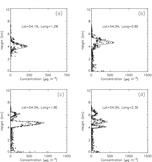
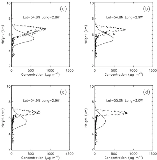
Figure 2 shows examples of the concentration profiles de-rived from the FAAM lidar on the 17 May together with the smooth profiles fitted to the data by eye. The aircraft track was approximately west to east along 54◦N. Although the in-dividual estimates of concentration from the lidar show con-siderable scatter over a 15 km section the Gaussian curves provide a reasonable approximation to the observed profiles. The maximum concentrations occur at heights between 4 km and 6 km, with the peak concentrations varying between 225 µg m−3to 800 µg m−3. Because the curves are fitted by eye there are no formal estimates of the uncertainty in the maximum concentration, but based on experience fitting the curves to the observations a reasonable estimate of the un-certainty is 25–50 µg m−3. At the western end of the aircraft track (Fig. 2a) there is only one ash layer present while at the eastern end (Fig. 2c and d) the lidar shows multiple layers.
The Cloud Aerosol Probe (CAS) on the Bae 146 measured a concentration of 400–500 µg m−3in a layer extending from 3.5–6.5 km at 14:45 UTC on 17 May (Turnbull et al , 2012). The in-situ observations do not appear to show the multi-ple layered structure at the most easterly profile in Fig. 2 which is in a similar location. The DLR Falcon also sam-pled the ash cloud on this day around 53◦N 2◦E between 16:00–17:00 UTC, i.e. about 1.5 h after the profile shown in Fig. 2d was obtained. The Falcon data show the ash layer to be between 3.5 km and 6 km, with the maximum ash concen-trations between 300–400 µg m−3, comparable to the FAAM lidar estimates (Schumann et al., 2011).
Table 1. Estimates of distal fine ash fraction,αf (%).
Date Uniform Source Top Source Top Source Ash Layer May αffrom CIMLa αffrom CIMLa αffrom Cbmax Age (h)
4 10.0 3.5 8.0 25
5(L)c 11.2 – – 37
5(U )c 4.1 2.4 3.5 27
14 18.5 5.2 12.9 33
16 0.9 1.8 3.7 55
17 2.7 1.2 3.0 77
aColumn Integrated Mass Loading bMaximum Concentration
c(U) is for the upper layer (L) is for the lower layer
Fig. 2. Examples of concentration profiles derived from lidar between 14:00 and 15:00 UTC on the 17 May. The crosses show the concen-tration estimates from the lidar, the solid curves show the Gaussian curves that have been fitted to the observations by eye.
about 300 m. However, to make comparisons with the NAME simulations it is useful to have a simple measure of the thick-ness of an ash layer which does not depend on the detailed shape of the concentration profile. The ratio of the integrated column mass to the maximum concentration will be used as an effective thickness, leff. The effective thickness can be
interpreted as the thickness of a layer with a constant
con-centration equal to the observed maximum that gives the ob-served column integrated mass. For a Gaussian profile with standard deviationσ,leff =√2π σ.
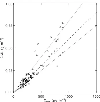
Fig. 3. Comparison between the column integrated mass load (CIML) and the maximum concentration (Cmax)for lidar
obser-vations. The dashed line corresponds to an effective depth for the ash layers of 600 m, the dotted lines are for effective depths of 500 m and 800 m. The symbols show results for different flights. 4 (crosses); 5 May (stars); 14 May (diamonds); 16 May (triangles) and 17 May (squares).
as a single layer. The effective depth of the ash layers de-tected by the lidar is generally between 500 m–800 m which is about 10–20 % of the rise height of the eruption plume. The thickness of the ash layers observed by the lidar are compa-rable to thicknesses estimated by Scollo et al. (2010) using data from MISR (Multi-angle Imaging SpectroRadiometer) for the 2001 and 2002 eruptions of Etna. The Scollo et al. (2010) results were obtained within 250 km of Etna. Carey and Sparks (1986) suggest that close to the eruption the thick-ness of the umbrella region of the ash cloud is≈0.3H. This suggests that what appear as relatively thin ash layers ob-served by the lidar probably reflect the depth of the near source eruption plume. If this is the case then it suggests that vertical turbulent diffusion within the troposphere was not important during transport (or was partly balanced by thin-ning of the layers due to shear).
4.2 Simulated ash clouds: horizontal structure
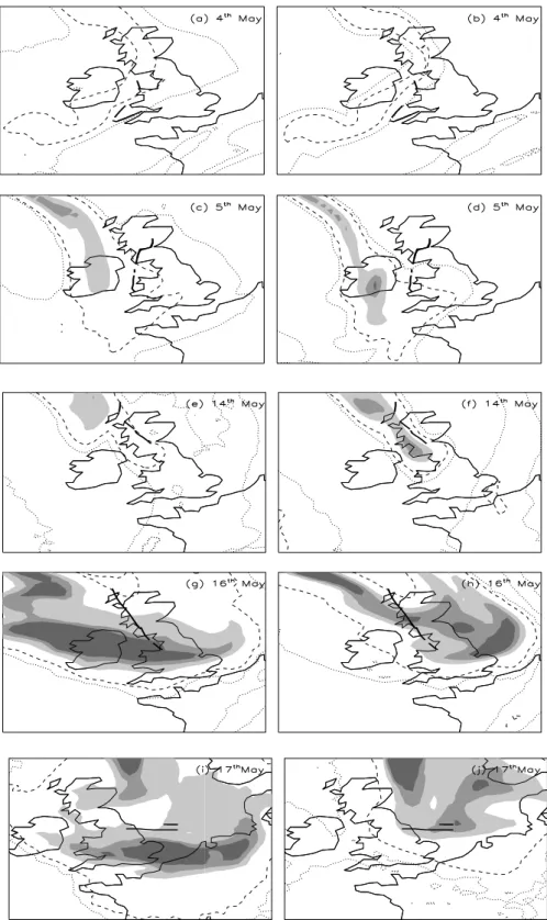
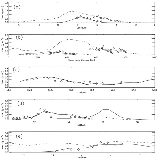
Figure 4a–j shows contour plots of the column integrated mass loadings (CIML) obtained from NAME for each of the flights. Figure 4a, c, e, g, i shows the results obtained with a uniform emission profile and Fig. 4b, d, f, h, j shows results for the top emission profile. The locations of the ash features detected by the FAAM lidar are marked by the line segments.
On the 4, 5 and 14 May the locations of the areas of high-est ash concentrations in the NAME simulations are not par-ticularly sensitive to the assumptions about the ash emission profile, although the actual concentrations do depend on the emission profile. This is particularly evident on the 14 May (Fig. 4e and f) when the maximum concentrations over west-ern Scotland and northwest England are higher for the top emission profile than for the uniform emission profile. The extent of the areas of low ash concentration on these days are more sensitive to the emission profile, being less extensive for the top emission profile. The flights on the 4 and 5 May took place in areas of low ash concentration in the NAME simulations, so quantitative comparison with the lidar data on these days is likely to be sensitive to the assumed emis-sion profiles.
The areas of high ash concentration in the NAME simu-lations on the 16 and 17 May are more sensitive to the form of the emission profile than on the other days studied. On both days the western boundary of the high concentration ash is further to the east in the simulations that use the top emission profile compared to the simulations that used the uniform emission profile. The boundary of the simulated ash cloud over Ireland on the 16 May using the top emission pro-file is consistent with the observations of Rauthe-Schoch et al. (2012). On both the 16 and 17 May the aircraft flew in the areas in which both sets of NAME simulations indicate relatively high ash concentrations.
4.3 Simulated ash clouds: vertical structure
Vertical cross sections of the simulated ash layers are shown in Figs. 5a–c, 7a–c and 8a–c with the layers observed by the FAAM lidar being marked for comparison. With the excep-tion of the 4 May the cross secexcep-tions are taken along the air-craft flight tracks, which were approximated by a series of line segments The ash concentrations from NAME were in-terpolated onto the flight tracks at points separated by 10 km. For the 14, 16 and 17 May the cross sections are almost along straight lines orientated predominantly north-south or east-west. For these flights it is convenient to use latitude or lon-gitude as the horizontal co-ordinate in the plots, although the cross sections are taken along the aircraft track. On the 4 and 5 May the aircraft heading varies while flying over the ash cloud and for these cross sections the horizontal co-ordinate is distance from a point on the flight track before the ash was encountered. Distances are taken along the aircraft flight track from this point.
Fig. 5. Cross sections of ash concentration taken along aircraft tracks from NAME simulations for the 4 and 5 May.(a)4 May, uniform emission profile(b)5 May, uniform emission profile and
(c)5 May, emissions at top of plume. The dark grey shaded areas show the outlines of ash features identified by the lidar. The dotted contour corresponds to a concentration of 2 µg m−3and is taken to show the edge of the ash cloud. The filled contours correspond to 20, 200, and 200 µg m−3(note these concentrations do not account for fall out of ash near the volcano).
correspond reasonably well to observed ash layers, although they are generally thicker.
On the 4 and 5 May the lidar detected ash layers at heights of around 3 km and 5 km. The NAME simulations using a uniform emission profile also indicates the presence of ash at both heights, although with almost zero concentration on the 4 May. The lower ash layer observed on the 5 May lies towards the edge of the NAME ash cloud, but higher concen-trations in the NAME cloud are present about 200 km to the south. With the top emission profile the NAME simulations on the 4 (plot not shown) and 5 May do not show ash layers around 3km, but the layer around 5km on the 5 May still cor-responds to a layer that is present in the NAME simulation.
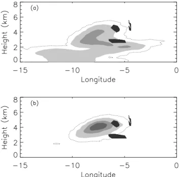
Figure 4a and b show the aircraft track on the 4 May to be close to the edge of the simulated ash cloud, particularly with the top emission profile. The relationship between the aircraft observations and model results on the 4 May is il-lustrated more clearly by an east-west cross section through the model ash cloud. The cross sections shown in Fig. 6a and b are taken along 52◦N. Note that the upper and lower ash features observed by the lidar occur at different latitudes.
The observed ash patches are towards the eastern edge of the NAME ash cloud. Thomas and Prata (2011) show sul-phur dioxide retrievals for this day which suggest that the
Fig. 6. East-West cross sections of ash concentration on 4 May along 52◦N(a)Uniform emission profile.(b)Top emission profile. Other details as Fig. 5
ash cloud may be further east than NAME indicates. Such an error would make the association between the NAME ash clouds and the observed features closer. Because of its thick-ness the NAME ash cloud obtained with the top emission source could also be considered to be associated with the ob-served ash patches. More information on the actual ash dis-tribution is needed to provide a more precise interpretation of the relationship between the observed ash features and the results from NAME.
On the 14, 16 and 17 May (Figs. 7 and 8) the details of the vertical structure of the simulated ash clouds depend on the ash emission profile. On the 14 May the concentrations in the simulated layer are higher using the top emission profile, compared to those obtained using a uniform emission pro-file. On the 17 the western extent of the ash cloud appears to be better simulated using the top emission profile (compare Figs. 7c and 8c).
Fig. 7. Cross sections of ash concentration taken along aircraft tracks for simulations with a uniform emission profile.(a)14 May,
(b)16 May and(c)17 May. Other details as Fig. 5.
this case the position of the simulated ash cloud is moved in the direction of the aircraft track so the southern edges of the simulated and observed ash layers match.
4.4 Quantitative comparison between lidar and NAME
The correspondence between the observed ash layers and the ash layers in the NAME simulations suggests that quantita-tive comparisons between NAME and the lidar can be made for the individual layers. Since the ash layer thicknesses dif-fer the column integrated mass loadings are compared since they are not sensitive to the details of the vertical structure. Figure 9 show the CIMLs obtained from NAME along the cross sections in Figs. 5, 6, 7 and 8 compared to those esti-mated from the lidar. For the 4 May the comparison between NAME and the lidar observations is done using the cross sec-tions in Fig. 6a and b rather than using the along track pro-files. The distal fine ash fraction defined in Eq. (2) has been estimated by scaling the mass loadings obtained from NAME to match the lidar estimates. The values ofαfobtained from
both sets of NAME simulations are listed in Table 1. The spatial variation of the observed column loadings and those from NAME are generally in good agreement, although there are differences. Figure 9a shows the comparisons for the 4 May along an east-west cross sections in Fig. 6. There is agreement between the variations in the observed ash mass and that derived from NAME for the 3 km feature. For the top emission profile there is reasonable agreement between the observations and NAME if it is assumed that the NAME ash cloud is about 1.5◦ too far to the west. Such an error
Fig. 8. Cross sections of ash concentration taken along aircraft tracks for simulations with emissions concentrated at the top of the eruption plume.(a)14 May,(b)16 May and(c)17 May. Other de-tails as Fig. 5.
would agree with the satellite observations in Thomas and Prata (2011).
For the 5 May Fig. 9b suggests that the ash layer at 3 km is much less extensive than the simulated ash cloud using the uniform source. In particular the maximum in the column integrated mass around 400 km in the simulated ash cloud does not appear to correspond to any feature seen by the lidar. However, using a top source in NAME, the ash layer at 3 km is missing entirely in the simulation showing that some ash must be emitted below 3.5 km for the 3 km ash layer to be simulated in NAME.
The short horizontal line in Fig. 9d marks a region where the observed ash layer becomes very thin and the column loading of ash is negligible. (Note that the ash layer simu-lated by NAME has been moved 3◦N in order to perform the quantitative comparison). The results from NAME do not show this gap, but vary more smoothly. The smooth spa-tial variation of simulated ash layers is due to the resolution of the meteorological model (25 km), the smooth temporal variation of the meteorological fields (updated every 3 h), the lack of rapid fluctuations in the source (in both the vertical, and in time) and the parameterisation of sub-gridscale pro-cesses. The NAME simulations appear to capture variations on scales of 100–200 km.
Fig. 9. Comparisons between lidar estimates of CIML and estimates from NAME.(a)Estimates of the CIML from the lidar on 4 May (diamonds) and offset by 1.5◦W (triangles). Estimates of the CIML from NAME, top source (full curve) and uniform emissions (dashed curve).(b)Estimates of the CIML for the 3 km layer on the 5 May (diamonds) and the 5 km layer (triangles). Estimates of the CIML from NAME using uniform emissions for the ash layer at 3 km (dot-dashed line), for the layer at 5 km for top source (solid line), for the uniform emissions (dashed line). The NAME results are scaled to fit the observations.(c)Lidar estimates of the CIML on the 14 (diamonds). Estimates of the CIML from NAME for top source (solid line) and uniform emissions (dashed line).(d)as(c)but for 16 May.(e)as(c)but for 17 May.
good agreement with the lidar estimates, with both the lidar and NAME column loadings being small to the west of 2◦W. With the uniform emission profile the column loadings in the NAME simulation extend much further west than observed. However, both simulations give a similar value forαfusing
the observed column loadings at the eastern end of the air-craft track.
Most of the values for αf from the comparison of the
CIMLs which are listed in Table 1 are less than about 5 %, the two exceptions beingαffor the lower layer on the 5 May and
on the 14 May for the simulation using the uniform emis-sion profile, which are, respectively, 11 % and 18 %. Using the top emission profile the value ofαffor the 14 May is
re-duced by a factor of three to∼5 %. This large change inαf
is due to the increased concentrations that occur in the layer above 5 km over Scotland and north west England, when the top emission profile is used compared to the uniform
emis-sion profile. With the uniform source ash below 5 km appears to be transported to the north east, away from the UK.
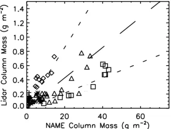
Figure 10 compares the lidar and NAME estimates of the column integrated mass taken from the simulations using the uniform emission profile for May 5 and the top emission pro-file for 14, 16 and 17 May. A reasonable estimate of the distal fine ash fraction is 2.8 %, with of order a factor of two vari-ation encompassing the results from most of the days. These estimates ofαfare in reasonable agreement with those
ob-tained from ground-based lidar and NAME during the initial phase of the eruption in April (Dacre et al., 2011; Devenish et al., 2011).
Fig. 10. Comparison between the CIMLs from NAME simulations and estimates from the FAAM lidar. The symbols are; 3 km layer 5 May (crosses); 5 km layer 5 May (stars); 14 May (diamonds); 16 May (triangles) and 17 May (squares). The dashed line shows y=0.028x, the dotted lines have gradients of twice and half that of the dashed line.
1992 eruption of Spurr volcano. The ash cloud contained 0.7–0.9 % of the mass deposited at the surface. Rose et al. (2000) list a number of estimates of the fine ash fraction de-rived from satellite observations of the ash clouds for a num-ber of eruptions. For the three eruptions of Spurr in 1992 the fraction of ash remaining suspended in the atmosphere after 24 h was 0.7–2.6 %. Bearing in mind that the values ofαf
obtained in this study are based on estimates of the erupted mass calculated from Eq. 1 they are consistent with the more direct estimates.
4.5 Maximum concentrations
In general the observed ash layers are thinner than the cor-responding layers simulated by NAME. This does not affect the comparison of the integrated column masses, assuming that the effects of vertical wind shear on the ash cloud are small. However, in general the maximum concentrations sim-ulated by NAME, when scaled usingαf, will underestimate
actual maximum concentrations. This is illustrated in Fig. 11 which shows examples of the profiles of ash concentration from the lidar and the corresponding profiles simulated by NAME, scaled by the distal fine ash fraction determined from the integrated column mass. The greater depth of the simu-lated ash layers compared to the observed depth is clear as are the lower maximum concentrations.
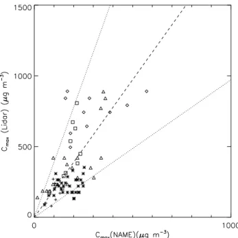
The peak concentrations from the lidar and from the cor-responding layers in the NAME simulations using the top emission profile are compared in Fig. 12. There is a reason-able correlation between the lidar and NAME for individual flights, which is similar to that found for the column mass loads (see Fig. 10). These correlations suggest that the
iden-tification of the observed ash layers with ash layers in the NAME simulations is justified. The ratios of lidar to NAME maximum concentrations are also listed in Table 1. They are larger than the corresponding ratios for the column integrated masses, consistent with the simulated layers being thicker than the observed ash layers (see Fig. 11). Comparison of the lidar and NAME estimates of the maximum concentra-tion (Fig. 12) indicates that, withαfestimated from the
col-umn integrated mass loads, the maximum concentrations are underestimated by a factor of∼2.
5 Discussion
This study has investigated how well the NAME model pre-dicted the structure of the ash clouds from the eruption of Ey-jafjallaj¨okull and the changes to the structure that occurred when the emission profiles were altered. Since it was not intended to produce the best simulations from NAME only simple emission profiles were considered.
For the 14, 16 and 17 May the ash features detected by the lidar could be readily associated with features in the NAME simulations, although there could be errors in the location of the simulated ash layers. Dacre et al. (2011) found timing errors of several hours in the predicted arrival of an ash layer over the southern UK at the start of the eruption in April. For these three days in May it was found that restricting the emission of ash to the upper part of the eruption plume gave the best comparison between NAME and the observations.
On the 4 and 5 May when the eruption intensity was low, although increasing, the situation is less clear. Arguably a uniform emission profile gives the best agreement between NAME and the observations. However, it is difficult for these days to accurately define the height of the eruption plume since it was frequently obscured from the radar at Keflavik (Arason et al., 2011). Dacre et al. (2011) and Devenish et al. (2011) show that short term variations in the height of the eruption plume can be detected in the ash cloud at long ranges. The use of the uniform emission profile may simply capture the effects of unresolved variations in the height of the eruption plume, even if the actual emission profile at any time has the ash source concentrated at the towards the top.
Fig. 11. Examples of concentration profiles, estimated from lidar extinction profiles on 14 May and simulated by NAME using the top emission profiles. The NAME profiles have been scaled by the distal fine ash fraction determined from the CIMLs. The small crosses are the estimates of concentration from the lidar extinction, the dashed curves show the fits to the lidar data and the solid curves are from NAME.
al. (2000) and the fine ash fraction estimated at the start of the eruption by Dacre et al. (2011).
The fine ash fraction derived in this study depends on the accuracy of the Mastin et al. (2009) relationship. The total mass of ash emitted into the atmosphere has been estimated to be 378±100 Tg based on sampling of the tephra blanket in Iceland (Gudmundsson et al , 2012). Using the height re-construction shown in Fig. 1 the mass erupted over the period of the eruption is 431 Tg, which is in reasonable agreement with the direct estimate. Stohl et al. (2011) and Kristiansen et al (2012) estimated the emissions of fine ash to be∼8 Tg, which with the direct estimate of the total erupted mass im-plies a fine ash fraction of∼2 %. This is in good agreement with the present estimate.
The ash clouds in NAME are significantly thicker than the observed ash layers, and this leads to a reduction in the max-imum concentration relative to the mean concentration. The increase in the thickness of the simulated ash clouds appears to occur close to the source, effectively spreading the emis-sions over a greater depth than that specified. Devenish et
al. (2011) show that for a period in April parametrizations intended to represent the effects of turbulence and meander-ing have a significant effect on the thickness of the simulated ash layers. The effective thickness of the emissions in the top emission profile is similar to that derived by Stohl et al. (2011) and Kristiansen et al (2012) using the inversion tech-nique. However, it is not clear to what extent their results, at least for the emissions derived from the NAME model, are affected by errors in the vertical structure of the simulated ash clouds found here.
Fig. 12. Comparison between maximum concentrations from the NAME simulations and estimated from the FAAM lidar. The NAME concentrations have been scaled by the distal fine ash frac-tion determined from the CIML. The symbols are the same as Fig. 10. The dashed line showsy=1.95x, the dotted lines have gradients that are twice and half those of the dashed line.
al., 2011; Kristiansen et al., 2012). Despite this the consis-tency of the results shows that using empirical relationships to estimate the emission source properties gives reasonable results, with the proviso that good observations of the height of the eruption plume are available.
6 Conclusions
Within the rather large uncertainties associated with the ob-servations the study suggests the following conclusions.
– The horizontal structure of the simulated ash clouds compares reasonably with the structure from the air-craft observations. However, there may be errors of or-der 100 km in the position of simulated ash clouds. – Generally having an elevated ash source gives the best
simulated ash clouds if information on the height of the eruption plume is available.
– Empirical relationships between the mass eruption rate and height of the eruption plume provide reasonable es-timates of concentrations when combined with an ap-propriate distal fine ash fraction.
– The comparisons suggest a distal fine ash fraction of 2–5 % for the Eyjafjallaj¨okull eruption, similar to
previ-ous estimates from other eruptions, and estimated from satellites for this eruption.
Overall this study shows that existing VATD models can be used to provide reasonable guidance on the structure and concentrations of ash in volcanic clouds to provide warnings to aviation in the event of an eruption.
Acknowledgements. The authors would like to thank Steve Sparks for helpful discussions on microphysical processes in volcanic clouds and for comments on the manuscript. We would also like to thank Helen Webster and Matthew Hort at the Met Office for useful feedback on the manuscript. Alan Grant was funded by a National Centre for Atmospheric Science (NCAS) national capability grant. Airborne data was obtained using the BAe-146-301 Atmospheric Research Aircraft (ARA) flown by Directflight Ltd and managed by the Facility for Airborne Atmospheric Measurements (FAAM), which is a joint entity of the Natural Environment Research Council (NERC) and the Met Office.
Edited by: G. Pappalardo
References
Arason, P., Petersen, G. N., and Bjornsson, H.: Observations of the altitude of the volcanic plume during the eruption of Eyjafjal-laj¨okull, April–May 2010, Earth Syst. Sci. Data, 3, 9–17, 2011, http://www.earth-syst-sci-data.net/3/9/2011/.
Ansmann, A.. Tesche, M., Gross, S., Freudenthaler, V., Seifert, P., Hiebsch, A., Schmidt, J., Wandinger, U., Mattis, I., Muller, D., and Wiegener, M.: The 16 April 2010 major volcanic ash plume over central Europe: EARLINET lidar and AERONET photome-ter observations at Leipzig and Munich Germany. Geophys. Res. Lett., 37, L13810, doi:10.1029/2010GL043809, 2010.
Bursik, M.: Effect of wind on the rise height of volcanic plumes, Geophys. Res. Lett., 18, 3621–3624, 2001.
Carey, S. and Sparks, S.: Quantitative models of the fallout and dis-persal of tephra from volcanic eruption columns, Bull. Volc., 48, 109–125, 1986.
Dacre, H. F., Grant, A. L. M., Hogan, R. J., Belcher, S. E., Thom-son, D. J., Devenish, B., Marenco, F., Hort, M., Haywood, J. M., Ansmann, A., Mattis, I., and Clarisse, L.: Evaluating the structure and magnitude of the ash plume during the initial phase of the 2010 Eyjafjallaj¨okull eruption using lidar observa-tions and NAME simulaobserva-tions, J. Geophys. Res., 116, D00U03, doi:10.1029/2011JD015608, 2011.
Dacre, H. F., Grant, A. L. M., Thomson, D. J., and Johnson, B. T.: Observations and model simulations of column integrated mass and grain size distribution in the Eyjafjallaj¨okull ash cloud, 12, 22587–22627,, doi:10.5194/acpd-12-22587-2012, 2012. Devenish, B. J., Thomson, D. J., Marenco, F., Leadbetter, S. J.,
Ricketts, H., and Dacre, H.: A study of the arrival over the United Kingdom in April 2010 of the Eyjafjallaj¨okull ash cloud using ground-based lidar and numerical simulations, Atmos. Environ., 48, 152–164, 2012.
measurements and inverse transport modeling, Atmos. Chem. Phys., 8, 3881–3897, doi:10.5194/acp-8-3881-2008, 2008. Flentje, H., Claude, H., Elste, T., Gilge, S., K¨ohler, U.,
Plass-D¨ulmer, C., Steinbrecht, W., Thomas, W., Werner, A., and Fricke, W.: The Eyjafjallaj¨okull eruption in April 2010 – detection of volcanic plume using in-situ measurements, ozone sondes and lidar-ceilometer profiles, Atmos. Chem. Phys., 10, 10085–10092, doi:10.5194/acp-10-10085-2010, 2010.
Folch, A., Costa, A., and Basart, S.: Validation of the FALL3D ash dispersion model using observations of the 2010 Eyafjallajokull volcanic ash clouds, accepted, Atmos. Environ., 48, 165–183, 2011.
Gudmundsson, M. T., Thordarson, T., H¨skuldsson, ´A., Laresen, G., Halld´or, B., Prata, F. J., Oddsson, B., Magn´usson, E., H¨gnad´ttir T., Petersen, G. N., Hayward, C. L., Stevenson, J. A., and J´onsd´ottir, I.: Ash generation and distribution from the April++May 2010 eruption of Eyjafallaj¨kull, Iceland., Sci. Rep., 2, 572, doi:10.1038/srep00572, 2012.
Heffter, J.L. and Stunder, B.J.B., 1993: Volcanic Ash Forecast Transport and Dispersion (VAFTAD) Model. Weather Forecast, 8, 534–541.
Johnson, B. T., Turnbull, K. F., Dorsey, J., Baran, A. K.,Ulanowski, Z., Hesse, E., Cotton, R., Brown, P. R. A., Burgess, R., Capes, G., Webster,H. N., Woolley, A. M., Rosenberg, P. D. and Haywood, J. M.: In-situ observations of volcanic ash clouds from the FAAM aircraft during the eruption of Eyjafjallaj¨okull in 2010, J. Geo-phys. Res., 117, D00U24, doi:10.1029/2011JD016760, 2011. Jones, A. R., Thomson, D. J., Hort, M., and Devenish, B.: The
U.K. Met Office’s next-generation atmospheric dispersion model NAME III: in: Air Pollution Modelling and its Application XVII, edited by: Borrego, C. and Norman, A.-L., (Proceedings of the 27 NATO/CCMS International Technical Meeting on Air Pollution Modelling and its Application), Springer, 580–589, 2007. Kristiansen, N. I., Stohl, A., Prata, A. J., Richter, A., Eckhardt, S.,
Seibert, P., Hoffmann, A., Ritter, C., Bitar, L., Duck, T. J., and Stebel, K.: Remote sensing and inverse transport modelling of the Kasatochi eruption sulphur dioxide cloud. J. Geophys. Res., 115, D00L16, doi:10.1029/2009/2009JD013286, 2010. Kristiansen, N.I., Stohl, A., Prata, A. J., Bukowiecki, N., Dacre, H.,
Eckhardt, S., Henne, S., Hort, M. C., Johnson, B. T., Marenco, F., Neninger, B., Reitebuch, O., Seibert, P., Thomson, D. J., Web-ster, H. N., and Weinzierl, B.: Performance assessment of a vol-canic ash transport model mini-ensemble used for inverse model-ing of the 2010 Eyjafjallaj¨okull eruption, J. Geophys. Res., 117, D00U11, doi:10.1029/2011JD016844, 2012.
Marenco, F., Johnson, B., Turnbull, K., Newman, S., Haywood, J., Webster H., and Ricketts, H.: Airborne lidar observations of the 2010 Eyjafjallaj¨okull volcanic ash plume, J. Geophys. Res., 116, D00U05, doi:10.1029/2011JD016396, 2011.
Mastin, L. G.: A user-friendly one-dimensional model for wet volcanic plumes, Geochem. Geophys. Geosyst., 8, Q03014, doi:10.1029/2006GC001455, 2007.
Mastin, L.G., Guffianti, M., Servranckx, R., Webley, P. W., Barsot-tie, S., Dean, K., Denlinger, R., Durant, A., Ewert, J. W., Gard-ner, C. A., Holliday, A. C., Neri, A., Rose, W. I., Schneider, D., Siebert, L., Stunder, B., Swanson, G., Tupper, A., Volentik, A., and Waythomas, C. F.: A multidisciplinary effort to assign re-alistic source parameters to model of volcanic ash-cloud trans-port and dispersion during eruptions. Journal of Volcanology and
Geothermal Research : Special Issue on Volcanic Ash Clouds, edited by: Mastin, L. and Webley, P., 186, 10–21, 2009. Petersen, G. N.: A short meteorological overview of the
Eyjafjallaj¨okull eruption 14 April–23 May 2010, Weather, doi:10.1002/wea.634, 2010.
Rauthe-Sch¨och, A., Weigelt, A., Hermann, M., Martinsson, B. G., Baker, A. K., Heue, K.-P., Brenninkmeijer, C. A. M., Zahn, A., Scharffe, D., Eckhardt, S., Stohl, A., and van Velthoven, P. F. J.: CARIBIC aircraft measurements of Eyjafjallaj¨okull volcanic clouds in April/May 2010, Atmos. Chem. Phys., 12, 879–902, doi:10.5194/acp-12-879-2012, 2012.
Rose, W. I., Bluth, G. J. S., and Ernst, G. G. J.: Integrating retrievals of volcanic cloud characteristics from satellite remote sensors: a summary, Phil. Trans. R. Soc. Lond. A, 358, 1585-1606, 2000. Schumann, U., Weinzierl, B., Reitebuch, O., Schlager, H., Minikin,
A., Forster, C., Baumann, R., Sailer, T., Graf, K., Mannstein, H., Voigt, C., Rahm, S., Simmet, R., Scheibe, M., Lichtenstern, M., Stock, P., R¨uba, H., Sch¨auble, D., Tafferner, A., Rautenhaus, M., Gerz, T., Ziereis, H., Krautstrunk, M., Mallaun, C., Gayet, J.-F., Lieke, K., Kandler, K., Ebert, M., Weinbruch, S., Stohl, A., Gasteiger, J., Groß, S., Freudenthaler, V., Wiegner, M., Ansmann, A., Tesche, M., Olafsson, H., and Sturm, K.: Airborne observa-tions of the Eyjafjalla volcano ash cloud over Europe during air space closure in April and May 2010, Atmos. Chem. Phys., 11, 2245–2279, doi:10.5194/acp-11-2245-2011, 2011.
Scollo, S., Folch, A., Coltelli, M. and Realmuto, V.J.: Three-dimensional volcanic aerosol dispersal: A comparison be-tween Multiangle Imaging Spectroradiaometer (MISR) data and numerical simulations. J. Geophys. Res., 115, D24210, doi:10.1029/2009JD013162, 2010.
Sparks, R. S., Bursik, J. M., Carey, S. N., Gilbert, J. S., Glaze, L. S., Siggurdsson, H. and Woods, A. W.: Volcanic Plumes, John Wiley and Sons, Chichester, UK, 1997.
Stohl, A., Prata, A. J., Eckhardt, S., Clarisse, L., Durant, A., Henne, S., Kristiansen, N. I., Minikin, A., Schumann, U., Seibert, P., Stebel, K., Thomas, H. E., Thorsteinsson, T., Tørseth, K., and Weinzierl, B.: Determination of time- and height-resolved vol-canic ash emissions and their use for quantitative ash disper-sion modeling: the 2010 Eyjafjallaj¨okull eruption, Atmos. Chem. Phys., 11, 4333–4351, doi:10.5194/acp-11-4333-2011, 2011. Thomas, H. E. and Prata, A. J.: Sulphur dioxide as a volcanic
ash proxy during the April–May 2010 eruption of the Eyjafjal-laj¨okull volcano, Iceland, Atmos. Chem. Phys., doi:10.5194/acp-11-6871-2011, 2011.
Turnbull, K., Johnson, B., Marenco, F. Haywood, J., Minikin, A., Weinzierl, B., Schlager, H., Schumann, U., Leadbetter, S., and Wooley, A.: A case study of observations of volcanic ash from the Eyjafjallaj¨okull eruption: 1. In situ airborne observations. J. Geophys. Res., 117, D00U12, doi:10.1029/2011JD016688, 2012.
Webley, P. W., Atkinson, D., Collins, R. L., Dean, K., Fochesatto, J., Sassen, K., Cahill, C. F., Prata, A., Flynn, C. J., and Mizu-tani, K.: Predicting and validating the tracking of a volcanic ash cloud during the 2006 eruption of Mt Augustine Volcano, B. Am. Meteor. Soc., 89, 1647–1658, 2008.
Alaska, J. Volcanol. Geotherm. Res., 186, 108–119, 2009. Webster, H. N., Thomson, D. J., Johnson, B. T., Heard, I. P. C.,
Turn-bull, K. F., Marenco, F., Kristiansen, N. I., Dorsey, J. R., Minikin, A., Weinzierl, B., Schumann, U., Sparks, S. S. J., Loughlin S. C., Hort, M., Leadbetter, S. J., Devenish, B., Manning, A. J., Witham, C., Haywood, J. M., and Golding, B.: Operational pre-diction of ash concentrations in the distal volcanic cloud from the 2010 Eyjafjallajokull eruption, J. Geophys. Res., 117, D00U08, doi:10.1029/2011JD016790, 2012.