www.hydrol-earth-syst-sci.net/16/3959/2012/ doi:10.5194/hess-16-3959-2012
© Author(s) 2012. CC Attribution 3.0 License.
Earth System
Sciences
Modelling shallow landslide susceptibility by means of a subsurface
flow path connectivity index and estimates of soil depth spatial
distribution
C. Lanni1, M. Borga2, R. Rigon1, and P. Tarolli2
1Department of Civil and Environmental Engineering, University of Trento, Trento, Italy 2Dipartimento Territorio e Sistemi Agro-Forestali, Universit`a di Padova, Padova, Italy Correspondence to:C. Lanni ([email protected])
Received: 8 March 2012 – Published in Hydrol. Earth Syst. Sci. Discuss.: 28 March 2012 Revised: 28 August 2012 – Accepted: 4 September 2012 – Published: 2 November 2012
Abstract. Topographic index-based hydrological models have gained wide use to describe the hydrological control on the triggering of rainfall-induced shallow landslides at the catchment scale. A common assumption in these models is that a spatially continuous water table occurs simultaneously across the catchment. However, during a rainfall event iso-lated patches of subsurface saturation form above an imped-ing layer and their hydrological connectivity is a necessary condition for lateral flow initiation at a point on the hillslope. Here, a new hydrological model is presented, which al-lows us to account for the concept of hydrological connec-tivity while keeping the simplicity of the topographic index approach. A dynamic topographic index is used to describe the transient lateral flow that is established at a hillslope el-ement when the rainfall amount exceeds a threshold value allowing for (a) development of a perched water table above an impeding layer, and (b) hydrological connectivity between the hillslope element and its own upslope contributing area. A spatially variable soil depth is the main control of hydro-logical connectivity in the model. The hydrohydro-logical model is coupled with the infinite slope stability model and with a scaling model for the rainfall frequency–duration relation-ship to determine the return period of the critical rainfall needed to cause instability on three catchments located in the Italian Alps, where a survey of soil depth spatial distribution is available. The model is compared with a quasi-dynamic model in which the dynamic nature of the hydrological con-nectivity is neglected. The results show a better performance of the new model in predicting observed shallow landslides, implying that soil depth spatial variability and connectivity bear a significant control on shallow landsliding.
1 Introduction
Effective management of the hazard associated with shal-low landsliding requires information on both the location of potentially unstable hillslopes and the conditions that cause slope instability. The need for spatial assessment of land-slide hazard, along with the widespread use of Geographical Information Systems (GISs), has led to the proliferation of mathematical, GIS-based models (e.g. Montgomery and Di-etrich, 1994; Pack et al., 1998; Borga et al., 2002a; Tarolli and Tarboton, 2006; Baum et al., 2008) that can be applied over broad regions to assist forecasting, planning, and risk mitigation. Such models couple a hydrologic model, for the analysis of the pore-water pressure regime, with an infinite slope stability model, for the computation of the factor of safety (i.e. the ratio of retaining to driving forces within the slope) at each point of a landscape.
expressed as a function of TWI. Borga et al. (2002b) relaxed the hydrological steady-state assumption used in SHAL-STAB by using a modified version of the quasi-dynamic wet-ness index developed by Barling et al. (1994). This model, called Quasi-Dynamic Shallow Landsliding Model – QD-SLaM, permits us to describe the transient nature of lateral subsurface flow (Grayson et al., 1997).
However, research in the last decade has shown that the establishment of hydrological connectivity (the condition by which disparate regions on the hillslope are linked via sub-surface water flow, Stieglitz et al., 2003) is a necessary condition for lateral subsurface flow to occur at a point (e.g. Spence and Woo, 2003; Buttle et al., 2004; Graham et al., 2010; Spence, 2010). Lack of or only intermittent connectivity of subsurface flow systems invalidates the as-sumptions built into the TWI theory (i.e. the variable – and continuum – contributing area concept originally proposed by Hewlett and Hibbert, 1967). Both field (e.g. Freer et al., 2002; Tromp van Meerveld and McDonnell, 2006) and nu-merical (e.g. Hopp and McDonnell, 2009; Lanni et al., 2012) studies have shown that subsurface topography (and there-fore soil-depth variability) has a strong impact in controlling the connectivity of saturated zones at the soil–bedrock inter-face, and in determining timing and position of shallow land-slide initiation (Lanni et al., 2012). However, despite these evidences, most shallow landslide models do not include a connectivity component for subsurface flow modelling.
Here, we propose a new Connectivity Index-based Shal-low LAndslide Model (CI-SLAM) that includes the concept of hydrological connectivity in the description of the subsur-face flow processes while keeping the simplicity of the topo-graphic index approach needed to conduct large scale analy-sis. In our model framework, hydrological connectivity is re-lated to the spatial variability of soil depth across the inves-tigated catchments and the initial soil moisture conditions. Vertical rainwater infiltration into unsaturated soil is simu-lated by using the concept of drainable porosity (i.e. the vol-ume of stored soil-water removed/added per unit area per unit decline/growth of water table level; Hilberts et al., 2005; Cor-dano and Rigon, 2008). This allows simulation of pore-water pressure dynamics under the assumption of quasi-steady state hydraulic equilibrium and to estimate the time for devel-opment of saturated conditions at the soil/bedrock interface. The model incorporates the computation of a characteristic time for describing the connection of these “patches” of sat-uration. Specifically, it is assumed that an element (x, y) in a hillslope connects (hydrologically) with its own upslope con-tributing areaA(x, y)when the water table forms a continu-ous surface throughoutA(x, y). Once hydrological connec-tivity is established, the dynamic topographic index devel-oped by Lanni et al. (2011) is used to describe the transient subsurface flow converging to the element in (x, y).
The hydrological module is then coupled with the infinite slope stability equation to derive CI-SLAM, a shallow land-slide model which is able to (a) account for the (positive)
effect of the unsaturated zone storage on slope stability, and (b) reproduce pre-storm unsaturated soil conditions. This im-plicitly helps reducing the fraction of catchment area which is categorized as unconditionally unstable (i.e. failing even under dry soil moisture conditions), improving the confi-dence in model results (Keijsers et al., 2011).
Model testing is carried out in three study sites located in the central Italian Alps. In this area, shallow landslides are generally triggered by local, convective storms during the summer and early fall seasons. Moreover, accurate field surveys provide a description of hydraulic and geotechnical properties of soils, and a detailed representation of soil depth variation as a function of local slope is reported. An inventory of shallow landslides is also available. Finally, the proposed shallow landslide model is compared with a quasi-dynamic model (QDSLaM) in order to gain insight on the potential improvement brought by the new modelling framework.
2 The modelling framework
2.1 The hydrological model
Figure 1 schematizes the hydrological model developed here. During a rainfall event the generation of lateral flow is pre-ceded by the development of a positive pressure head (i.e. perched water table) at the soil-bedrock interface. Several researchers (McNamara et al., 2005; Rahardjo et al., 2005; D’Odorico et al., 2005) have shown that vertical flow in the unsaturated soil zone is reduced when the infiltration front meets a less permeable layer (for example, the bedrock layer). Under this condition, the infiltrating rainwater col-lects at the less permeable soil layer, inducing rapid increases of pore-water pressure and unsaturated hydraulic conduc-tivity (according to the relationship between matric suction head and unsaturated hydraulic conductivity). As a result, a perched water table will form on the surface of the low-conductive layer, and a subsurface flow will move laterally along the upper surface of this layer (e.g. Weyman, 1973; Weiler et al., 2005). Moreover, in the model it is assumed that a generic hillslope element (x, y) receives flow from the related upslope catchment area A(x, y)only when isolated patches of transient saturation become connected with ele-ment (x, y) (Fig. 2).
In the model, unsaturated soil conditions through the whole soil profile (i.e. positive suction head or negative pres-sure head) are used to initialize our model (step 1 in Fig. 1). For each hillslope element (x, y), the timetwt(x, y)needed
to build up a perched zone of positive pore pressure at the soil–bedrock interface is computed by using the following expression (step 2 in Fig. 1):
twt(x, y) =
Vwt(x, y)−V0(x, y)
I , (1)
whereV0[L] is the initial storage of soil moisture through the
Fig. 1.A flow chart depicting the coupled saturated/unsaturated hydrological model developed in this study.
Fig. 2.The concept of hydrological connectivity. Lateral subsurface flow occurs at point (x, y) when this becomes hydrologically con-nected with its own upslope contributing areaA(x, y).
storage of soil moisture needed to produce a perched water table (i.e. zero-pressure head) at the soil–bedrock interface (Fig. 3); andI [LT−1] is the rainfall intensity assumed to be
uniform in space and time. Computation ofV0 andVwt
re-quire the use of a relationship between soil moisture content θ[−] and suction headψ[L], and a relationship betweenψ and the vertical coordinate (positive upward)z[L] (Fig. 3).
By using the assumption that the suction head profileψ (z) changes from one steady-state situation to another over time,
Fig. 3.θi(z)and ψi(z)are, respectively, the initial water content and the initial suction head vertical profiles.θwt(z)andψwt(z) rep-resents the linear water content and suction head vertical profiles associated with zero-suction head at the soil–bedrock interface.
the relation between ψ [L] and z [L] is that of hydraulic equilibrium:
ψ =ψ (z =0)+z=ψb+z, (2)
whereψb=ψ (z=0)is the suction head at the soil–bedrock
is rapid. The constitutive relationship betweenθandψused in this study is the van Genuchten function (van Genuchten, 1980):
θ (ψ )=θr+(θsat−θr)1+(αψ )n−m (3)
withθsat[−] = saturated water content;θr[−] = residual
wa-ter content;α[L−1] = parameter that depends approximately on the air-entry (or air-occlusion) suction; andn[−] andm [−] = van Genuchten parameters. Combining Eqs. (2) and (3) we obtain:
θ (ψ )=θr+(θsat−θr)1+(α (ψb+z))n−m. (4)
Based on Troch (1992), the following relationship between the parametersmandnis used in the model:
m=1+n1, (5)
The storage of soil moisture through the soil profileV is ob-tained by integrating Eq. (4) from the bedrock to the ground surface:
V =
z=L
Z
z=0
θ (z)dz=θr·L+(θsat−θr)
(L+ψb) 1+(α (L+ψb))n
−1n
−ψb 1+(αψb)n −1n
.(6)
whereL [L] is the soil depth measured along the vertical. Vwt can be obtained by setting a zero-pressure head at the
soil–bedrock interface (ψb= 0):
Vwt =θr·L+(θsat−θr)·L· 1+(αL)n− 1
n. (7)
The suction head value at the soil–bedrock interface at a generic time t < twt(x, y) (i.e. before development of a
perched water table), ψbt, can be calculated by using the
concept of drainable porosityf [−] proposed by Hilberts et al. (2005):
f = dV dψb =
(θsat−θr)·
1+(α (L+ψb))n−1− 1 n
− 1+(αψb)n−1− 1 n
. (8)
By using Eq. (8), we can derive an expression for dψb/dt,
useful for estimating the suction head at the soil–bedrock in-terface at a generic timet,ψbt (step 5a in Fig. 1):
dψb dt =
I f
implies
⇒ ψbt=ψbt−1 (9)
+ I
(θsat−θr)·
1+(α (L+ψb))n−1−n1
− 1+(αψb)n−1−1n
1t.
where1tis the temporal integration time. Fort≥twt(x, y),
the generic hillslope element (x, y) exhibits a perched water table at the soil–bedrock interface.
However, this does not guarantee the hydrological connec-tivity between element (x, y) and its related upslope con-tributing area A(x, y). In fact, due to the heterogeneity of initial soil moisture and soil depth, isolated patches of sat-uration which do not necessarily connect with point (x, y) may have developed insideA(x, y). We assume that lateral subsurface flow affects the local soil-water storage of point (x, y) when the water table timetwtindicates continuous
sat-uration throughA(x, y). Thus, each point (x, y) has two wa-ter table characwa-teristic times: (1)twt, which indicates the local
time for the development of a perched water table; and (2) a connectivity timetwtup– given by the maximum value oftwtin
A(x, y)– which indicates the time required by element (x, y) to become hydrologically connected withA(x, y). Therefore, a generic hillslope element (x, y) receives flow from its own upslope contributing area starting fromt=twtup(x, y)(steps 3 and 4b in Fig. 1). Details on the formulation of the connec-tivity timetwtupare given in Appendix A.
The value of the lateral flow rate at element (x, y) is then calculated by using the upslope contributing areaA(x, y)as a surrogate for lateral flow (Borga et al., 2002b). In particular, we use the method proposed by Lanni et al. (2011) to de-scribe the variable upslope contributing area which changes linearly with time:
At(x, y)=
t−twtup(x, y) τc(x, y)−twtup(x, y)
A(x, y)
for twtup(x, y) < t ≤ τc(x, y)≤d (10a)
At(x, y)=A(x, y) for τc(x, y) ≤t ≤d (10b)
At(x, y)=max
0, A(x, y)
1+ d−t
τc(x, y)−twtup(x, y)
for t ≥d ≥ τc(x, y)≥ twtop(x, y) (10c)
At(x, y)=max
0, A(x, y)
1+ 2d−t
up
wt(x, y)−t τc(x, y)−twtup(x, y)
for t ≥d ≥ twtup(x, y) if τc(x, y) > d (10d) where At(x, y) [L2] and A(x, y) [L2] are the time
vari-able upslope contributing area and the steady state upslope contributing area extending to the divide, respectively; t [T] = time;d [T] = rainfall duration;τc(x, y)is given by the
combination oftwtup(x, y)and the timeτc′(x, y)required to the lateral flow to reach point (x, y) from the most hydrologically remote location in the corresponding drainage areaA(x, y):
τc(x, y)=τc′(x, y)+t up
wt(x, y) (11)
The value ofτc′(x, y)is computed based on the method de-scribed in Lanni et al. (2011).
t≥twtup(x, y),hbt(x, y), is given by (step 6b2 in Fig. 1):
hbt(x, y)= −ψbt(x, y)
=min
I Ksat(x, y) ·
At(x, y)
b(x, y)·sin[β(x, y)], L(x, y)
, (12) whereβis the local ground inclination,Ksat(x, y)[L T−1] is
the saturated hydraulic conductivity andAt/b[L] is the time
variable contributing area at timetper unit contour length. 2.2 The coupled hydrological slope stability model,
CI-SLAM
For hillslopes it is common to define the safety factor as the ratio between maximum retaining forces,Fr, and driving
forces,Fd:
FS= Fr
Fd
. (13)
The slope is stable for FS>1, while slope failure occurs when the critical state FS = 1 (such thatFr=Fd) is achieved.
Lu and Likos (2006) derived a formulation to compute the factor of safety of an infinite slope model that accounts for saturated/unsaturated zones. If the failure surface is located at the soil–bedrock interface, then the Lu and Likos’ factor of safety can be written as:
FS= 2·c
′
γ ·L·sin[2β]+ tanϕ′
tanβ
+Se(ψb)
γw
γ ψb
L (tanβ +cotβ)·tanϕ
′
for ψb >0(hb <0) (14a)
FS= 2·c
′
γ ·L·sin[2β]+
tanϕ′
tanβ +
γw
γ
ψb
L (tanβ+cotβ)·tanϕ
′
for ψb ≤0(hb≥0) (14b)
withc′[FL−2] = effective soil cohesion;ϕ′[◦] = effective soil
frictional angle;γwandγ[FL−3] = volumetric unit weight of
water and soil, respectively; andSe[−] = relative saturation
degree. Equations (14a, b) allow the (positive) role played by suction head on the hillslope stability to be taken into ac-count. In this work, locations that are neither unconditionally unstable or unconditionally stable (i.e. locations that are sta-ble when saturated) will be called conditionally unstasta-ble as proposed in the pioneering work of Montgomery and Diet-rich (1994).
By coupling the hydrological model (Eqs. 9 and 12) with the slope stability model (Eqs. 14a, b) the factor of safety for conditionally unstable locations (x, y) at a generic timet reads:
FSt(x, y) =
2·c′(x, y)
γ ·L·sin [2β(x, y)] +
tanϕ′(x, y)
tanβ(x, y)
+Se ψbt(x, y)
γw(x, y)
γ (x, y)
ψbt(x, y)
L(x, y) (tanβ(x, y)+cotβ(x, y))·tanϕ′(x, y) forψbt(x, y) >0 hbt(x, y) <0
(15a) FSt(x, y) =
2·c′(x, y) γ ·L·sin[2β(x, y)] +
tanϕ′(x, y) tanβ(x, y)
+γγ (x, y)w(x, y) K I
sat(x, y)·L(x, y)
At(x, y)
b(x, y)·sinβ(x, y)
(tanβ(x, y)+cotβ(x, y))·tanϕ′(x, y) for ψbt(x, y) ≤0 hbt(x, y)≥ 0
. (15b)
2.3 Intensity–duration–frequency relationship for extreme storms
The variability of rainfall intensity with rainfall duration for a specified frequency level is often represented by the intensity–duration–frequency (IDF) relationship proposed by Koutsoyiannis et al. (1998):
IF(d)=ςF ·dmF−1 (16)
withIF(d)= rainfall intensity that can be exceeded with a
probability of 1−F.ςF andmF are parameters estimated by
least squares regression ofIF(d)against rainfall durationd. It
has been shown (Burlando and Rosso, 1996) that a Gumbel simple scaling model describes well the distribution of an-nual maximum series of rainfall in the Central Italian Alps. Based on this model, the rainfall intensityIF(d)can be
de-termined as: IF(d)=ς1
"
1− CV √
6
π ε+yTR
#
·dm−1 (17) withε= Euler’s constant (∼0.5772).ς1andmcan be
esti-mated by linear regression of expectations of rainfall depth against duration, after log transformation, whereas the value of the coefficient of variation (CV) can be obtained as the average of coefficients of variation computed for the differ-ent durations, in the range of durations for which the scaling property holds.yTRis given by:
yTR =ln
ln
T
R
TR−1
,
(18) whereTR[T] is the return period. By combining Eqs. (17)
and (18),TRcan be written as a function of rainfall intensity
and duration:
TR=
exphexph π
CV√6
1−ς1IdFm(d)−1
−εii exphexph π
CV√6
1−ς1IdFm(d)−1
−εii−1
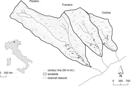
Fig. 4.Study catchments. The map shows the location of the three catchments, and the landslide distribution.
3 Study sites and the analysis of soil depth variability
The study area is represented by three small catchments located in the central Italian Alps: Pizzano, Fraviano, and Cortina (Fig. 4), with sizes of 4.43, 2.00 and 1.03 km2, respectively, and overall surface of 7.46 km2. A 10 m-resolution DEM, derived from a 1:10 000 scale contour map, is available for the study area. Elevations (E) range from 1250 to 2830 m a.s.l., with an average value of 1999 m a.s.l. Pizzano is characterized by higher elevations, whereas Cortina is located at lower altitudes, with Fraviano in in-termediate position. Cortina and Fraviano have similar slope distribution, with mean slopes of 27.5◦and 28◦, respectively. Pizzano is steeper, with a slope of 30.4◦. The morphology of the catchments shows two different structures: a flatter area in the upper portions of the basins, and a narrow, steeper river course in the downstream portions. The vegetation dis-tribution is controlled by the tree-line altitude, with Cortina exhibiting a larger portion of forest stands (74.2 %) (mainly conifers) than Fraviano and Pizzano, where forest covers a lower percentage of the basins (around 55 %). The remain-ing land cover is represented by grassland (8.2 % for Cortina and 24 % for Fraviano and Pizzano) and bedrock outcrops.
Most of the shallow landslides analyzed in this work were triggered during the falls of 2000 and 2002 as a result of relatively short duration storms. The landslide inventory de-scribed in this work is part of a more comprehensive archive of shallow landslides which has been described in other pa-pers as well (Borga et al., 1998, 2002a,b, 2004; Tarolli et al., 2008, 2011) and executed with a common surveying method-ology. The landslides were surveyed during the fall of 2005 and their spatial distribution is reported in Fig. 4, where only the initiation areas are shown. Most of the landslides
are found in the lower portion of the basins, where the ter-rain is steeper and the soil may be deep enough to trigger slope instability. During the survey, the shallow landslides which were evidently induced by forest roads were marked and identified as such and excluded from the model analysis. 3.1 Soil depth survey and the relationship with the
local slope
Roering et al. (1999) supported the idea that soil production follows a non-linear equation and, therefore, modified the de-pendence of soil depth relationships. However, the various modelling approaches for predicting soil depth over land-scapes, described above, showed only partial success (Tesfa et al., 2009).
In contrast to the process-based approaches, a number of studies have applied statistical methods to identify relation-ships between soil depth and landscape topographic variables (e.g. slope, wetness index, plan curvature, distance from hill-top, or total contributing area) (e.g. Gessler et al., 1995; Tesfa et al., 2009; Catani et al., 2010). Some of these works re-ported good predictive capabilities for these statistical rela-tionships. For instance, Tesfa et al. (2009) report that their statistical models were able to explain about 50 % of the mea-sured soil depth variability in an out-of-sample test. This is an important result, given the complex local variation of soil depth.
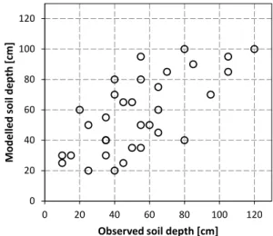
For the purpose of this work, we use a statistical approach for the estimation of the spatial distribution of soil depth over the study catchments. This is based on the availabil-ity of a rather dense sample of soil depth measurements. During the fieldwork, conducted in the fall of 2005, 410 di-rect point measurements of soil depth were made. Survey lo-cations were chosen to represent the range of topographic variation in the areas of model application. Measurements were carried out by driving a 150 cm long, 1.27 cm diam-eter, sharpened, copper-coated steel rod graduated at 5 cm intervals vertically into the ground until refusal. The advan-tage of the depth to refusal method is that it is a direct and simple measurement of soil depth. A disadvantage is that the measurement is biased to underestimating the actual depth to bedrock, since there is uncertainty as to what actually causes refusal. Each point measurement is represented by the aver-age of the measures from two or three replicates taken very close each other (at less than 0.5 m distance) (three replicates were taken when the difference between the first two was more than 20 cm). In order to represent soil depth over the extent of grid-size topographic elements, the survey was car-ried out by taking five point measures 2–3 m apart over a 5 m size grid. A “grid-size” soil depth observation was ob-tained by taking the average over the five point measures. This permitted us to obtain 82 grid-size observations, which were divided into two subsets: the first (49 grid-size observa-tions) was used to identify and calibrate the statistical model, the second (33 grid-size observations) was used to perform a validation.
The field measurements allowed us to derive the following relationship between soil depthLand local slope tanβ: L(x, y)=1.01−0.85 tanβ(x, y). (20) Equation (20) is limited to local slope less than 45◦(below 2000 m a.s.l.) and 40◦(above 2000 m a.s.l.). In fact, locations with local slope angle larger than these threshold angles are generally characterized by rocky outcrops or very shallow
0 20 40 60 80 100 120
0 20 40 60 80 100 120
M
od
e
ll
e
d
so
il
d
e
p
th
[
cm]
Observed soil depth [cm]
Fig. 5.Validation of the soil depth–local slope model: modelled ver-sus observed soil depth over 33 grid-size observations.
soil thickness and discontinuous soil coverage. The eleva-tion of 2000 m a.s.l. defines a threshold in soil pedological properties (as reported also by Aberegg et al., 2009). The analysis of the soil type distribution showed that Episkeletic Podzols and Dystri-Chromic Cambisols predominantly ap-pear on slopes between 1400 to 1900 m a.s.l. Enti-Umbric Podzols are characteristic for southern exposures at altitudes higher than 2000 m a.s.l.
Other topographic variables, such as plan curvature and specific catchment area, and land cover attributes showed no statistically significant relationship with soil depth. The rela-tionship between soil depth and slope identified for the study watersheds is consistent with findings reported in the litera-ture (Saulnier et al., 1997; Tesfa et al., 2009).
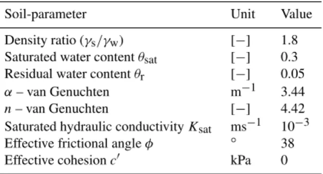
Table 1.Hydraulic and mechanical soil parameters relative to the three investigated catchments.
Soil-parameter Unit Value
Density ratio (γs/γw) [−] 1.8
Saturated water contentθsat [−] 0.3
Residual water contentθr [−] 0.05
α– van Genuchten m−1 3.44
n– van Genuchten [−] 4.42
Saturated hydraulic conductivityKsat ms−1 10−3
Effective frictional angleφ ◦ 38
Effective cohesionc′ kPa 0
3.2 Model application
CI-SLAM has been applied on the study catchments by us-ing the hydraulic and mechanical soil parameters reported in Table 1, identified based on a field survey carried out during the summer season 2005. The soil properties are assumed to be the same for all the three catchments. Based on ob-servations on the erosion crowns and along the forest roads, the survey revealed that the trees in this area are character-ized by shallow root systems that spread laterally with small vertical sinker roots that penetrate deeper into the soil. Ow-ing to these observations, we decide not to consider the root strength contribution into the shallow landslide stability anal-ysis. Since the factor of safety calculated by the infinite slope stability equation is fairly insensitive to the values of tree surcharge (Borga et al., 2002a), we omitted considering this factor too.
The soil moisture initial conditions were assumed to rep-resent average climatic conditions based on estimated evapo-transpiration fluxes and inter-storm duration statistics which are typical of the seasons where shallow landslides were recorded (summer season and first half of the fall season). These unsaturated soil moisture conditions correspond to considerable cohesion which is due to capillarity, as concep-tualized in the generalized principle of effective stress (Lu and Godt, 2008; Godt et al., 2009).
We used the procedure reported by Borga et al. (2005) to estimate the following scaling parameters of the IDF rela-tionship (Eq. 18): CV = 0.42,m= 0.48,ς1= 13.7 mm h1−0.48.
These parameters are kept spatially uniform across the three catchments.
The model was not implemented on areas likely char-acterized by bedrock outcrops, i.e. on topographic ele-ments characterized by slope exceeding either 45◦(for ele-vation<2000 m a.s.l.) or 40◦(for elevation≥2000 m a.s.l.). These areas amount to low percentages on Cortina and Fra-viano (with 0.7 % and 1 % of catchment area, respectively), whereas they are much more considerable on the steeper Piz-zano catchment, where they amount to 11.7 %.
Two general procedures may be considered for shal-low landslide model application: diagnostic and predictive (Rosso et al., 2006). With the first procedure, terrain stability is simulated for a given temporal pattern of rainfall intensity and for given initial soil moisture conditions. This allows ex-ploration of the pattern of instability generated by specific storms and could be used to make real-time forecast of shal-low landslides. In the predictive mode, the shal-lowest return pe-riod of the critical rainfall is computed for each condition-ally unstable cell in the landscape. This procedure is well suited for generating maps of shallow landsliding suscepti-bility, and can be specifically adapted to assess CI-SLAM’s capability of predicting shallow landslides which are gener-ated by multiple storms with different storm depth and inten-sities. The predictive procedure is adopted in this work based on the following steps. First, the critical durationdcof
rain-fall which generates instability (i.e. FS = 1) is computed for a range of constant rainfall intensitiesI (ranging from 5 to 60 mm h−1at a 5 mm h−1step) which are kept uniform both
in time and in space. Then, the return periodTris computed
for each considered (I, dc) pair by using Eq. (19). Finally,
the lowest return period for each conditionally stable loca-tion is selected. The map of the return period of the critical rainfall will provide a representation of the susceptibility to shallow landsliding across the landscape.
4 Results and comparison with QDSLaM
By using the predictive procedure discussed in the previous paragraph, we derived the shallow landslide susceptibility map of Fig. 6, where the surveyed landslides are also re-ported. The criterion of shallow landslide susceptibility is based on the return period of the critical rainfall; higher re-turn period values represent medium (TR= 30–100 yr) and
low (TR>100 yr) shallow landslide propensity, and lower
re-turn period values represent high (TR= 10–30 yr) and very
high (TR<10 yr) shallow landslide propensity. A “very low”
level of shallow landslide susceptibility is assigned to uncon-ditionally stable points (i.e. locations that are stable when completely saturated).
The landslide susceptibility map indicates that the catch-ments can be subdivided into two geomorphological units. Topographic elements with very high shallow landsliding susceptibility (TR<10 yr) are reported only in the lower
por-tion of the three catchments, where also surveyed shallow landslides are reported. Conversely, areas characterized as “unconditionally stable” or with very low landsliding suscep-tibility (TR>100 yr) are found mostly in the upper portion of
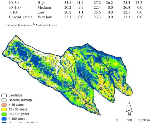
Table 2.Percentages of catchment area (C) and observed landslide area (L) in each range of critical rainfall frequency (i.e. return periodTR) for CI-SLAM.
TR Susceptibility Pizzano Fraviano Cortina
level
Ca Lb Ca Lb Ca Lb
Years Category % % % % % %
0–10 Very high 1.8 51.6 2.5 63.8 3.9 24.3
10–30 High 34.1 41.4 27.2 36.2 24.3 75.7
30–100 Medium 20.2 5.9 22.4 0.0 26.4 0.0
>100 Low 20.2 1.1 25.6 0.0 22.1 0.0
Uncond. stable Very low 23.7 0.0 23.3 0.0 23.3 0.0
aC= catchment area;bL= landslide area
triggering (i.e., FS≤1) and associated levels of lands
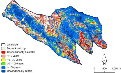
Fig. 6.Patterns of return periodTR(years) of the critical rainfalls for shallow landslide triggering (i.e. FS≤1) and associated levels of landslide susceptibility obtained by means of CI-SLAM.
critical rainfall ranges with the corresponding fraction of the landslide area (Table 2). Good model performances are ex-pected when a large percentage of observed landslides and a small percentage of catchment area occur for low values of return time. For example, this is the case for the Pizzano basin where the percentage of catchment area with TR in
the range of 0–10 yr is equal to 1.8 % (34.1 % in the range of 10–30 yr), while the corresponding fraction of observed landslide area is equal to 51.6 % (41.4 % in the range of 10– 30 yr). On the other hand, the percentage of landslide area withTR>100 yr is only 1.1 % versus 43.9 % of the
catch-ment area (including the locations classified as uncondition-ally stable). Therefore, CI-SLAM is able to correctly classify with a high or very high levels of shallow landslide suscepti-bility most of the observed landslide areas. This is confirmed by the results for the Cortina and the Fraviano catchments, with this last one showing the best model predictions (63.8 %
of landslide area falling in the 2.5 % of catchment area with TR≤10 yr).
Our results suggest that model predictions capture a high percentage of observed landslides at the expense of some overprediction of slope instability. However, one should note that overprediction of landsliding susceptibility has been ob-served in other applications of topographic index-based shal-low landsliding models (e.g. Dietrich et al., 2001) and may be due to a number of reasons, including: (i) inaccurate to-pographic data, (ii) legacy effects of previous landslides, and (iii) limitation of the landslide surveys.
Comparison with QDSLaM
triggering (i.e., FS≤1) and associated levels of landslide susceptibility obtained by means
Fig. 7.Patterns of return periodTR(years) of the critical rainfalls for shallow landslide triggering (i.e. FS≤1) and associated levels of landslide susceptibility obtained by means of QDSLaM.
Table 3.Percentages of catchment area (C) and observed landslide area (L) in each range of critical rainfall frequency (i.e. return periodTR) for QDSLaM.
Susceptibility Pizzano Fraviano Cortina
TR level Ca Lb Ca Lb Ca Lb
Years Category % % % % % %
Uncond Unstable 9.9 60.2 7.7 77.7 8.5 56.8
0–10 Very high 20.3 26.9 16.1 18.5 13.5 39.2
10–30 High 7.8 0.0 5.6 1.5 5.8 4.0
30–100 Medium 6.0 9.7 5.9 2.3 6.7 0.0
>100 Low 42.9 3.2 53.5 0.0 54.7 0.0
Uncond. stable Very low 13.1 0.0 11.2 0.0 10.8 0.0
aC= catchment area;bL= landslide area
high slope failure hazard) of CI-SLAM with that of the quasi-dynamic model QDSLaM (Borga et al., 2002b).
QDSLaM is based on coupling a hydrological model to a limit-equilibrium slope stability model to calculate the critical rainfall necessary to trigger slope instability at any point in the landscape. The hydrological model assumes that flow infiltrates to a lower conductivity layer and fol-lows topographically-determined flow paths to map the spa-tial pattern of soil saturation based on analysis of a “quasi-dynamic” wetness index. With respect to the model pro-posed in this paper, QDSLaM does not consider the follow-ing aspects: (i) vertical rainwater infiltration into unsaturated soil; (ii) analysis of the connectivity to compute the quasi-dynamic wetness index; and (iii) soil depth variability. All re-maining aspects of the modelling framework are described in a consistent way by the two models. Both models have been applied to the three catchments by using the same parameters
set. A map of shallow landsliding susceptibility obtained by using QDSLaM is reported in Fig. 7, whereas Table 3 reports the corresponding percentages of slope-stability categories in terms of catchment area and observed landslide area in each range of critical rainfall frequency (i.e. return periodTR).
as by other traditional landslide models, e.g. Montgomery and Dietrich, 1994; Wu and Sidle, 1995; Pack et al., 1998, among others), which does not account for the role of nega-tive pressure head on soil shear strength.
We also carried out a comparison of the areas which are considered as conditionally unstable by both models. The procedure consists of comparing the proportions of catch-ment area which fall beneath various return time levels to the corresponding fraction of the landslide area. To compare the two models, theTRvalues are set so that the same percentage
of terrain elements falls beneath the values. The two sets of unstable regions, resulting from the application of the mod-els, are partially overlapping but are not the same. Then the percentage of observed landslide area within each unstable region is computed. The model with the higher percentage provides a better prediction of landslide hazard. This assess-ment may be repeated for variousTRvalues, obtaining two
empirical distribution functionsFB(TR)andFL(TR),defined
for the terrain elements and for the observed landslide cells, respectively. FB(TR) and FL(TR) represent the fraction of
catchment area and of landslide area, respectively, charac-terized by return time less thanTR.
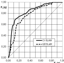
A function is defined by reportingFL(TR)versusFB(TR)
(Fig. 8). In the figure, better model performance would be re-flected as a steeper curve, which indicates larger differences between fractions of catchment and observed landslide area corresponding to a givenTRvalue. The “naive” model, which
predicts that the distribution of slope instability occurs in di-rect proportion to the terrain area mapped for each threshold, is represented in Fig. 8 by the 1 : 1 line. The figure shows that, for a given percentage of basin area with value ofTR
less than the threshold, many more observed landslides fall in the area mapped by CI-SLAM. For instance, 60 % of the observed landslides fall in the 10 % less stable fraction of the basin defined by using CI-SLAM, whereas only 26 % of the landslides fall in the corresponding fraction of the basin de-fined by using QDSLaM. This shows that CI-SLAM provides a better representation of the susceptibility to shallow lands-liding with respect to QDSLaM. At the same time, this quan-tifies the impact that the combination of various hydrological processes (transport in the unsaturated zone, connectivity and soil depth) that are not taken into account by QDSLaM has on shallow landslide triggering.
5 Summary and conclusions
The shallow landslide model developed in this study, CI-SLAM, takes into account both the vertical infiltration in un-saturated soil and the lateral flow in the un-saturated zone in modelling of the local pore-water pressure, and introduces in its framework the concept of hydrological connectivity.
CI-SLAM’s hydrological module is based on the idea that lateral flow occurs when a perched water table develops over the whole upslope area, and identifies a connectivity time for
Fig. 8.Comparison of CI-SLAM and QDSLaM: relationship be-tween cumulative frequenciesFL(TR) andFB(TR)for the study area.
such a condition to be achieved. This connectivity time rep-resents therefore the time lag (from the onset of rainfall) re-quired for a point in the basin to become hydrologically con-nected with its own upslope contributing area. For time less than the connectivity time, vertical infiltration is simulated by using the concept of drainable porosity under the assump-tion of quasi-steady state hydraulic equilibrium. For times greater than the connectivity time, a dynamic topographic in-dex allows us to describe the transient lateral flow dynamics. Moreover, unlike the traditional, lateral flow-dominated, to-pographic index-based models, CI-SLAM is able to account for partial soil saturation, which, in turn, affects the soil shear strength used for modelling slope stability. A spatially vari-able soil depth is the main control of hydrological connectiv-ity in the model.
Model performance was evaluated over three catchments located in the central Italian Alps, where reliable intensity– duration–frequency relationships of extreme rainfall events, detailed inventories of shallow landslides, and estimates of soil depths are available. We found that in the case studies CI-SLAM provides a reasonably correct estimation for fail-ure initiation probability. CI-SLAM has also been compared to the simpler QDSLaM conceptual model, showing better performances in predicting shallow landslide activities, as quantified by the statistical analysis of the results.
Appendix A
Computation of the connectivity timetup
wt as a time of subsurface hydrological connectivity
of the water table timetwt encountered along this flow path.
This highest value is assigned to each new cell encountered downslope until a higher value is encountered. This can be done because of the use of the D8 flow algorithm which as-sumes that each cell has a unique downslope flow direction. Therefore, when a flow path P2 converges in a pre-processed path P1, P2 is terminated if it contains a water table time lower than the encountered water table time in P1. On the other hand, P2 continues downslope to modify P1 with the highest upslope water table time.
Thus, each grid cell in the basin has both atwtvalue, which
indicates the local time for the development of a perched wa-ter table, and a connectivity timetwtup, which defines when a cell is hydrologically connected with its own upslope con-tributing area.
Acknowledgements. This research was funded by the HydroAlp Project and by the Era.Net Circle Project ARNICA. The au-thors thank Jeff Mcdonnell for his comments on an earlier draft. All the codes presented in the article were implemented in R and are freely available by contacting the first author ([email protected]).
Edited by: N. Romano
References
Aberegg, I., Egli, M., Sartori, G. and Purves, R.: Modelling spa-tial distribution of soil types and characteristics in a high Alpine valley (Val di Sole, Trentino, Italy), Studi Trent. Sci. Nat., 85, 39–50, 2009.
Barling, R. D., Moore, I. D., and Grayson, R. B.: A quasi-dynamic wetness index for characterizing the spatial distribution of zones of surface saturation and soil water content, Water Resour. Res., 30, 1029–1044, 1994.
Baum, R. L., Savage, W. Z., and Godt, J. W.: TRIGRS – A FOR-TRAN program for transient rainfall infiltration and grid based regional slope stability analysis, version 2.0, US Geol. Surv. Open File Rep. 2008, 1159, p. 74, 2008.
Beven, K. J. and Kirkby, M. J.: A physically based variable con-tributing area model of basin hydrology, Hydrol. Sci. Bull., 24, 43–69, 1979.
Bierkens, M.: Modeling water table fluctuations by means of a stochastic differential equation, Water Resour. Res., 34, 2485– 2499, 1998.
Borga, M., Dalla Fontana, G., Da Ros, D., and Marchi, L.: Shallow landslide hazard assessment using a physically based model and digital elevation data, J. Environ. Geol., 35, 81–88, 1998. Borga, M., Dalla Fontana, G., Gregoretti, C., and Marchi, L.:
As-sessment of shallow landsliding by using a physically based model of hillslope stability, Hydrol. Process., 16, 2833–2851, 2002a.
Borga, M., Dalla Fontana, G., and Cazorzi, F.: Analysis of topo-graphic and climatologic control on rainfall-triggered shallow landsliding using a quasi-dynamic wetness index, J. Hydrol., 268, 56–71, 2002b.
Borga, M., Tonelli, F., and Selleroni, J.: A physically-based model of the effects of forest roads on slope stability, Water Resour. Res., 40, W12202, doi:10.1029/2004WR003238, 2004. Borga, M., Dalla Fontana, G., and Vezzani, C.: Regional rainfall
depth-duration-frequency equations for an alpine region, Nat. Hazards, 36, 221–235, 2005.
Burlando, P. and Rosso, R.: Scaling and multiscaling models of depth–duration–frequency curves from storm precipitation, J. Hydrol., 187, 45–64, 1996.
Buttle, J. M., Dillon, P. J., and Eerkes, G. R.: Hydrologic coupling of slopes, riparian zones and streams: an example from the Cana-dian Shield, J. Hydrol., 287, 161–177, 2004.
Casadei, M., Dietrich, W. E., and Miller, N. L.: Testing a model for predicting the timing and location of shallow landslide initiation in soil-mantled landscapes, Earth Surf. Proc. Land., 28, 925–950, 2003.
Catani, F., Segoni, S., and Falorni, G.: An empirical geomorphology-based approach to the spatial prediction of soil thickness at catchment scale, Water Resour. Res., 46, W05508, doi:10.1029/2008WR007450, 2010.
Cordano, E. and Rigon, R.: A perturbative view on the subsurface water pressure response at hillslope scale, Water Resour. Res., 44, W05407–W05407, doi:10.1029/2006WR005740, 2008. D’Odorico, P., Fagherazzi G. and Rigon, R.: Potential for
landslid-ing: Dependence on hyetograph characteristics, J. Geophys. Res., 110, F01007, doi:10.1029/2004JF000127, 2005.
Dietrich, W. E., Reiss, R., Hsu, M.-L., and Montgomery, D. R.: A process-based model for colluvial soil depth and shallow land-sliding using digital elevation data, Hydrol. Processes, 9, 383– 400, doi:10.1002/hyp.3360090311, 1995.
Dietrich, W. E., Bellugi, D., and Real de Asua R.: Validation of the shallow landslide model SHALSTAB for forest management, in: Land Use and Watersheds: Human influence on hydrology and geomorphology in urban and forest areas, edited by: Wigmosta, M. S. and Burges, S. J., Am. Geophys. Union Water Sci. Appl., 2, 95–227, 2001.
Freer, J., McDonnell, J. J., Beven, K. J., Peters, N. E., Burns, D. A., Hooper, R. P., Aulenbach, B., and Kendall, C.: The role of bedrock topography on subsurface storm flow, Water Resour. Res., 38, 1269, doi:10.1029/2001WR000872, 2002.
Gessler, P. E., Moore, I. D., McKenzie, N. J., and Ryan, P. J.: Soil landscape modeling and spatial prediction of soil attributes, Int. J. Geogr. Inf. Syst., 9, 421–432, doi:10.1080/02693799508902047, 1995.
Godt, J. W., Baum, R. L., and Lu, N.: Landsliding in par-tially saturated materials, Geophys. Res. Lett., 36, L02403, doi:10.1029/2008GL035996, 2009.
Graham, C. B., Woods, R. A., and McDonnell, J. J.: Hillslope threshold response to rainfall: (1) A field based forensic ap-proach, J. Hydrol., 393, 65–76, 2010.
Grayson, R. B., Western, A. W., Chiew, F. H. S., and Bl¨oschl, G.: Preferred states in spatial soil moisture patterns: local and nonlo-cal controls, Water Resour. Res., 33, 2897–2908, 1997. Heimsath, A. M., Dietrich, W. E., Nishiizumi, K., and Finkel, R. C.:
The soil production function and landscape equilibrium, Nature, 388, 358–361, doi:10.1038/41056, 1997.
doi:10.1016/S0169-555X(98)00095-6, 1999.
Hewlett, J. D. and Hibbert, A. R.: Factors affecting the response of small watersheds to precipitation in humid areas, in: Forest Hydrology, edited by: Sopper, E. E. and Lull, H. W., Pergamon, 275–290, 1967.
Hilberts, A., Troch, P., and Paniconi, C.: Storage-dependent drain-able porosity for complex hillslopes. Water Resour. Res., 41, W06001, doi:10.1029/2004WR003725, 2005.
Hopp, L. and McDonnell, J. J.: Connectivity at the hillslope scale: Identifying interactions between storm size, bedrock permeabil-ity, slope angle and soil depth, J. Hydrol., 376, 378–391, 2009. Keijsers, J. G. S., Schoorl, J. M., Chang, K.-T., Chiang, S.-H.,
Claessens, L., and Veldkamp, A.: Calibration and resolution ef-fects on model performance for predicting shallow landslide lo-cations in Taiwan, Geomorphology, 133, 168–177, 2011. Kirkby, M.: Hydrograph modelling strategies, in: Processes in
Phys-ical and Human Geography, edited by: Peel, R., Chisholm, M., and Haggett, P., Heinemann, London, 69–90, 1975.
Koutsoyiannis, D., Kozonis, D., and Manetas, A.: A mathematical framework for studying rainfall intensity–duration–frequency re-lationships, J. Hydrol., 206, 118–135, 1998.
Lanni, C., McDonnell, J. J., and Rigon, R.: On the relative role of upslope and downslope topography for describing water flowpath and storage dynamics: a theoretical analysis, Hydrol. Process., 25, 3909–3923, doi:10.1002/hyp.8263, 2011.
Lanni, C., McDonnell, J., Hopp, L., and Rigon, R.: Simulated effect of soil depth and bedrock topography on near-surface hydrologic response and slope stability, Earth Surf. Proc. Land, online first: doi:10.1002/esp.3267, 2012.
Lu, N. and Godt, J. W.: Infinite-slope stability under steady un-saturated seepage conditions, Water Resour. Res., 44, W11404, doi:10.1029/2008WR006976, 2008.
Lu, N. and Likos, W. J.: Suction stress characteristic curve for unsat-urated soil, J. Geotech. Geoenviron. Eng., 123, 131–142, 2006. McNamara, J. P., Chandler, D., Seyfried, M., and Achet. S.: Soil
moisture states, lateral flow, and streamflow generation in a semi-arid, snowmelt-driven catchment, Hydrol. Process., 19, 4023– 4038, 2005.
Montgomery, D. R. and Dietrich, W. E.: A physically based model for the topographic control on shallow landsliding, Water Resour. Res., 30, 1153–1171, doi:10.1029/93WR02979, 1994.
Nash, J. E. and Sutcliffe, J. V.: River flow forecasting through conceptual models, J. Hydrol., 10, 282–290, doi:10.1016/0022-1694(70)90255-6, 1970.
Nicotina, L., Tarboton, D. G., Tesfa, T. K., and Rinaldo, A.: Hydro-logic controls on equilibrium soil depths, Water Resour. Res., 47, W04517, doi:10.1029/2010WR009538, 2011.
Pack, R. T., Tarboton, D. G., and Goodwin, C. N.: The SINMAP approach to terrain stability mapping, in: Proceedings – interna-tional congress of the Internainterna-tional Association for Engineering Geology and the Environment 8, v. 2, edited by: Moore, D. P. and Hungr. O., A. A. Balkema, Rotterdam, The Netherlands, 1157– 1165, 1998.
Pelletier, J. D. and Rasmussen, C.: Geomorphically based predictive mapping of soil thickness in upland watersheds, Water Resour. Res., 45, W09417, doi:10.1029/2008WR007319, 2009. Rahardjo, H., Lee, T. T., Leong, E. C., and Rezaur, R. B.: Response
of a residual soil slope to rainfall, Can. Geotech. J., 42, 340–351, doi:10.1139/t04-101, 2005.
Roering, J. E., Kirchner, J. W., and Dietrich, W. E.: Evidence for nonlinear, diffusive sediment transport on hillslopes and implica-tions for landscape morphology, Water Resor. Res., 35, 853–870, 1999.
Rosso, R., Rulli, M. C., and Vannucchi, G.: A physically based model for the hydrologic control on shallow landsliding, Water Resour. Res., 42, W06410, doi:10.1029/2005WR004369, 2006. Saco, P. M., Willgoose, G. R., and Hancock, G. R.: Spatial
organiza-tion of soil depths using a landform evoluorganiza-tion model, J. Geophys. Res., 111, F02016, doi:10.1029/2005JF000351, 2006.
Saulnier, G. M., Beven, K., and Obled, C.: Including spatially vari-able effective soil depths in TOPMODEL, J. Hydrol., 202, 158– 172, doi:10.1016/S0022-1694(97)00059-0, 1997.
Spence, C.: A Paradigm Shift in Hydrology: Storage Thresholds Across Scales Influence Catchment Runoff Generation, Geogr. Compass, 4, 819–833, doi:10.1111/j.1749-8198.2010.00341.x, 2010.
Spence, C. and Woo, M. K.: Hydrology of subarctic Cana-dian shield: soil-filled valleys, J. Hydrol., 279, 151–166, doi:10.1016/S0022-1694(03)00175-6, 2003.
Stieglitz, M., Shaman, J., McNamara, J., Engel, V., Shan-ley, J., and Kling, G.W.: An approach to understanding hy-drologic connectivity on the hillslope and the implications for nutrient transport, Global Biogeochem. Cy., 17, 1105, doi:10.1029/2003GB002041, 2003.
Summerfield, M. A.: Global Geomorphology, Longman, New York, 537 pp. 1997.
Tarolli, P. and Tarboton, D. G.: A new method for determination of most likely landslide initiation points and the evaluation of digi-tal terrain model scale in terrain stability mapping, Hydrol. Earth Syst. Sci., 10, 663–677, doi:10.5194/hess-10-663-2006, 2006. Tarolli, P., Borga, M., and Dalla Fontana, G.:
Analyz-ing the influence of upslope bedrock outcrops on shallow landsliding, Geomorphology, 93, 186–200, doi:10.1016/j.geomorph.2007.02.017, 2008.
Tarolli, P., Borga, M., Chang, K.-T., and Chiang, S. H.: Modeling shallow landsliding susceptibility by incorporating heavy rainfall statistical properties, Geomorphology, 133, 199–211. 2011. Tesfa, T. K., Tarboton, D. G., Chandler, D. G., and McNamara, J. P.:
Modeling soil depth from topographic and land cover attributes, Water Resour. Res., 45, W10438, doi:10.1029/2008WR007474, 2009.
Troch, P.: Conceptual basin-scale runoff process models for humid catchments: Analysis, synthesis and applications, Ph.D. thesis, Ghent Univ., Ghent, Netherlands, 1992.
Tromp-van Meerveld, H. J. and McDonnell, J. J.: Threshold rela-tions in subsurface stormflow: 2. The fill and spill hypothesis, Water Resour. Res., 42, W02411, doi:10.1029/2004WR003800, 2006.
van Genuchten, M. Th.: A closed-form equation for predicting the hydraulic conductivity of unsaturated soils, Soil Sci. Soc. Am. J., 44, 892–898, 1980.
Weiler, M., McDonnell, J. J., Tromp-van Meerveld, H. J., and Uchida, T.: Subsurface stormflow, Encyclopedia of Hydrological Sciences, Wiley and Sons, 2005.
Weyman, D. R.: Measurements of the downslope flow of water in a soil, J. Hydrol., 20, 267–288, 1973.