www.ocean-sci.net/8/419/2012/ doi:10.5194/os-8-419-2012
© Author(s) 2012. CC Attribution 3.0 License.
Ocean Science
Influence of Ross Sea Bottom Water changes on the warming and
freshening of the Antarctic Bottom Water in the
Australian-Antarctic Basin
K. Shimada1, S. Aoki1, K. I. Ohshima1, and S. R. Rintoul2,3,4,5
1Institute of Low Temperature Science, Hokkaido University, Sapporo, Japan 2CSIRO Marine and Atmospheric Research, Hobart, Tasmania, Australia
3Centre for Australian Weather and Climate Research, Hobart, Tasmania, Australia
4Antarctic Climate and Ecosystems Cooperative Research Centre, University of Tasmania, Hobart, Tasmania, Australia 5CSIRO Wealth from Oceans National Research Flagship, Hobart, Tasmania, Australia
Correspondence to:K. Shimada (k [email protected])
Received: 14 October 2011 – Published in Ocean Sci. Discuss.: 2 November 2011 Revised: 11 May 2012 – Accepted: 22 May 2012 – Published: 9 July 2012
Abstract. Changes to the properties of Antarctic Bottom Water in the Australian-Antarctic Basin (AA-AABW) be-tween the 1990s and 2000s are documented using data from the WOCE Hydrographic Program (WHP) and repeated hy-drographic surveys. Strong cooling and freshening are ob-served on isopycnal layers denser than γn= 28.30 kg m−3. Changes in the average salinity and potential temperature be-low this isopycnal correspond to a basin-wide warming of 1300±200 GW and freshening of 24±3 Gt year−1. Recent changes to dense shelf water in the source regions in the Ross Sea and George V Land can explain the freshening of AA-AABW but not its extensive warming. An alternative mech-anism for this warming is a decrease in the supply of AABW from the Ross Sea (RSBW). Hydrographic profiles between the western Ross Sea and George V Land (171–158◦E) were analyzed with a simple advective-diffusive model to assess the causes of the observed changes. The model suggests that the warming of RSBW observed between the 1970s and 2000s can be explained by a 21±23 % reduction in RSBW
transport and the enhancement of the vertical diffusion of heat resulting from a 30±7 % weakening of the abyssal
stratification. The documented freshening of Ross Sea dense shelf water leads to a reduction in both salinity and density stratification. Therefore the direct freshening of RSBW at its source also produces an indirect warming of the RSBW. A simple box model suggests that the changes in RSBW prop-erties and volume transport (a decrease of 6.7 % is assumed
between the year 1995 and 2005) can explain 51±6 % of the
warming and 84±10 % of the freshening observed in
AA-AABW.
1 Introduction
I8S I9S SR3
AAD
PET
3000 4000
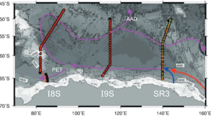
Fig. 1.Locations of the WOCE WHP (black circles) and their repeat (red and green circles) meridional hydrographic sections crossing the Australian-Antarctic Basin with schematic view of spreading path of the AABW. Red circles on SR3 show locations of repeat occupations in the year 2001 (50–61◦S), 2002 (61–66◦S), 2003 (61–66◦S) and green circles show those in 2008, respectively. All the red circles on both I9S and I8S show repeat occupations in the 2000s. Red and blue arrows indicate the RSBW from the Ross Sea and ALBW from the AGVL region respectively and the AA-AABW is indicated by purple arrows.
of brine during sea ice formation in coastal polynyas, over-flow down the continental slope and entrain relatively warm Circumpolar Deep Water (CDW) (e.g. Gordon et al., 2004, 2009; Orsi and Wiederwohl, 2009; Williams et al., 2010).
The nature and causes of changes to AA-AABW have been clarified in several recent studies. Whitworth (2002) concluded that two distinct modes of AA-AABW had been produced in the basin, with the cold, fresh mode more preva-lent in later observations. Jacobs (2004, 2006) concluded that salinity had declined in the region between 140 and 150◦E
south of 65◦S. Aoki et al. (2005) reported a freshening trend at 140◦E from the early 1970s. Using hydrographic sections, Rintoul (2007) showed a freshening of AA-AABW across the entire basin. The distribution of CFC-12 indicated that changes are limited to a ventilated layer that had been in contact with the atmosphere within 55 years (Johnson et al., 2008), consistent with the time-scale of changes reported by Aoki et al. (2005) and Rintoul (2007). Changes in the abyssal layer of the world ocean have been traced back to AABW, with the largest changes seen close to the Antarctic continent (Purkey and Johnson, 2010, 2012). In particular, changes in AA-AABW have been identified as the source of changes in the deep North Pacific (e.g. Kawano et al., 2009; Masuda et al., 2010). Identifying the process driving these changes is therefore an important step in understanding changes in the overturning circulation.
Changes in AA-AABW could reflect changes in the prop-erties, volume transport, and mixing ratios of the dense shelf waters. For example, the wide-spread freshening observed in recent decades could reflect an increased supply of meltwa-ter from ice shelves and glacier tongues. The rapid melt of floating ice in the Amundsen-Bellingshausen Seas has been
identified as the likely source of the strong freshening trend observed in the shelf waters of the Ross Sea (Jacobs et al., 2002; Zwally et al., 2005; Jacobs and Giulivi, 2010). The changes in temperature of AA-AABW have greater spatial variety and are more difficult to explain. AA-AABW warmed over much of the basin between the years 1936–1993 and 1994–1996 (Whitworth, 2002), but cooled in the region be-tween 140 and 150◦E from the 1950 to 2001 (Jacobs, 2004, 2006) and at 140◦E between the 1970s and 2002 (Aoki et al., 2005), although the magnitude of the trend may be aliased by higher-frequency signals. These overall changes in tempera-ture with space and time suggest that the relative contribution of different source waters may have also played a role in the observed changes of AA-AABW.
Several studies suggest that changes in RSBW and its source waters are likely to have contributed to the changes observed in the Australian-Antarctic Basin. Jacobs (2006) and Rintoul (2007) showed a consistent freshening of RSBW between the Ross Sea outflow and 150◦E. Freshening of shelf waters in the Ross Sea have been attributed in part to the inflow of glacial meltwater from the east (Jacobs et al., 2002; Jacobs and Giulivi, 2010). Changes in sea ice forma-tion are also likely to have played a role. Tamura et al. (2008) inferred a 30 % reduction in the volume of sea ice formed in the Ross Ice Shelf Polynya region from the end of the 1990s to the 2000s. Rivaro et al. (2010) estimated that the export of dense water from the western Ross Sea in 2001 and 2003 are 45 % and 30 % lower than that in 1997, respectively, although these estimates may be subject to aliasing due to higher-frequency variability. Therefore, change in both the properties and volume transport of RSBW may have con-tributed to observed changes in AA-AABW downstream.
In this study, we describe changes in AA-AABW proper-ties based on CTD profiles of the WOCE Hydrographic Pro-gram (WHP) surveys in the 1990s and later repeat surveys in the 2000s. Historical observations are used to track changes in RSBW from the 1970s to the 2000s. A simple advective-diffusive model of downstream evolution of RSBW is then developed to determine the contribution of changes in trans-port and mixing to its observed changes. Finally, the influ-ences of changes in both RSBW properties and volume trans-port on AA-AABW are assessed.
2 Changes to AABW in the Australian-Antarctic Basin 2.1 Water mass properties
−0.8 −0.6 −0.4 −0.2 0.0
65 60 55
34.64 34.66 34.68 34.70
28.28 28.30 28.32 28.34 28.36 −0.6
−0.4 −0.2 0.0
65 60 55
34.66 34.68
28.28 28.30 28.32 28.34 28.36
115 120 125 130 −0.4
−0.2 0.0
66 65 64 63 58 56 54 52 50 48
34.66 34.67 34.68 34.69
28.28 28.30 28.32 28.34 28.36
115 120 125 130
(
a)
I
8S
(
b)
I
9S
(
c) SR3
Fig. 2.Meridional variations of the water properties averaged over the 100 m-thick layer at the bottom for(a)I8S,(b)I9S and(c)SR3. Blue circles and lines are from the WHP occupations in the 1990s. Red circles and lines in(c)are from repeat occupations in the year 2001 (50–61◦S), 2002 (61–66◦S), 2003 (61–66◦S) and green circles and lines in(c)are from those in 2008. All the red circles and lines in both (a)and(b)are from repeat occupations in the 2000s.
Table 1.Summary of the WOCE WHP and repeat occupations. The WOCE WHP section designation, years and months and latitudinal range of the WHP and repeat occupations, cruise code names, vessels used for repeat occupations and time intervals.
WOCE WHP sections
WHP occupa-tion months and year
WHP occupa-tion latitudinal range
Repeat occupa-tion months and year
Repeat occupa-tion latitudinal range
Repeat occupation cruise – R/V
Time interval (year)
SR3 Jan–Feb 1995 50–66◦S Oct–Nov 2001/
Feb 2002, 2003
50–61◦S/ 61–66◦S
AU0103
– RSV Aurora Australis/ JARE43, 44 Tangaroa
6/ 7, 8
Mar–Apr 2008 50–66◦S AU0806
– RSVAurora Australis
13
I9S Jan 1995 50–66◦S Jan 2005 50–66◦S AU0403
– RSVAurora Australis
10
I8S Dec 1994/
Jan 1995
47–64◦S/ 64–66◦S
Feb–Mar 2007 47–66◦S US Repeat Hydrography Program – R/V Roger Revelle
12
1999). AA-AABW exits the basin through the Princess Elisa-beth Trough (PET) and the Australian-Antarctic Discordance (e.g. Rintoul, 2007; Johnson et al., 2008). The WHP sec-tions (I8S, I9S, and SR3 at 82–93◦E, 115◦E and 140◦E, re-spectively) cross the boundary currents transporting the AA-AABW away from the source regions, and each of these sec-tions was conducted in the 1990s and repeated in the 2000s (Table 1). In this section, we describe changes in bottom wa-ter properties based on these data.
The SR3 section crosses the AA-AABW path at 140◦E, just downstream of the inflow of ALBW at ∼142◦E.
Be-cause this line is close to this dense shelf water source, the near-bottom temperature and salinity on the continental slope and rise vary with season and location (e.g. Fukamachi et al.,
a)
I
8S
b)
I
8S
c)
I
9S
d)
I
9S
e) SR3
θ
(
deg
.)
θ
(
deg
.)
Salinity Salinity
Salinity
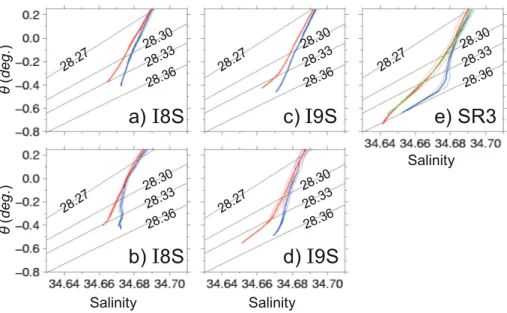
Fig. 3.Variations ofθ-S curves for(a)I8S (46–60◦S, the Australian-Antarctic Basin),(b)I8S (60–67◦S, the PET),(c)I9S (50–61◦S), (d)I9S (61–66◦S) and(e)SR3. Data are averaged on the isopycnal surfaces. Means are shown by thick lines and one standard deviation envelopes are shown by thin lines (following Johnson et al., 2008). Blue lines are from the WHP occupations in the 1990s. Red lines in (e)are from repeat occupations in the year 2001, 2002, 2003 and green lines in(e)are from in the year 2008. All the red lines in other panels are from repeat occupations in the 2000s. Labeled black lines are contour of neutral density (kg m−3).
Decadal changes in the AA-AABW are examined by com-paring the meridional variation of potential temperature (◦C), salinity, neutral density (γnkg m−3) and apparent oxygen utilization (AOU µmol kg−1) averaged over a 100 m-thick layer at the bottom (Fig. 2). At SR3, the potential temper-ature is lower in 2001 and 2008 (by up to 0.1◦C) than in the WHP in the 1990s south of 62◦S. However, the lowest po-tential temperature (−0.72◦C) was in 2001 and the potential
temperature in 2008 (−0.64◦C) was comparable to that of
the WHP in the 1990s. Such a non-monotonic change sug-gests interannual variability in potential temperature. Cool-ing (−0.06◦C) was also observed near 63◦S at I9S.
How-ever, warming (up to 0.1◦C) is found further downstream
along the entire I8S section and north of 61◦S along I9S.
The reversal of sign in the potential temperature changes is also observed in AOU: cooling is associated with a decrease in AOU along I9S south of 62◦S, and warming is associated with an increase in AOU at along I8S and north of 62◦S on I9S (Fig. 2b). While the changes in salinity do not reverse in sign, the freshening trend is intensified closer to the source region near SR3 and at higher latitudes (up to 0.02). In ad-dition, the bottom layer along SR3 is fresher in 2001 than in 2008 (the minimum salinity south of 62◦S is lower by 0.01). Hence, salinity is also observed to vary interannually. There is no clear change of density near the source of dense water south of 62◦S on SR3 and near 63◦S on I9S, because cooling and freshening compensate each other. Further downstream at I8S, and north of 61◦S on I9S, freshening and warming
produces a decrease in density (∼0.02 kg m−3).
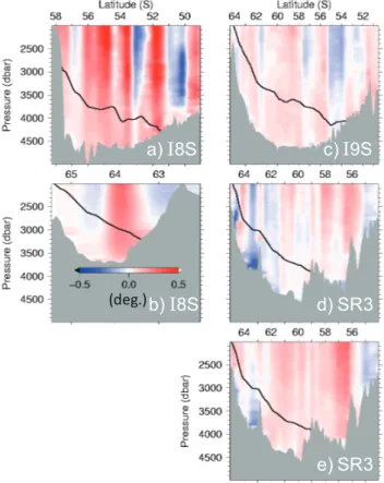
Cooling and freshening on isopycnals reflects warming and/or freshening of water masses where the stratification is such that warmer, more saline waters overly cooler, fresher waters (i.e. density ratio>1, Bindoff and McDougall, 1994). Here cooling and freshening is evident on isopycnal surfaces for water denser thanγn=28.30 kg m−3(Fig. 3), indicating basin-wide warming and/or freshening of the AA-AABW. Property differences on isobaric surfaces indicate spatially different patterns between potential temperature and salinity (Figs. 4 and 5). At SR3, the strongest cooling is observed at the sea floor between 63◦S and 64◦S (Fig. 4d, e). At I9S, warming dominated an∼800 m thick layer belowγn=
28.30 kg m−3, although weak cooling was detected over the slope south of 62◦S (Fig. 4c). Freshening dominates
every-where below γn=28.30 kg m−3 with the strongest fresh-ening at the sea floor (Fig. 5c). At I8S, warming (Fig. 4a, b) and moderate freshening (Fig. 5a, b) are observed below
γn=28.30 kg m−3.
In summary, following the flow path of the AA-AABW, warming increases downstream and the freshening increases upstream. We estimate the heat and freshwater fluxes needed to explain the observed patterns of change by interpolating the changes observed at each section to the entire basin, us-ing a Gaussian weightus-ing function with an e-foldus-ing scale of 300 km and an influence radius of 1000 km. We find the overall warming of AA-AABW requires an input of 1300±
200 GW of heat (or 0.37±0.05 W m−2) and 24±3 Gt year−1
Table 2.Basin and section averaged trends in property of the AA-AABW.(a)Total volume of layers belowγn=28.30 kg m−3isopycnal, area of the Australian-Antarctic basin, mean potential temperature trend, required heat flux, mean salinity trend, required freshwater input in the Australian-Antarctic Basin.(b) Section averaged thickness of layers belowγn=28.30 kg m−3 isopycnals, potential temperature trends, required heat fluxes, salinity trends, required freshwater inputs for respective sections. Error ranges for SR3 were derived from 95 % confidence limit of linear regression coefficient.
(a)
Australian-Antarctic Basin
Volume (km3) 2.54×10⁶ Area (km2) 3.55×10⁶ 1θ(◦C decade−1) 4.09±0.53×10⁻²
Heat input 1322±172 (GW)/0.37±0.05 (W m−2) 1S(decade−1) −2.67±0.42×10⁻³
Fresh water input (Gt year−1)
24.0±3.2
(b)
I8S (40–60◦S)
I8S (60–67◦S)
I9S SR3
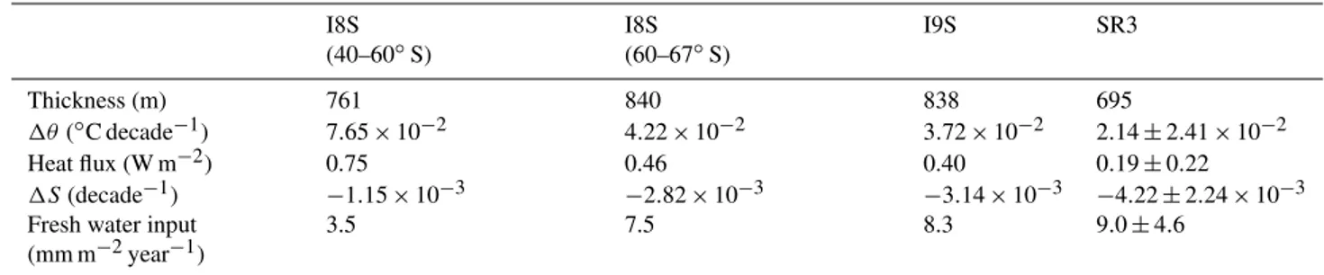
Thickness (m) 761 840 838 695
1θ(◦C decade−1) 7.65×10⁻² 4.22×10⁻² 3.72×10⁻² 2.14±2.41×10⁻²
Heat flux (W m−2) 0.75 0.46 0.40 0.19±0.22
1S(decade−1) −1.15×10⁻³ −2.82×10⁻³ −3.14×10⁻³ −4.22±2.24×10⁻³ Fresh water input
(mm m−2year−1)
3.5 7.5 8.3 9.0±4.6
2.2 Potential mechanisms of the observed changes
Perhaps the most obvious candidate responsible for the ob-served freshening is a decrease in salinity of the dense shelf waters, as observed in the Ross Sea (−0.03 decade−1since
the 1960s, Jacobs and Giulivi, 2010). Freshening by up to−0.01 decade−1 is also observed in the George V Land
(G. D. Williams, personal communication, 2012). However, this mechanism cannot explain the warming of AA-AABW, since the warming of the Ross Sea dense shelf water is small (2×10⁻³◦C decade−1) and has been solely attributed to the
change in freezing point temperature induced by the rapid freshening (Jacobs and Giulivi, 2010).
Other possible causes of warming include geothermal heat flux, horizontal/vertical diffusion, and reduced supply of cold dense shelf waters. Assessing these candidates in or-der, we find the average geothermal heat flux for depths of 3500 to 4500 m is roughly 0.05–0.1 W m−2 (Stein and Stein, 1992). Even a 50 % increase would only account for less than 15 % of the warming of AA-AABW and there is no reason to expect the geothermal heat flux to increase rapidly on decadal time-scales. Horizontal diffusion is ex-pected to carry a heat flux of about 0.01 W m−2, using a basin-averaged horizontal potential temperature gradient on
γn=28.30 kg m−3(8.9×10⁻⁷◦C m−1) and a horizontal
dif-fusivity of 2 m2s−1(e.g. Ledwell, 1998). This is insignificant
relative to the observed warming. Polzin and Firing (1997) estimated a vertical diffusivity of 4.4×10⁻⁴m2s−1at 55◦S
on I8S averaged below 1000 m. The basin-averaged verti-cal potential temperature gradient onγn=28.30 kg m−3is 3.8×10⁻⁴◦C m−1, implying a vertical diffusive heat flux of
0.67 W m−2. Changes in the basin-averaged density stratifi-cation, which can affect both horizontal and vertical diffu-sion, were less than 10 % during the observational period. An increase in vertical diffusion of 10 % would explain only 19 % of the warming over the entire AA-AABW layer. (Den-sity stratification is an important parameter in considering mixing (e.g. Gregg, 1989). As discussed in Sect. 3, changes in the region downstream of the Ross Sea are found to be im-portant, although the change averaged over the entire basin is relatively small.) Overall, none of these processes result in a sufficient change in heat flux to explain the observed warm-ing.
a)
I
8S
b)
I
8S
c)
I
9S
d) SR3
e) SR3
(deg.)
Fig. 4.Difference in isobaric potential temperature between the WHP and repeat occupations. Red areas indicate warming and blue areas indicate cooling. (a) I8S (the Australian-Antarctic Basin), (b)I8S (the PET),(c)I9S,(d)SR3 (obtained from subtracting the WHP from combined repeat occupations in the year 2001, 2002, and 2003),(e)SR3 (obtained from subtracting the WHP from repeat occupations in the year 2008). Meanγn=28.30 kg m−3isopycnals are shown by solid lines.
potential heat/freshwater sources and the spatial distribution of changes, we hypothesize that a reduction in the inflow of RSBW was the major contributing factor to the changes ob-served in the AA-AABW. To examine this possibility in more detail, we consider an advective-diffusive balance for the wa-ters between the western Ross Sea and 150◦E.
3 Advection-diffusion process of RSBW, and its impact on AA-AABW
3.1 Changes in RSBW
The RSBW that supplies the Australian-Antarctic Basin pri-marily forms on the continental rise of the western Ross Sea from overflows of modified shelf water (hereafter MSW) that originate from the Drygalski Trough and mix with CDW (Gordon et al., 2004, 2009; Orsi and Wiederwohl, 2009). It then migrates westwards around Cape Adare, inshore of the Balleny Islands and into the Australian-Antarctic Basin,
a)
I
8S
b)
I
8S
c)
I
9S
d) SR3
e) SR3
(PSS-78)
Fig. 5. Difference in isobaric salinity between the WHP and re-peat occupations. Red areas indicate increase in salinity and blue areas indicate freshening.(a)I8S (the Australian-Antarctic Basin), (b)I8S (the PET),(c)I9S,(d)SR3 (obtained from subtracting the WHP from combined repeat occupations in the year 2001, 2002, and 2003),(e)SR3 (obtained from subtracting the WHP from repeat occupations in the year 2008). Meanγn=28.30 kg m−3isopycnals are shown by solid lines.
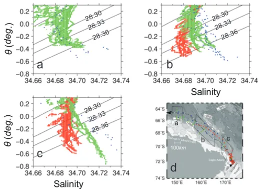
where it is joined by ALBW after 150◦E. To examine the property changes along this approximate flow path, we ex-tracted summer (January to March) hydrographic profiles be-tween the Drygalski Trough of the Western Ross Sea and 150◦E from World Ocean Database 2009 (Boyer et al., 2009). A total of 256 profiles that went to within 50 m of the bottom were available, spanning the period from 1969 to 2004 (Fig. 6d). RSBW freshened consistently from the 1970s and the bottom-intensified salinity maximum was strongly attenuated in the 2000s throughout the study area around 150◦E (Fig. 6a), 160◦E (Fig. 6b), and in the vicinity of the
100km
Drygalski Trough
Cape Adare George V Land Coast
-500
-500
Balleney Islands
a
b
c
d
Salinity
Salinity
θ
(
d
e
g
.)
θ
(
d
e
g
.)
28.30 28.33
28.36
28.30 28.33
28.36
28.30 28.33
28.36
a
b c
Fig. 6.θ-Sdiagrams of region between the Drygalski Trough and 150◦E.(a)around 150◦E,(b)around 160◦E,(c)immediately downstream of the Ross source region,(d): locations of stations. Blue circles are from occupations in the 1970s, green circles are from 1990s and red circles are from 2000s. Labeled black lines in(a), (b), and(c)are contour of neutral density (kg m−3). Dashed arrow in(d) indicates approximate position of flow path of the RSBW and white circles are marked on 100 km interval.
in the 2000s (118.1 µ mol kg−1) compared to that in 1970s (114.1 µ mol kg−1; not shown). The freshening of RSBW can be explained by freshening of its dense water source, but not its warming (2×10⁻³◦C decade−1). However a decrease in
volume transport of RSBW reduces the supply of both cold and oxygen rich water throughout its flow path, consistent with the property changes between the Drygalski Trough and 150◦E.
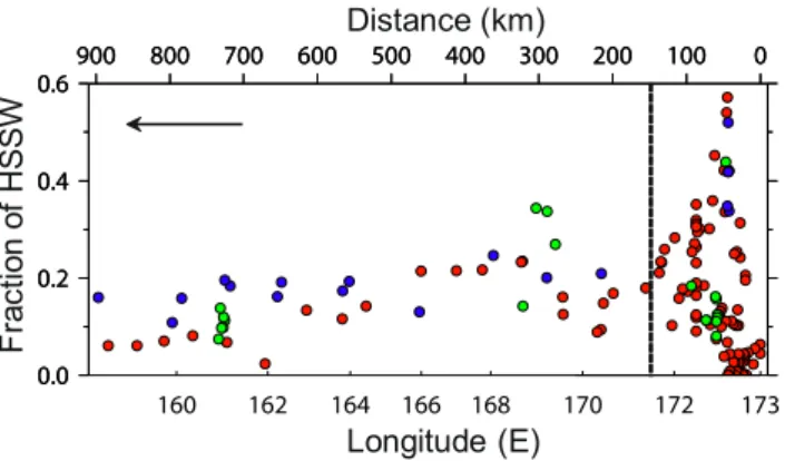
To examine the flow regime and derive the temporal change of RSBW, the mixing process is studied using Op-timum Multiparameter analysis (OMP) to calculate the rela-tive contributions to RSBW of the dense shelf water exported from the Drygalski Trough (hereinafter termed High Salinity Shelf Water, HSSW) and the Lower Circumpolar Deep Wa-ter (LCDW). See Appendix A for details. In both the 1970s and 2000s, most of the profiles in the upstream region within 150 km (east of 171◦E) of the Drygalski Trough showed high HSSW fractions>0.4 (Fig. 7). In the downstream region be-yond 150 km, it is less than 0.2. This rapid decrease suggests that the intensive mixing process including entrainment gov-erns the properties of MSW, i.e. the mid-slope precursor to AABW, within the upstream region, and that the final proper-ties of RSBW become stable at around 150 km downstream. Thus, the upstream region less than 150 km from the Dry-galski Trough is categorized as the region of the intensive modification/formation of MSW into RSBW and the down-stream region beyond 150 km is categorized as the flow path
of RSBW after vigorous mixing. Hereafter, the former region is referred to as the modification path of MSW and the latter to as the flow path of RSBW.
The availability of observational data is important. Along the modification path of the MSW, profiles showing low HSSW fractions are mostly from the 2000s. Although this may reflect decreased HSSW export in the 2000s, the spatial density of the profiles is extremely low in the 1970s com-pared to that of the 2000s. To avoid an error due to this spatial aliasing, we only analyze the flow path of the RSBW where the spatial density of the profiles is equivalent between the 1970s and 2000s. We will further exclude the region beyond 900 km (west of 158◦E) from the Drygalski Trough where there are no observations in the 2000s. Hence, we consider changes in RSBW along its flow path in the region 150– 900 km (171–158◦E) from the Drygalski Trough, between the 1970s and 2000s.
3.2 An advection-diffusion model of RSBW transport
0.0 0.2 0.4 0.6
0 100 200 300 400 500 600 700 800 900
173 172 170 168 166 164 162 160 0.0
0.2 0.4 0.6
0 100 200 300 400 500 600 700 800 900
Longitude (E) Distance (km)
F
ra
ct
io
n
o
f
H
S
S
W
Fig. 7.Distribution of fraction of the HSSW within 100 m from bottom along flow path of the RSBW estimated by OMP analy-sis. Blue circles are from occupations in the 1970s, green circles are from 1990s and red circles are from 2000s. An arrow indicates downstream direction of RSBW and vertical dashed line separates modification path of MSW and flow path of RSBW. See text for definition of paths.
simple model to analyze the long-term changes in advection-diffusion processes of the RSBW in this sector.
The governing diffusion equation of the potential temper-ature of RSBW can be written as follows.
θt+uθx+vθy+wθz=
∂
∂xKhθx+ ∂
∂yKhθy+ ∂ ∂zKzθz,
wherexis the flow path coordinate (downstream positive),y
is the direction orthogonal to the flow path, andzis the ver-tical axis (upward positive).KzandKhare the vertical and
horizontal diffusivities, respectively, with subscripts indicat-ing the first order derivatives.
Starting from this general formula, we will simplify this equation based on the settings and approximations applicable in this case. As shown in Fig. 8, the flow path of the RSBW is bounded by the continental slope and sea floor in the di-rection of y and z, respectively, and the fluxes through these two boundaries are zero. Hence, the horizontal diffusion term of the y-axis and the vertical diffusion term are replaced by the fluxes from the other side divided by the widthLoand thicknessHof RSBW, respectively.
θt+uθx+vθy+wθz=
∂
∂xKhθx+
1
LoKhθy+ 1
HKzθz. (1)
The third and fourth terms on the left hand side can be ne-glected since the velocity orthogonal to the flow path and the vertical velocity are negligible. The first term on the right hand side can be neglected because the horizontal gradient in the x-direction is negligible compared to gradients in the y-and z-directions. Equation (1) can therefore be simplified to:
θt+uθx=
1
LoKhθy+ 1
HKzθz. (2)
Here, we will consider the relative importance of the first and second terms on the right hand side. From Fig. 8, the widthLoand thicknessHof the RSBW can be estimated as 200 km and 200 m, respectively, and the horizontal and verti-cal gradients were estimated asθy≈2.6×10⁻⁶◦C m−1and
θz≈7.0×10⁻⁴◦C m−1, respectively. Setting the vertical
dif-fusivity is a challenge because it has not been determined for this study area. Muench et al. (2009) estimated it in the vicin-ity of the Drygalski Trough but not for the remaining area downstream. However, Kunze et al. (2006) estimated an av-erage vertical diffusivity for the Southern Ocean by using the strain from CTD profiles and the vertical velocity shear from Lowered acoustic Doppler current profiler. From Fig. 16 of Kunze et al. (2006), the near bottom vertical diffusivity can be in the orders of between 10−5–10−4m2s−1. Adopting Os-born’s (1980) model, vertical diffusivityKzcan be written in
the form of
Kz=0.2
ε
N2, (3)
where 0.2 is the mixing efficiency,εis the energy dissipation rate, andNis the Brunt-V¨ais¨al¨a frequency. Here, we simply assume that ε to be constant over decadal or longer time-scale since the energy provided to larger spatial time-scale motion (e.g. tides), which provides energy to turbulence, is constant (note-validity of this assumption will be discussed later).N2
can be calculated from observed vertical profiles using
N2=g(βSz−αθz)∵g= −9.8 m s−2, (4) whereα is the thermal expansion rate and β is the saline contraction rate. With the assumption of constantε, the rate of temporal change in Kz can be estimated by
calculat-ing N2 for each period. Here, by using the vertical diffu-sivity of Kunze et al. (2006), the vertical flux has a value of 3.5×10⁻¹¹–3.5×10⁻¹⁰◦C s−1. By usingKh=2 m2s−1
(e.g. Ledwell, 1998), horizontal flux takes value of 2.6×
10−11◦C s−1. Hence, the vertical diffusion term is likely to be one order of magnitude larger than the horizontal diffu-sion term. Therefore we neglect the horizontal diffudiffu-sion term to obtain the formula as
θt+uθx=
1
HKzθz.
Now we will consider the uniform current (u >0) along the flow path of RSBW. There is no direct observation of u, but Fukamachi et al. (2000) measured current speed of 14.1 to 19.8 cm s−1 at 140◦E, slightly downstream of the cur-rent region of focus. If we assume the above value for the RSBW current speed, the advection time of its signal along the 750 km of its flow path is 42 to 62 days. For the time scale of multi-decadal variability, temperature variations in both time and space in this region are in the order of 0.1◦C, and, hence, our formula becomes
θz
θx
=uH
Kz
Distance (km) Distance (km)
a
b
c
Latitude (S) Latitude (S)
y z
y z
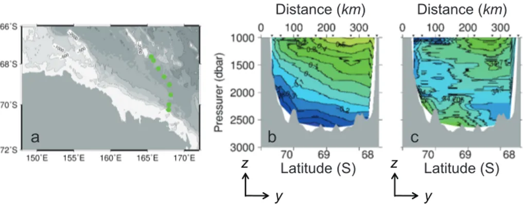
Fig. 8.Thickness and width (cross shore) of the RSBW from occupations in the 1990s.(a)Location of stations,(b)vertical cross section of potential temperature,(c)vertical cross section of salinity.yis cross shore coordinate (offshore positive), andzis vertical axis (upward positive). Thickness and width of cold and saline the RSBW are approximately 200 m and 200 km, respectively.
for each period of interest. The assumed current speeds are likely faster than the RSBW due to the input of ALBW at
∼142◦E. However, even if we assume a half of the
cur-rent speed, the scaling that θt is negligible remains valid.
Given Eq. (5), we can estimate the volume transportuH for a certain period by estimatingθx,θz, andN2based on the
observed hydrographic profiles, and thereafter the decadal change ofuH can also be obtained.
Note that Eq. (5) implies that the ratio of the vertical gradi-ent to the horizontal gradigradi-ent is determined by the ratio of the volume transport to the vertical diffusivity. Horizontal veloc-ityuis relevant to the residence time in the benthic box, and a largeuacts to enhance the contrast between the RSBW layer and overlying water, i.e. producing a larger vertical gradient. ThicknessH determines the total volume of the RSBW, and hence a larger H acts to enhance the vertical gradient be-tween the RSBW and overlying layers. Hence, when the vol-ume transportuH is large, the vertical gradientθzshould be
large (and/or horizontal gradientθxshould be small). IfuH
is small,θzis small (and/orθxis large). Conversely, large
ver-tical diffusivityKztends to reduce the vertical gradient and
thus, acts in the opposite sense touH.
The diffusion equation for salinity is also given in this manner. Then, Eq. (5) is expressed as
uH=Kz
θz
θx =Kz
Sz
Sx
(6)
By substituting Eq. (3) into Eq. (6), we have the following equation.
uH∗= 1
N2 θz θx = 1 N2 Sz Sx (7)
whereuH∗=uH /0.2ε. In the next subsection, we discuss change of volume transport by applying Eq. (7) to each re-spective period.
Distance (km)
Longitude (E)
Sa
lin
it
y
S
z(1
0
- 5m
- 1)
34.68 34.71 34.74 34.77 200 300 400 500 600 700 800 900 34.68 34.71 34.74 34.77 200 300 400 500 600 700 800 900 34.68 34.71 34.74 34.77 200 300 400 500 600 700 800 900 34.68 34.71 34.74 34.77 200 300 400 500 600 700 800 900 34.68 34.71 34.74 34.77 200 300 400 500 600 700 800 900 −30 −25 −20 −15 −10 −5 0 −30 −25 −20 −15 −10 −5 0 −30 −25 −20 −15 −10 −5 0 170 168 166 164 162 160−0.6 −0.5 −0.4 −0.3 −0.2
1960 1970 1980 1990 2000 2010
−0.6 −0.5 −0.4 −0.3 −0.2
1960 1970 1980 1990 2000 2010
34.68 34.69 34.70 34.71 34.72 34.73
34.68 34.69 34.70 34.71 34.72 34.73
S
a
lin
it
y
θ
(
d
e
g
.)
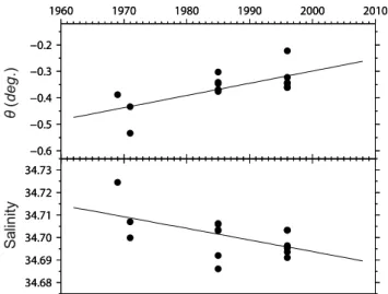
Fig. 10.Potential temperature (upper panel) and salinity (lower panel) averaged over the 100 m-thick layer at the bottom vs. year with regression lines from region around 150◦E. Profiles locate within box(a)in Fig. 6d are used here.
Table 3.Mean vertical salinity gradients, horizontal salinity gra-dients, their ratios,N2anduH∗ for the RSBW in the 1970s and 2000s from region between 150 km and 900 km downstream from the Drygalski Trough.
1970s 2000s
Sz (m−1) −8.94±0.71×10⁻⁵ −3.71±0.24×10⁻⁵ Sx (m−1) −3.86±0.59×10⁻⁸ −2.90±0.62×10⁻⁸
Sz/Sx 2300±400 1300±300
N2(s−2) 1.91±0.17×10⁻⁶ 1.34±0.05×10⁻⁶ uH∗(s2) 12.1±2.3×10⁸ 9.5±2.2×10⁸
3.3 Changes in the advection-diffusion process of RSBW
The data along the flow path of RSBW into the Australian-Antarctic Basin (171–158◦E, i.e. downstream region be-tween 150–900 km from the Drygalski Trough) are used to examine change in the volume transport of RSBW between the 1970s and 2000s. In practice, the relative contribution of the large-scale pattern and small-scale variability along the flow path of the RSBW are different for temperature and salinity near the source region. While the large-scale pat-tern of temperature and its gradient are subject to signifi-cant small-scale perturbations, those of salinity and its gra-dient are dominant over small-scale spatial variations. This tendency becomes more prominent in the 2000s because the salinity contrast between the ambient water is reduced over this period due to the freshening of the RSBW, while the po-tential temperature contrast remained relatively unchanged. Hence, we conduct further analysis based on salinity
aver-aged over the 100-m thick layer at the bottom and vertical gradients (Fig. 9).
We will now focus on the treatment of data and their application to the model. To ensure all the areas are uni-formly weighted, horizontal gradients were estimated by a least squares fit to the data averaged in 50 km interval bins for the two periods. Horizontal gradients of salinity in the 1970s and 2000s are estimated as−3.86±0.59×10⁻⁸m−1
and−2.90±0.62×10⁻⁸m−1, respectively (Table 3). Thus,
the change in horizontal gradient from the 1970s to 2000s is estimated to present a ∼25 % decrease. Vertical
gradi-ents in 1970s and 2000s are estimated by taking the mean of bin averages (i.e. the mean of the larger circles in the lower panels of Fig. 9) as −8.94±0.71×10⁻⁵m−1 and −3.71±0.24×10⁻⁵m−1, respectively. The change in
ver-tical gradient by far exceeds that of the horizontal gradient and is estimated as a∼59 % decrease. Accordingly, the ra-tios of vertical to horizontal gradient in 1970s and 2000s are estimated as 2300±400 and 1300±300, respectively, and
present a decrease of∼45 %. From Eq. (4),N2in 1970s and 2000s are 1.91±0.17×10⁻⁶s−2and 1.34±0.05×10⁻⁶s−2
respectively, and as such is a∼30 % decrease. Substituting
these estimates for Eq. (7),uH∗in the 1970s and 2000s are estimated as 12.1±2.3×10⁸s2and 9.5±2.2×10⁸s2,
respec-tively. Hence, the temporal change inuH∗from the 1970s to the 2000s is estimated as a decrease of 21±23 %, although
it is subjected to a large uncertainty.
These results suggest a reduction in the volume transport of the RSBW is associated with enhanced vertical diffusion, as a result of weakening in the stratification (the decrease in
N2is sufficient to increase the vertical diffusivity by 42 %). A reduction in volume transport is also consistent with the observed warming and increase in AOU of the RSBW. 3.4 Impact of RSBW on AABW in the
Australian-Antarctic Basin
The property changes of the RSBW are evident from the ob-servations (Sect. 3.1) and a decrease in its volume transport is also suggested (Sects. 3.2–3.3). Now we examine the in-fluence of both of these processes on the bottom water prop-erties in the basin as a whole (AA-AABW), using a simple box model under some realistic assumptions.
The change in potential temperature of the AA-AABW, due to the supply of RSBW per unit time, can be represented as
−1
VVtr1θ, (8)
where Vtr is volume transport of the RSBW supplied to
the Australian-Antarctic Basin, 1θ is difference in poten-tial temperature between the RSBW and the AA-AABW, andV is total volume of the AA-AABW. Here,Vtrand1θ
time, i.e.,Vtr=Vtr+δVtrtand1θ=1θ+δθ t. Substitution
of these into Eq. (8) gives,
−1
V(Vtr1θ+Vtrδθ t+1θ δVtrt+δθ δVtrt
2).
(9) The first term in the brackets is the steady state component, which is assumed to be balanced with the steady state heat flux in the basin due to vertical and horizontal diffusion and geothermal heat.V is kept constant in this formulation (see Sect. 4). Here we are interested in the fluctuation compo-nents that deviate from the balance, and thus, we neglect the first term and the fourth infinitesimal term. By integrating the above equation with respect to time, the warming of the AA-AABW due to the RSBW influence (1θRSBW) by temporal
changes in property and volume transport can be considered. The corresponding freshening of the AA-AABW due to the RSBW influence (1SRSBW) is also given by the same
proce-dure. For the integrating timeT, we now have
1θRSBW= −
1
V(Vtrδθ+1θ δVtr) T2
2
1SRSBW= −
1
V(VtrδS+1SδVtr) T2
2 (10)
The first term on the right hand side of Eq. (10) is the com-ponent due to the changes in property of the RSBW and the second term is the component due to the decrease in its vol-ume transport.
The contributions of temperature and salinity changes from the RSBW are then estimated using Eq. (10) for the 10 year period from 1995 to 2005, following the observa-tional period in the Australian-Antarctic Basin. The trend in potential temperature and salinity of the RSBW is eval-uated using the regression lines for the bottom water proper-ties averaged over a 100 m-thick bottom layer around 150◦E (Fig. 10). The potential temperature and salinity of the AA-AABW in the years 1995 and 2005 are calculated as a basin average estimated using all data shown in Table 1 and the trends shown in Table 2a, respectively. These averages are estimated by the same interpolation procedure as that in Sect. 2.1. Then,δθ andδS, the changing rate of difference between the RSBW and the AA-AABW, are estimated as
δθ=1θ2005−1θ1995
T , δS=
1S2005−1S1995
T
The steady state component of the RSBW volume transport
Vtr is required in this formulation. Here we use 7 Sv as a
reference with an average westward velocity of 17.5 cm s−1 over the area of width and thickness of 200 km and 200 m, respectively, at 150◦E (note – the validity of this estimate will be discussed later).
With the aboveVtr and observedδθ andδS, the change
in property of the RSBW can explain 44±5 % and 63±8 %
of observed warming and freshening of the AA-AABW. The change rate of volume transportδVtris the largest unknown
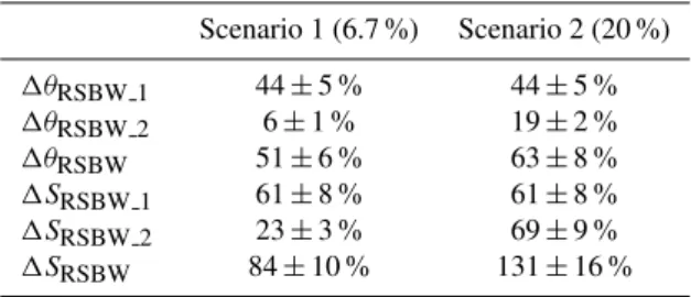
Table 4.Possible warming and freshening of the AA-AABW in-duced by change in property, decrease in volume transport of the RSBW, and their summations under the two scenarios of volume transport decrease of 6.7 %/10 years and 20 %/10 years. Results are shown in the form of ratio to the overall warming and freshening of the AA-AABW estimated in Sect. 2. Subscripts “1” denote contri-bution by change in property (first term in right hand side of Eq. 10) and subscript “2” denote contribution by decrease in volume trans-port of the RSBW (second term in right hand side of Eq. 10).
Scenario 1 (6.7 %) Scenario 2 (20 %)
1θRSBW 1 44±5 % 44±5 %
1θRSBW 2 6±1 % 19±2 %
1θRSBW 51±6 % 63±8 %
1SRSBW 1 61±8 % 61±8 %
1SRSBW 2 23±3 % 69±9 %
1SRSBW 84±10 % 131±16 %
in Eq. (10). Hence, we consider possible two scenarios. In scenario 1, we assume that there was a 6.7 % decrease in the volume transport of the RSBW from 1995 to 2005. This value is based on the suggested decrease in volume transport of the RSBW (≈20 %/30 years) derived in Sect. 3.2. For the
scenario 2, we assume a 20 % decrease of RSBW volume transport, which reflects the rapid decrease in sea ice produc-tion described by Tamura et al. (2008) over this period.
Hereafter we evaluate 1θRSBW and 1SRSBW using
Eq. (10) according to these two scenarios for the decrease in volume transport (Table 4). For scenario 1,1θRSBW can
explain 51±6 % of the overall warming of the AA-AABW.
The contribution of the change in property (first term) by far exceeds that of the change in volume transport (second term).1SRSBWcan explain 84±10 % of the overall
freshen-ing of the AA-AABW and similar to the case of the1θRSBW,
the contribution of the first term by far exceeds that of the second term. For scenario 2, the second term largely in-creased and1θRSBWand1SRSBW would explain 63±8 %
and 131±16 % of the overall warming and freshening,
re-spectively. In this scenario, the contribution of the second term is comparable to that of the first term for the freshen-ing, while it is approximately only a half of the first term for the warming.
Hence, the change in RSBW properties can explain nearly a half of the observed change of the AA-AABW, and the decrease in RSBW volume transport can also be significant, especially for a larger decrease with time.
4 Discussion
The property changes observed in the AA-AABW require a heat and freshwater input of 1300±200 GW and 24±
world ocean warming (0.20 W m−2) between 1955 and 1998 (Levitus et al., 2005), a large part of which occurs above 700 m depth. The observed freshening is about half of the freshening rate on the shelf and over the Ross Sea gyre re-ported by Jacobs et al. (2002). Errors are estimated from the multiple occupations of SR3 at 140◦E, as only one re-peat of the other sections is available. There would be po-tential errors due to temporal aliasing of higher-frequency signals such as the spring-neap tidal cycles (e.g. Whitworth and Orsi, 2006). However, most of the WHP sections used here are located well away from the dense shelf water source region, and, even near the source region, one-year mooring observations (e.g. Fukamachi et al., 2000; Williams et al., 2010) show relatively small signal of the Fortnightly tides in summer. Hence the effect of such aliasing was not consid-ered here, although it needs further quantitative discussions based on continuous direct observations such as moorings. The estimates of the section and basin-wide changes (Ta-ble 2) are calculated in the fixed volume of water below the depth of the meanγn=28.30 kg m−3isopycnal. The thick-ness of AA-AABW layer decreases with time due to both warming and freshening. However, the decrease is not signif-icant (estimated as 11–14 %/10 year on 3 sections) and, thus, does not have a large impact on the estimation of Eq. (10), i.e. it increases the estimated contributions from RSBW only by 10 %. Hence, the effect of change in the volume of AA-AABW is neglected in Sect. 3.4.
Changes in the RSBW are inferred to be one of the ma-jor factors driving the changes observed in the AA-AABW (Sect. 3). Both the enhanced vertical diffusion as a result of a weakening stratification and a decrease in RSBW volume transport are likely to contribute to the warming and increase in AOU of the RSBW along its flow path, and hence to the changes in AA-AABW observed downstream. However, this conclusion rests on numerous assumptions and here we dis-cuss the robustness and consistency of these results.
Firstly, horizontal diffusion was assumed to be small (Eq. 2). We test the validity of this approach by confirm-ing consistency between the observed vertical diffusivity (Muench et al., 2009) and that which we adopted in this study. Based on Eq. (6),Kzcan be expressed as:
Kz=
uH θz/θx
= uH
Sz/Sx
.
uHcan be estimated as 19.6 m2s−1based on the dense shelf water export from the Drygalski Trough of 0.98 Sv (Whit-worth and Orsi, 2006) and a 50 km width for the Drygalski Trough. By using values ofSz/Sx in the 1970s and 2000s,
our adoptedKzcan be estimated as 0.84×10⁻²m2s−1and
1.53×10⁻²m2s−1, respectively. These values are consistent
with the order (10−2–10−3m2s−1) observed in the vicinity of the Drygalski Trough by Muench et al. (2009). This sug-gests that the observed changes in property along the flow path can be explained by vertical flux alone and does not re-quire other flux sources. Hence, we expect that our
assump-tion for neglecting horizontal diffusion will not detract from our result. However, due to the lack of direct observations of both the vertical diffusivity and volume transport further downstream, it is difficult to fully examine this problem.
Secondly, the energy dissipation rateεwas assumed to be constant (Eq. 3) since it is expected that the energy provided to larger spatial scale motion is constant. This assumption is considered to be applicable because, even if it is quantita-tively unreasonable, the inference that vertical diffusion will be enhanced with decreasing density of the RSBW is still consistent with the literature on the scaling ofεand/orKz.
For example, Gargett and Holloway (1984) proposed that the scaling ofKz is proportional toN−1 or Kz is proportional
toN−0.5and furthermore, in the region near a topographic boundary, scalings which relateKz to the inverse ofN are
proposed (e.g. Fer, 2006:Kz is proportional toN−1.4±0.2,
MacKinnon and Gregg, 2003:Kzis proportional toN−1).
Thirdly, in estimating the influence of the RSBW changes on AA-AABW, we assumed the box model of Eq. (10) in Sect. 3.3. As for RSBW volume transportVtr, we used 7 Sv as
a reference. This transport of 7 Sv corresponds to an average westward velocity of 17.5 cm s−1 at 150◦E, which is con-sistent with the velocity assumed in the model in Sect. 3.2. The validity of this value can be examined by considering the steady state heat balance in the AA-AABW. The heat flux induced by a RSBW volume transport of 7 Sv is esti-mated as−0.71 W m−2and this can be balanced by the heat
flux induced by the vertical diffusion discussed in Sect. 2.2 (0.67 W m−2). Some limitations remain, such as the un-known influence of the supply of dense shelf water in the AGVL region, uncertainty of the effect of horizontal diffu-sion and uncertainty of the vertical diffusivity estimated by Polzin and Firing (1997). However, it is expected that our as-sumed volume transport would remain valid to the first order. While the decrease in RSBW volume transport can be ex-plained by a decrease in the dense shelf water export from the western Ross Sea, the weakening of the density stratification raises further questions. The weakening of vertical gradients of potential temperature and salinity from the 1970s to 2000s account for 32 % and 68 % of the decrease in N2, respec-tively. This decrease in the vertical gradient of salinity can, in turn, be explained by the long-term freshening of the dense shelf water in the western Ross Sea (Jacobs and Giulivi, 2010). Hence, we suggest that freshening of the dense shelf water in the western Ross Sea also warmed the RSBW by enhancing the vertical diffusion of heat due to weakening of the density gradient.
5 Summary and conclusions
(1300±200 GW) and freshening (24±3 Gt year−1) of the AA-AABW. The RSBW also warmed, and at a faster rate than reported for its source waters. We infer that this warm-ing is driven by a 21±23 % reduction in the volume
trans-port of the RSBW and enhanced vertical diffusion of heat as a result of a 30±7 % decrease in density stratification.
Freshening of the dense shelf water in the source region en-hanced vertical mixing by reducing the salinity stratification between RSBW and the overlying ambient water. Hence, we propose that the freshening of the western Ross Sea source region directly freshened the RSBW downstream, and indi-rectly warmed the RSBW by enhancing vertical mixing. Our simple box model suggests that changes in the properties and volume transport of RSBW can explain 51±6 % of the
warm-ing and 84±10 % of the freshening of the AA-AABW. Observations revealed the significant interannual variabil-ity of the AA-AABW. However, the interannual variabilvariabil-ity at I8S and I9S could not be taken into account because only two occupations of these lines were available. In addition, trends in the properties of RSBW used in the evaluation of the influence of RSBW changes on AA-AABW are specif-ically based on observations between the 1970s and 1990s because no data were available after 1996 near 150◦E.
Long-term changes in the dense shelf water formed in the AGVL region may also be important, but could not be esti-mated because of the lack of long-term observations in the area. Furthermore, it is pointed out from a modeling study that the 2010 calving of the Mertz Glacier tongue in this region could reduce the dense water export by up to 23 % (Kusahara et al., 2011). Given the dynamic nature of the source regions on decadal to centenary time-scales, the in-fluence on the AABW can be extensive. Hence, it is highly desirable to continue ongoing measurements programs in this area. As the steady state volume transport of the RSBW is a key parameter that determines its influence on AA-AABW, improved observations of its flow rates into the Australian-Antarctic Basin are critical.
Appendix A
Optimum Multiparameter (OMP) analysis is used to study the mixing process of the RSBW by defining water type of the HSSW and the LCDW. The OMP analysis is introduced by Tomczak (1981), and Tomczak and Large (1989) to es-timate spatial distribution of water masses and their mixing process. As for potential temperature of the LCDW, we adopt 0◦C for both periods of the 1970s and 2000s and correspond-ing salinity of 34.70 and 34.685 are given fromθ-Sdiagram. As for potential temperature and salinity of the HSSW, those of each period are adopted from regression lines shown in Fig. 3 of Jacobs and Giulivi (2010), which presented long term trend of both potential temperature and salinity of the
HSSW (as for the 1970s: θ= −1.89◦C, S=34.83, as for
the 2000s:θ= −1.87◦C,S=34.74).
Acknowledgements. This work was supported by the fund from Grant-in-Aids for Scientific Research (20221001 and 21310002) of the Japanese Ministry of Education, Culture, Sports, Science and Technology. This work was also supported by the Australian Government’s Cooperative Research Centre program through the Antarctic Climate and Ecosystem Cooperative Research Centre and by the Australian Climate Change Research Program. We thank the Topic editor and anonymous reviewer for their contribution to improvement of the manuscript.
Edited by: G. Williams
References
Aoki, S., Rintoul, S. R., Ushio, S., Watanabe, S., and Bindoff, N. L.: Freshening of the Ad´elie Land Bottom Water near 140◦E, Geophys. Res. Lett., 32, L23601, doi:10.1029/2005GL024246, 2005.
Bindoff, N. L. and McDougall, T. J.: Diagnosing Climate Change and Ocean Ventilation Using Hydrographic Data, J. Phys. Oceanogr., 24, 1037–1152, 1994.
Boyer, T. P., Antonov, J. I., Baranova, O. K., Garcia, H. E., Johnson, D. R., Locarnini, R. A., Mishonov, A. V., O’Brien, T. D., Seidov, D., Smolyar, I. V., and Zweng, M. M.: World Ocean Database 2009, edited by: Levitus, S., NOAA Atlas NESDIS 66, US Gov. Printing Office, Wash., D.C., 216 pp., DVDs, 2009.
Broecker, W. S.: Thermohaline circulation, the Achilles heel of our climate system: Will man-made CO2 upset the current balance?, Science, 278, 1582–1588, 1997.
Fer, I.: Scaling turbulent dissipation in an Arctic fjord, Deep-Sea Res. II, 53, 77–95, 2006.
Fukamachi, Y., Wakatsuchi, M., Taira, K., Kitagawa, S., Ushio, S., Takahashi, A., Oikawa, K., Furukawa, T., Yoritaka, H., Fukuchi, M., and Yamanouchi, T.: Seasonal variability of bottom water properties off Ad´elie Land, Antarctica, J. Geophys. Res., 105, 6531–6540, 2000.
Fukamachi, Y., Rintoul, S. R., Church, J. A., Aoki, S., Sokolov, S., Rosenberg, M. A., and Wakatsuchi, M.: Strong export of Antarc-tic Bottom Water east of the Kerguelen plateau, Nat. Geosci., 3, 327–331, doi:10.1038/ngeo842, 2010.
Gargett, A. E. and Holloway, G.: Dissipation and diffusion by inter-nal wave breaking, J. Marine Res., 42, 15–27, 1984.
Gordon, A., Zambianchi, E., Orsi, A., Visbeck, M., Giulivi, C., Whitworth, T., and Spezie, G.: Energetic plumes over thewest-ern Ross Sea continental slope, Geophys. Res. Lett., 31, L21302, doi:10.1029/2004GL020785, 2004.
Gordon, A., Orsi, A., Muench, R., Huber, B., Zambianchi, E., and Visbeck, M.: Western Ross Sea continental slope gravity cur-rents, Deep-Sea Res. II, 56, 796–817, 2009.
Gregg, M. C.: Scaling turbulent dissipation in the thermocline, J. Geophys. Res., 94, 9686–9698, 1989.
Jacobs, S. S.: Observations of change in the Southern Ocean, Phi-los. T. R. Soc. A., 364, 1657–1681, doi:10.1098/rsta.2006.1794, 2006.
Jacobs, S. S. and Giulivi, C. F.: Large Multidecadal Salinity Trends near the Pacific-Antarctic Continental Margin, J. Climate, 23, 4508–4524, 2010.
Jacobs, S. S., Giulivi, C. F., and Mele, P. A.: Freshening of the Ross Sea during the late 20th century, Science, 297, 386–389, 2002. Johnson, G. C., Purkey, S. G., and Bullister, J. L.: Warming and
Freshening in the Abyssal Southeastern Indian Ocean, J. Cli-mate, 21, 5351–5363, 2008.
Kawano, T., Doi, T., Uchida, H., Kouketsu, S., Fukasawa, M., Kawai, Y., and Katsumata, K.: Heat Content Change in the Pa-cific Ocean between the 1990s and 2000s, Deep-Sea Res. II, 57, 1141–1151, 2009.
Kunze, E., Firing, E., Hummon, J. M., Chereskin, T. K., and Thurn-herr, A. M.: Global Abyssal Mixing Inferred from Lowered ADCP Shear and CTD Strain Profiles, J. Phys. Oceanogr., 36, 1553–1576, 2006.
Kusahara, K., Hasumi, H., and Williams, G. D.: Impact of the Mertz Glacier Tongue calving on dense water formation and export, Na-ture Communications, 2, 159, doi:10.1038/ncomms1156, 2011. Ledwell, J. R., Watson, A. J., and Law, C. S.: Mixing of a tracer in
the pycnocline, J. Geophys. Res., 103, 21499–21529, 1998. Levitus, S., Antonov, J., and Boyer, T.: Warming of the
world ocean, 1955–2003, Geophys. Res. Lett., 32, L23601, doi:10.1029/2004GL021592, 2005.
MacKinnon, J. and Gregg, M.: Mixing on the late-summer New England shelf-Solibores, shear, and strati?cation., J. Phys. Oceanogr., 33, 1476–1492, 2003.
Masuda, S., Awaji, T., Sugiura, N., Mathews, J. P., Toyoda, T., Kawai, Y., Doi, T., Kouketsu, S., Igarashi, H., Katsumata, K., Uchida, H., Kawano, T., and Fukasawa, M.: Simulated Rapid Warming of Abyssal North Pacific Waters, Science, 329, 319– 322, 2010.
Muench, R., Padman, L., Gordon, A., and Orsi, A.: A dense water outflow from the Ross Sea, Antarctica: Mixing and the contribu-tion of tides, J. Marine Syst., 77, 369–387, 2009.
Orsi, A. H. and Wiederwohl, C. L.: A recount of Ross Sea waters, Deep-Sea Res. II, 56, 778–795, 2009.
Orsi, A. H., Johnson, G. C., and Bullister, J. L.: Circulation, mixing, and production of Antarctic Bottom Water, Prog. Oceanogr., 43, 55–109, 1999.
Osborn, T. R.: Estimates of the Local Rate of Vertical Diffusion from Dissipation Measurements, J. Phys. Oceanogr., 10, 83–89, 1980.
Polzin, K. L. and Firing, E.: Estimates of diapycnal mixing using LADCP and CTD data from I8S, International WOCE Newslet-ter, 29, 39–42, 1997.
Purkey, S. G. and Johnson, G. C.: Warming of Global Abyssal and Deep Southern Ocean Waters between the 1990s and 2000s: Contribution to Global Heat and Sea Level Rise Budgets, J. Cli-mate, 23, 6336–6351, 2010.
Purkey, S. G. and Johnson, G. C.: Global contraction of Antarctic Bottom Water between the 1980s and 2000s, J. Climate, in press, doi:10.1175/JCLI-D-11-00612.1, 2012.
Rintoul, S. R.: On the origin and influence of Ad´elie Land Bot-tom Water, Ocean, Ice and Atmosphere: Interactions at Antarctic Continental Margin, Antarct. Res. Ser., 75, 151–171, 1998. Rintoul, S. R.: Rapid freshening of Antarctic Bottom Water formed
in the Indian and Pacific Oceans, Geophys. Res. Lett., 34, L06606, doi:10.1029/2006GL028550, 2007.
Rivaro, P., Massolo, S., Bergamasco, A., Castagno, P., and Budil-lon, G.: Chemical evidence of the changes of the Antarctic Bot-tom Water ventilation in the western Ross Sea between 1997 and 2003, Deep-Sea Res. I, 57, 639–652, 2010.
Stein, C. and Stein, S.: A model for the global variation in oceanic depth and heat flow with lithospheric age, Nature, 359, 123–129, 1992.
Tamura, T., Ohshima, K. I., and Nihashi, S.: Mapping of sea ice production for Antarctic coastal polynyas, Geophys. Res. Lett., 35, L07606, doi:10.1029/2007GL032903, 2008.
Tomczak, M.: A multiparameter extension of the tempera-ture/salinity diagram techniques for the analysis of non-isopycnal mixing, Prog. Oceanogr., 10, 147–171, 1981.
Tomczak, M. and Large, D. G. B.: Optimum multiparameter analy-sis of mixing in the thermocline of the eastern Indian Ocean, the temperature/salinity diagram techniques for the analysis of non-isopycnal mixing, J. Geophys. Res., 94, 16141–16149, 1989. Whitworth, T.: Two modes of bottom water in the
Australian-Antarctic Basin, Geophys. Res. Lett., 29, 1073, doi:10.1029/2001GL014282, 2002.
Whitworth, T. and Orsi, A. H.: Antarctic Bottom Water production and export by tides in the Ross Sea, Geophys. Res. Lett., 33, L12609, doi:10.1029/2006GL026357, 2006.
Williams, G. D., Bindoff, N. L., Marsland, S. J., and Rintoul, S. R.: Formation and export of dense shelf water from the Ad´elie Depression, East Antarctica, J. Geophys. Res., 113, C04039, doi:10.1029/2007JC004346, 2008.
Williams, G. D., Aoki, S., Jacobs, S. S., Rintoul, S. R., Tamura, T., and Bindoff, N. L.: Antarctic Bottom Water from the Ad´elie and George V Land coast, East Antarctica (140–149◦E), J. Geophys. Res., 115, C04027, doi:10.1029/2009JC005812, 2010.