Geophysicae
Equinoctial transitions in the ionosphere and thermosphere
A. V. Mikhailov1and K. Schlegel2
1Institute of Terrestrial Magnetism, Ionosphere and Radio Wave Propagation, Troitsk, Moscow Region 142190, Russia 2Max-Planck-Institut f¨ur Aeronomie, Max-Planck-Str.2, 37191 Katlenburg-Lindau, Germany
Received: 6 November 2000 – Revised: 3 May 2001 – Accepted: 16 May 2001
Abstract. Equinoctial summer/winter transitions in the pa-rameters of the F2-region are analyzed using ground-based ionosonde and incoherent scatter observations. Average tran-sition from one type of diurnal NmF2 variation to another takes 20–25 days, but cases of very fast (6–10 days) tran-sitions are observed as well. Strong day-time NmF2 devia-tions of both signs from the monthly median, not related to geomagnetic activity, are revealed for the transition periods. Both longitudinal and latitudinal variations take place for the amplitude of such quiet time NmF2 deviations. The summer-type diurnal NmF2 variation during the transition period is characterized by decreased atomic oxygen concentration [O] and a small equatorward thermospheric wind compared to winter-type days with strong poleward wind and increased [O]. Molecular N2and O2concentrations remain practically unchanged in such day-to-day transitions. The main cause of the F2-layer variations during the transition periods is the change of atomic oxygen abundance in the thermosphere re-lated to changes of global thermospheric circulation. A pos-sible relationship with an equinoctial transition of atomic oxygen at the E-region heights is discussed.
Key words. Atmospheric composition and structure (ther-mosphere – composition and chemistry) – Ionosphere (iono-sphere-atmosphere interactions; ionospheric disturbances)
1 Introduction
Two types of diurnal foF2 variation (winter and summer) have been known for many years (e.g. Yonezawa, 1959). Evans, in the late 60s, was probably the first to show the effect of equinoctial transitions in the F2-region parameters using Millstone Hill incoherent scatter observations; he pro-posed a relationship of this effect with changes in the global thermospheric circulation (Evans, 1970, 1973, 1974). Ac-cording to his observations the main differences between the winter and summer F2-region are the following:
Correspondence to: K. Schlegel (schlegel@linmpi.mpg.de)
1) large diurnal NmF2 variations in winter (up to an order of magnitude), while in summer the NmF2 day/night ratio is only about a factor of 2;
2) the maximum in the diurnal NmF2 variations takes place around 13 LT in winter, while in summer it shifts towards 18–20 LT, a morning peak can frequently occur;
3) summer day-time hmF2 values are higher by about 20 km and in summer the layer is broader than in winter for the same geophysical conditions.
The transition in the diurnal variations of NmF2 and hmF2 from one type to the other is very rapid and occurs during a couple of weeks around equinoxes. The differences men-tioned above are supposed to reflect strong changes in neutral composition and thermospheric winds during the transition periods.
Global modelling of the thermosphere by Fuller-Rowell and Rees (1983) confirmed seasonal changes of neutral com-position caused by global circulation in the thermosphere. Rishbeth and M¨uller-Wodarg (1999), using a 3D model of the thermosphere, confirmed that seasonal changes take place quite quickly around equinoxes, essentially between Febru-ary and April and between August and October. Shepherd et al. (1999) using ground-based and optical satellite obser-vations revealed strong variations in the integrated emission rate for the oxygen airglow during the springtime transition period. An increase by a factor of 2–3 in the emission rate was followed by a strong decrease by a factor of 10 down to the summer time level for the oxygen emission rate. This en-hancement appears as a pulse that passes a given ground sta-tion only once; this pulse may be considered as a large plan-etary scale feature. WINDII emission rate profiles show that this planetary scale feature is accompanied by strong vertical air motions. So, there are theoretical and experimental indi-cations of strong and sudden changes in the thermospheric circulation pattern around equinoxes and related changes in neutral composition.
01 Mar 1980 23 Apr 1980
24 Mar 1980 22 Apr 1980
05 Apr 1980 27 Apr 1980
Fig. 1. Typical winter- and
summer-type diurnal foF2 variations observed at Moscow in 1980 and used to specify the dates of winter/summer transitions.
Table 1. Ionosonde stations used in the study
Ionosonde station Geog. lat., N Geog. long., E Magn. lat.
Sodankyl¨a 67.4 26.6 63.7
St. Petersburg 60.0 30.7 56.2
Moscow 55.5 37.3 50.8
Irkutsk 52.5 104.0 41.4
Alma-Ata 43.2 76.9 33.4
Boulder 40.0 254.7 48.9
observations from Millstone Hill and EISCAT, for selected transition periods with winter and summer types of diurnal
NmF2 variations, are analyzed to reveal the differences in neutral composition, temperature, and winds.
2 Morphology of the foF2 transitions
de-Table 2.1. Start and end dates of the equinoctial transitions for the latitudinal chain of stations during solar minimum. Dashes indicate
missing or poor observations
Years Sodankyl¨a St. Petersburg Alma-Ata Start End Days Start End Days Start End Days
1964 spr 15 Mar 29 Apr 45 15 Mar 14 Apr 30 19 Mar 18 Apr 30 1964 aut 03 Sep 12 Oct 39 09 Sep 11 Oct 32 15 Sep 30 Sep 15 1975 spr — — — 21 Mar 01 Apr 11 16 Mar 30 Apr 45 1975 aut 08 Sep 05 Oct 27 14 Sep 04 Oct 20 08 Sep 12 Oct 34 1985 spr 04 Mar 01 May 57 21 Mar 05 Apr 15 26 Mar 01 May 35 1985 aut — 02 Oct — 22 Sep 08 Oct 16 04 Sep 08 Oct 34
Table 2.2. Same as Table 2.1, but for solar maximum
Years Sodankyl¨a St. Petersburg Alma-Ata Start End Days Start End Days Start End Days
1959 spr — — — — — — ? ? —
1959 aut — — — 16 Sep 29 Sep 13 ? ? —
1969 spr 28 Mar 17 Apr 20 25 Mar 11 Apr 17 20 Mar 25 Apr 35 1969 aut 04 Sep 05 Oct 31 20 Sep 06 Oct 16 11 Sep 01 Oct 20 1980 spr 24 Mar 13 Apr 20 25 Mar 07 Apr 13 24 Mar 06 Apr 13 1980 aut 22 Sep 03 Oct 11 23 Sep 03 Oct 10 20 Sep 08 Oct 18
scribe the variation of the maximum electron concentration of the F2-layer. Six different types of diurnal foF2 variation are introduced (Fig. 1):
• WW – well-pronounced winter-type diurnal NmF2 vari-ation with:
(1) very large diurnal NmF2 variation with the NmF2max/ NmF2minratio larger than an order of magnitude; (2) well-developed diurnal maximum of NmF2 around
12–13 LT followed by a steep decrease of NmF2 towards evening hours;
(3) relatively narrow NmF2 day-time variation; • SS – well-pronounced summer-type diurnal NmF2
vari-ation with:
(1) small plateau-like diurnal NmF2 variation with a NmF2max/NmF2minratio less then two;
(2) two (morning and evening) NmF2 maxima and a dip around noon;
(3) very broad NmF2 day-time variation;
• W – normal winter-type diurnal NmF2 variation with: (1) large diurnal NmF2 variation with about an order
of magnitude NmF2max/NmF2minratio;
(2) diurnal NmF2 peak around 12–13 LT followed by relatively steep NmF2 decrease towards evening hours;
(3) relatively small width of the NmF2 day-time varia-tion;
• S – normal summer-type diurnal NmF2 variation with: (1) small diurnal NmF2 variation with NmF2max/
NmF2minabout 2–3;
(2) flat day-time NmF2 variation with a developed eve-ning peak and a gently sloping NmF2 decrease to-wards night-time hours;
(3) broad NmF2 day-time variation;
• WS and SW – intermediate types of the NmF2 variation in which winter or summer features prevail.
Unfortunately, the observed foF2 variations cannot always be classified according to the above scheme. Boulder, for instance, exhibits summer foF2 variations with one well-pronounced maximum around noon as in winter. A similar type of variation takes place at Alma-Ata during solar max-imum. This impedes a specification of the dates for win-ter/summer transitions. The other characteristics (width of the NmF2 day-time variation, NmF2max/NmF2minratio) are used in these cases to specify the type. Perturbations of the F2-layer, due to geomagnetic disturbances (especially pro-longed), also mask the date of transitions but the analysis has shown that, usually, the transition period ends with a geo-magnetic storm after which a new type of the diurnal foF2 variation is established. Thus, F2-layer storms seem to help in changing the type of diurnal variation.
Table 3.1. Start and end dates of the equinoctial transitions for the longitudinal chain of stations during solar minimum
Years Moscow Irkutsk Boulder
Start End Days Start End Days Start End Days
1964 spr 16 Mar 09 Apr 24 19 Mar 07 Apr 19 13 Mar 22 Apr 40 1964 aut 21 Sep 04 Oct 13 19 Sep 01 Oct 12 29 Sep 05 Oct 7 1975 spr 19 Mar 01 Apr 13 22 Mar 17 Apr 26 19 Mar 01 Apr 13 1975 aut 11 Sep 06 Oct 25 21 Sep 07 Oct 16 14 Sep 04 Oct 20 1985 spr 21 Mar 31 Mar 10 22 Mar 13 Apr 22 17 Mar 05 Apr 19 1985 aut 17 Sep 08 Oct 21 21 Sep 27 Sept 6 08 Sep 13 Oct 35
Table 3.2. Same as Table 3.1, but for solar maximum
Years Moscow Irkutsk Boulder
Start End Days Start End Days Start End Days
1959 spr 16 Mar 17 Apr 32 01 Apr 01 May 30 01 Apr 13 Apr 12 1959 aut 13 Sep 26 Sep 13 09 Sep 26 Sep 17 — — — 1969 spr 27 Mar 23 Apr 27 20 Mar 09 Apr 20 02 Apr 20 Apr 18 1969 aut 21 Sep 02 Oct 11 16 Sep 02 Oct 16 17 Sep 10 Oct 23 1980 spr 25 Mar 12 Apr 17 23 Mar 13 Apr 21 30 Mar 20 Apr 21 1980 aut 23 Sep 03 Oct 10 — 05 Oct — 02 Sep 05 Oct 33
place at Alma-Ata during 1959 and the transition dates could not be detected (marked by ? in Table 2.2). On average the transitions occur during 20–25 days although the vernal tran-sition lasts a little longer than the autumnal one. The vernal transition is seen to start very close to the equinoctial date while the autumnal one starts earlier. Both transitions start a little earlier at solar minimum and last longer compared to solar maximum (Table 4).
Although the mean transition lasts around three weeks there are cases of very fast change-over. For instance, 1964: autumn Boulder (7 days), 1985: spring Moscow (10 days) and Irkutsk autumn (6 days), 1980: autumn St. Petersburg (10 days), Sodankyl¨a (11 days), Moscow (10 days) (Tables 2 and 3).
As was mentioned earlier, geomagnetic disturbances mask the analyzed effect in many cases. Both equinoxes were rel-atively quiet in 1980; neither a pronounced latitudinal nor longitudinal variation was found for the dates and durations of the transitions within the limits of accuracy available for these parameters.
3 Quiet-time F2-layer deviations
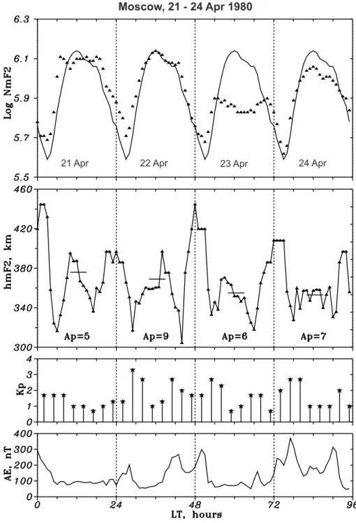
During the equinoctial transitions, large deviations of foF2 from the monthly median occur as will be explained in the following. The deviations can be positive or negative with respect to the monthly median and they are not related to ge-omagnetic activity as usual F2-layer storms. Two such ex-amples observed at Moscow on 29 Sep 1980 and 23 Apr 1980 are shown in Figs. 2 and 3. Daily Ap, 3-hour Kp, and hourly AE indices are given as well. According to com-monly accepted classification, both periods can be
consid-Table 4. Start and end dates and durations averaged over all stations
of the equinoctial transitions
Period Start date End date Duration, days
Solar min 18 Mar±5 14 Apr±11 27±8 14 Sep±7 06 Oct±5 22±6
Solar max 26 Mar±5 16 Apr±7 21±6 16 Sep±7 03 Oct±4 17±5 All years 21 Mar±6 15 Apr±9 25±7 15 Sep±7 05 Oct±4 20±5
ered as magnetically quiet. Nevertheless the day-time NmF2 deviations are very distinct – a factor of 2 in both cases. Vari-ations of the F2-layer maximum height, hmF2, calculated from theM(3000)F2 parameter using the Bradley-Dudeney (1973) expression, are given in Figs. 2 and 3 as well. Al-though the absolute accuracy of such an hmF2 determina-tion may be not very high, relative (daily) variadetermina-tions can be considered as reliable. Average day-time F2-layer heights are indicated in Figs. 2 and 3 as thin lines. Some day-to-day hmF2 variations can be seen but these differences in the average hmF2 may be not meaningful keeping in mind the large fluctuations of the hourly hmF2 values. The most in-teresting result is a relatively small daily hmF2 change while the NmF2 day-to-day variations are large. This peculiarity of NmF2 and hmF2 daily variations is discussed later using IS observations. It should be stressed that such NmF2 and hmF2 behavior is never observed at midlatitudes during F2-layer storms resulting from geomagnetic disturbances.
Moscow, 27 - 30 Sep 1980
27 Sep 28 Sep 29 Sep 30 Sep
Fig. 2. An example of strong pos-itive quiet-time NmF2 deviations ob-served at Moscow in September 1980. Monthly median NmF2 is shown as solid line (top panel). Diurnal varia-tions of hmF2 inferred from M(3000)F2 parameter are shown in the second panel. Averages of hmF2 from 10–15 LT are shown as horizontal thin lines. Daily Ap, 3-hour Kp and hourly AE in-dices are shown in the third and fourth panels.
and St. Petersburg (1960–1989) have been analyzed. Aver-aged foF2 values for 12–14 LT were compared with monthly medians and cases with large (more than 40% in NmF2) de-viations were considered for quiet (Ap≤12 for the day and the previous day) periods. The annual distribution of these deviations is given in Fig. 4 for the two stations. Both nega-tive and posinega-tive deviations (as well as their sum) show well-pronounced maxima around the equinoxes, manifesting the equinoctial transitions in the F2-region. Such quiet-time and relatively strong (NmF2obs/NmF2med≥40%) deviations are not numerous (see Fig. 4). The most abundant occurred in 1960 (12/0), 1967 (5/15), 1969 (11/10), 1970 (8/15), 1974
(12/0) where the digits in brackets give the number of posi-tive/negative deviations. The frequency of positive and nega-tive deviations varies from year to year but no regularity has been revealed yet. There are years (1960, 1973, 1974) when only positive deviations took place while negative ones pre-vailed in 1962, 1967, 1970.
Moscow, 21 - 24 Apr 1980
21 Apr 22 Apr 23 Apr 24 Apr
Fig. 3. Same as Fig. 2 but for a strong
negative quiet time NmF2 deviation ob-served at Moscow on 23 Apr 1980.
and 3). The number of available observations is not sufficient especially in the western hemisphere to draw a confident con-clusion, nevertheless, the main feature of these variations is clearly seen in the European sector where the number of ob-servations is sufficient (Fig. 5). In both cases this looks like a wave with a steep front where both maximum and mini-mumRvalues are located in a narrow longitudinal interval. This behavior is similar to the springtime transition in atomic oxygen reported by Shepherd et al. (1999) who suggested a wave-like emission rate enhancement traveling westward. An additional analysis of cases similar to 29 Sep and 23 Apr 1980 (Figs. 2 and 3) is required to consider the longitudinal
dynamics of such deviations.
Latitudinal variations ofRin the European sector for the two days 29 Sep 1980 and 2 Apr 1992 (discussed later) with positive NmF2 deviations are shown in Fig. 6. A well-pro-nounced latitudinal dependence is clearly seen in both cases with the amplitude of the NmF2 deviation increasing with latitude.
4 Incoherent scatter data analysis
Moscow (1958-1988) St. Petersburg (1960-1989)
1 2 3 4 5 6 7 8 9 10 11 12
Months 0 10 20 30 40 50 N u m b er of cas es
Deviatons of both signs
1 2 3 4 5 6 7 8 9 10 11 12
Months 0 10 20 30 40 50 60 70 80 N u m b er of cas es
Deviations of both signs
1 2 3 4 5 6 7 8 9 10 11 12
Months 0 5 10 15 20 25 Num b e r o f ca se s Negative deviations
1 2 3 4 5 6 7 8 9 10 11 12
Months 0 5 10 15 20 25 N u m b er of cas es Negative deviations
1 2 3 4 5 6 7 8 9 10 11 12
Months 0 5 10 15 20 25 30 35 N u m b er of cas es Positive deviations
1 2 3 4 5 6 7 8 9 10 11 12
Months 0 10 20 30 40 50 60 N u m b er of cas es Positive deviations
Fig. 4. Annual distribution of strong
quiet-time (Ap ≤ 12) deviations at Moscow and St. Petersburg for a 30-year period. Histograms for positive, negative deviations as well as for their sum are given separately.“Strong” was defined as a NmF2 deviation >40% from monthly median. Note the annual peaks clustering around equinoxes.
changes during the equinoctial transitions. A method devel-oped by Mikhailov and Schlegel (1997), with later modifica-tions (Mikhailov and F¨orster, 1999; Mikhailov and Schlegel, 2000), applied to Millstone Hill and EISCAT observations enables us to find thermospheric neutral composition, tem-perature and vertical plasma drift related to the meridional neutral winds. The details of the method may be found in the above references; therefore only the main idea is sketched here. The standard set of IS observations (Ne(h), Te(h), Ti(h), Vz(h) profiles) is the initial input information. All these observed parameters are contained in the continuity equations for the main ionospheric ions in the F2-region. By fitting the calculatedNe(h)profile to the experimental one, the set of main aeronomic parameters responsible for the ob-servedNe(h)distribution can be found. The most important parameters are: neutral composition (O, O2, N2), tempera-tureTn(h), total EUV solar flux, ion-molecular (O++N2)
reaction rate constant and vertical plasma drift W, result-ing from the thermospheric winds and electric fields.Neutral composition, temperature and winds are the most variable parameters and they are our main concern in this study. The other important parameters such as total EUV solar flux or O++N2reaction rate coefficient may be specified once and for all as in our previous analysis (Mikhailov and Schlegel, 2000).
Table 5. Aeronomic parameters calculated for 300 km height and 12 LT at Millstone Hill for winter and summer days. MSIS-83 model
values (second line) are given for comparison
Date Tex log[O] log[O2] log[N2] O/N2 q/103 β/10−4 W
(K) (cm−3) (cm−3) (cm−3) (cm−3s−1) (s−1) (m/s)
12 Jan 1990 1142 8.916 6.828 8.218 4.99 1.04 1.81 –10.7 logNmF2 = 6.34 1183 9.023 7.084 8.472 3.56
hmF2 = 282 km
26 Jun 1990 1234 8.708 6.959 8.474 1.71 0.66 3.05 –1.2 logNmF2 = 5.77 1309 8.826 7.082 8.541 1.93
hmF2 = 290 km
hmF2 values are higher than winter ones but the difference is not so large due to a higher solar activity level for the win-ter day. Seasonal variation of thermospheric winds and re-lated neutral composition changes are crucial for understand-ing the observed seasonal difference in the F2-layer param-eters (Ivanov-Kholodny and Mikhailov, 1986). The calcu-lation procedure of Mikhailov and Schlegel (1997) uses ob-served smoothed day-time profiles. Due to infrequent mea-surements at Millstone Hill (three per hour) available for the analyzed periods, median Ne(h), Te(h), Ti(h), Vz(h) pro-files were calculated over a 2.5–3.0 hour time interval cen-tered around 12 LT and these height profiles were used in our calculations. The derived aeronomic parameters for the two days are given in Table 5 together with F2-layer maximum parameters read from the smoothedNe(h)profiles.
The main difference between the winter and summer ther-mosphere is a decreased atomic oxygen concentration in summer (despite higher neutral temperature) and increased concentrations of molecular species. Low [O] results in lower ion production rateqin summer while increased [N2], [O2] and temperature result in larger summer linear loss co-efficientβ (Table 5). Such variations of neutral composition and temperature result, therefore, in lower summer NmF2 values compared to winter ones. This is a well-known F2-layer seasonal anomaly (Yonezawa and Arima, 1959; Rish-beth and Setty, 1961; Torr and Torr, 1973) analyzed in detail by Ivanov-Kholodny and Mikhailov (1986). Another win-ter/summer difference is in vertical plasma drift,W, which, at midlatitudes and during quiet conditions, is mainly due to thermospheric winds. The calculated winter plasma drift corresponds to a moderate (49 m/s) northward wind along the magnetic meridian while the corresponding summer merid-ional wind is close to zero. This is in line with the re-sults of a recent wind analysis at Millstone Hill (Buonsanto and Witasse, 1999). Therefore, the winter-type F2-layer pa-rameter variations is characterized by increased atomic oxy-gen concentration and northward thermospheric wind during day-time hours. On the contrary, low [O] and small merid-ional wind characterize the summer conditions. These fea-tures are important for further analysis. Increased molecular species N2 and O2concentrations in the summer F2-region are mainly due to higher neutral temperature (Table 5).
29 Sep 1980
23 Apr 1980
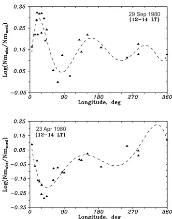
Fig. 5. Longitudinal variation for the amplitude of strong quiet-time
NmF2 deviations observed in the European sector on 29 Sep 1980 (positive deviation) and 23 Apr 1980 (negative deviation). Northern hemisphere ionosonde stations located in the 50±5◦latitudinal cor-ridor are used in the analysis. The dashed line represents a polyno-mial (the 5thorder) least squares approximation. Note that maximal and minimal deviations are located in a narrow longitudinal sector.
Table 6. Calculated thermospheric parameters at Millstone Hill
compared with MSIS-83 model predictions (second line) at 300 km. Tex values, derived with an algorithm used at Millstone Hill, are given in the third line
Date Tex log[O] log[O2] log[N2] W
(K) (cm−3) (cm−3) (cm−3) (m/s)
22 Sep 1998 1022 8.853 6.633 8.055 –6.5 logNmF2 = 5.98 1132 8.875 6.907 8.284
hmF2 = 284 km 1060
23 Sep 1998 1074 8.657 6.607 8.066 +0.2 logNmF2 = 5.83 1160 8.885 6.960 8.321
hmF2 = 290 km 1130
Millstone Hill observations in September 1998 is shown in Fig. 8. The top panel of Fig. 8 gives foF2 variations for 6 con-secutive days, while the bottom part shows diurnal variations of NmF2 and hmF2 for two days analyzed with our method. A winter-like (WS) type of the foF2 variation on 22 Sep is followed by a summer (S) one on 23 Sep , both days being magnetically quiet. It is interesting to note that the next day, 24 Sep, was magnetically moderately disturbed (Ap = 28) but the day-time foF2 values were larger than on 23 Sep. A very disturbed day, 25 Sep with low foF2, is followed by a moderately disturbed 26 Sep with a well-pronounced winter-type (WW) foF2 diurnal variation. In this case, as mentioned earlier, geomagnetic storms seem to stimulate the transition to the other type of diurnal foF2 variation. While day-time NmF2 values on 22 Sep are greater than on 23 Sep, the hmF2 values are slightly lower. In general, 22 Sep/23 Sep can be regarded as belonging to the analyzed class of events. On one hand they demonstrate the winter/summer transition; on the other hand, 23 Sep may be considered as an example of a quiet-time negative foF2 deviation.
Calculated thermospheric parameters, for the two days at 18 UT (13 LT), are given in Table 6. The most important re-sult is a 57% decrease in atomic oxygen concentration on 23 Sep with respect to 22 Sep, the concentration of molecular species being practically unchanged. The calculated verti-cal plasma drift,W, is also different for the two days cor-responding to a northward meridional wind on 22 Sep and being close to zero on 23 Sep. The 57% decrease in [O] at 300 km corresponds to a depletion of the total atomic oxygen abundance as neutral temperature and neutral scale height are larger on 23 Sep. ThisTex increase is seen in our calcula-tions, in the values derived at Millstone Hill with a different algorithm (Buonsanto and Pohlman, 1998), as well as in the MSIS-83 model predictions. The latter however, just reflect a small increase in Ap index on 23 Sep (Ap=11) compared to 22 Sep (Ap=7). Therefore, the selected two days 22 Sep/23 Sep demonstrate thermospheric parameter variations which are typical for WW and SS days, analyzed earlier. The only difference is a small change in molecular species concentra-tions.
A similar analysis was performed using EISCAT
observa-29 Sep 1980
02 Apr 1992
Fig. 6. Latitudinal variation for the amplitude of quiet-time positive
NmF2 deviations observed in the European sector on 29 Sep 1980 and 02 Apr 1992. Mostly European ionosonde stations are used to derive the figures.
12 Jan 1990 26 Jun 1990
12 Jan 1990 26 Jun 1990
Fig. 7. Diurnal variations of NmF2 and hmF2 observed at Millstone Hill for winter and summer conditions during solar maximum. The selected days il-lustrate well-pronounced winter (WW) and summer (SS) types of diurnal vari-ations.
Table 7. Calculated thermospheric parameters at EISCAT
com-pared with MSIS-83 model predictions (second line) at 300 km
Date Tex log[O] log[O2] log[N2] W
(K) (cm−3) (cm−3) (cm−3) (m/s)
01 Apr 1992 1241 8.798 6.956 8.412 +1.6 logNmF2 = 5.89 1337 8.836 7.214 8.506 hmF2 = 301 km
02 Apr 1992 1265 8.984 7.026 8.429 –10.5 logNmF2 = 6.11 1269 8.883 7.089 8.435 hmF2 = 309 km
Therefore, the chosen two days also belong to the same class of analyzed events. 02 Apr 1992 represents a good example of a quiet time F2-layer deviation. The results of the ther-mospheric parameter calculations for the two days at 13 UT (around 14 LT) are given in Table 7.
Analogous to the 22/23 Sep 1998 case, the calculations show a 53% increase in [O] on 02 Apr with respect to 01 Apr, the concentration of molecular species being practically unchanged. The vertical plasma drift,W, is also different for the two days, corresponding to a northward meridional wind of 48 m/s on 02 Apr and to a small equatorward wind of 7.4 m/s on 01 Apr. The conversion ofW to meridional wind is justified at the EISCAT location where the magnetic declination is small(D=1.24◦)and the contribution of the zonal thermospheric wind component toW is not essential.
We can conclude that, in the results of both incoherent scatter observations (Millstone Hill and EISCAT), the ob-served quiet-time NmF2 deviations are entirely due to the atomic oxygen variation in the thermosphere. The changes of the linear loss coefficientβ =k1[N2] +k2[O2]are small (due to small [O2], [N2] and reaction rate constants k1, k2 variations) and the relative solar EUV flux variations are also small for the neighbouring days. Small hmF2 daily varia-tions are due to negligible changes inβwhile the effects of
changes in [O] andW on this quantity are mostly compen-sated as they work in opposite directions (see later).
5 Discussion
Seasonal changes of neutral composition in the thermosphere are due to seasonal variations in global thermospheric circu-lation, according to present understanding confirmed by 3D model calculations (e.g. Rishbeth and M¨uller-Wodarg, 1999, and references therein). Summer-to-winter flow of air, di-rected downwards at subauroral latitudes, enriches the win-ter hemisphere with atomic oxygen while upward flow in the summer hemisphere decreases the atomic oxygen abun-dance. In accordance with this concept and with thermo-spheric wind observations (Wickwar, 1989; Buonsanto and Witasse, 1999) strong poleward wind prevails during all day-time hours in winter, while in summer the meridional wind velocity is much smaller with a direction change from pole-ward to equatorpole-ward soon after 12 LT. Our calculations for days with winter and summer-type diurnal NmF2 variations reproduce such seasonal changes both in day-time thermo-spheric wind velocity and in atomic oxygen abundance; i.e. days with winter-type diurnal NmF2 variation correspond to strong poleward wind and high [O] while summer-type NmF2 variation corresponds to small (close to zero around 12–14 LT) meridional wind and low atomic oxygen concen-tration.
21 Sep 22 Sep 23 Sep 24 Sep 25 Sep 26 Sep
22 Sep 1998 23 Sep 1998
22 Sep 1998 23 Sep 1998
Fig. 8. Daily foF2 variation for
suc-cessive days during an autumnal transi-tion period at Millstone Hill (top panel). Daily Ap indices are given as well. Bot-tom panels show diurnal NmF2 and hmF2 variations for a winter-like (22 Sep 1998) and summer-like (23 Sep 1998) day analyzed for thermospheric parameter variations (LT=UT−5).
coefficientβ is 68% larger due to higher temperature and molecular species concentrations. Lowq and largeβ result in low summer NmF2. This is the well-known explanation of the F2-layer seasonal anomaly.
The role of vibrationally excited N∗2in reducing summer NmF2 is also discussed in the literature (Pavlov, 1986; Ennis et al., 1995; Pavlov et al., 1999, and references therein). In accordance with the results of our previous analysis (Mikhai-lov and Schlegel, 2000) we use, in our model calculations, recent laboratory measurements of the O++N2reaction rate constant (Hierl et al., 1997) which takes the vibrationally ex-cited N∗2 into account. For the night, there is no seasonal F2-region anomaly; i.e. night-time summer NmF2 values are higher than the corresponding winter values. This re-sults in a seasonal difference of NmF2max/NmF2min, as ob-served. This effect is not related to seasonal variations of neutral composition but is due to a different diurnal variation of thermospheric winds during winter and summer (Ivanov-Kholodny and Mikhailov, 1986).
During the transition, we never observed, on adjacent days, such strong diurnal NmF2 variations as those shown in Fig. 7 for the completely developed WW- and SS-types on 12 Jan and 26 Jun 1990. Nevertheless, two distinctive features – a
31 Mar 01 Apr 02 Apr 03 Apr
01 Apr 1992 02 Apr 1992
01 Apr 1992 02 Apr 1992
Fig. 9. Daily foF2 variation for
suc-cessive days during a vernal transition period at EISCAT (top panel). Daily Ap indices are also given. Bottom pan-els show diurnal NmF2 and hmF2 vari-ations for a winter-like (02 Apr 1992) and summer-like (01 Apr 1992) day analyzed for thermospheric parameter variations (LT=UT−1.3).
Shepherd et al. (1999) observed large variations of atomic oxygen concentration in the lower E region and related these to vertical air motions. Downward mass motion increases the atomic oxygen abundance while upward motion depletes the thermospheric [O] abundance. Using Millstone Hill IS ob-servations it was shown by Ivanov-Kholodny et al. (1981) that day-to-day NmF2 and hmF2 variations are in phase in summer and that they are accompanied by similar variations in foE. The effect of simultaneous changes of electron con-centration in the ionospheric E and F2-regions was also theo-retically modeled by Mikhailov (1983) who showed that such variations can be explained by day-to-day changes in verti-cal mass velocity of about 1–2 cm s−1 at E-region heights, resulting in [O] and [O2] anti-phase changes. The results of those model calculations yielded day-to-day variations at 300 km for neighbouring days of 1log[O] ≈ 0.2(58%), 1log[O2] ≈ 0.08(20%), and1log[N2] ≈ 0.01. The lat-ter results in very small changes of the linear loss coefficient β. Such variations of [O] andβagree with the results of our present calculations of the thermospheric parameter changes for 22 Sep/23 Sep 1998 and 01 Apr/02 Apr 1992 (Tables 6 and 7).
It should be noted that in our model is no provision to
for instance, by ESRO-4 (Pr¨olss, 1982) and by DE-2 (Burns and Killeen, 1992).
An analysis of WINDII observations of the oxygen green line emission rate by Ward et al. (1997) revealed vertical motions associated with a quasi-two day wave at E-region heights. Mean vertical winds of a few cm s−1have been de-duced from the WINDII data by Fauliot et al. (1997). Sim-ilarly, ground-based radar observations by Voiculescu et al. (1999) proved a strong influence of the planetary quasi 2-day wave on the mid-latitude E region. At F2-region heights, quasi 2-day oscillations in NmF2 are widely discussed in the literature (e.g. Apostolov et al., 1995; Forbes et al., 1997 and references therein). Unfortunately, Millstone Hill obser-vations are not available at E-region heights for the analyzed period 22/23 Sep 1998 and particle precipitation perturbs the auroral E-region (EISCAT location) even during rather quiet time periods. Therefore, it was not possible to check the pres-ence of simultaneous electron density changes in E and F2 regions for the two periods in question. But such an analysis is possible with mid-latitude ground-based ionosonde obser-vations as performed by Mikhailov (1983).
The quiet-time NmF2 deviations during the transition pe-riods and its seasonal (Fig. 4) and spatial (Figs. 5 and 6) dependencies have been described in detail in Sect. 3. On the one hand, such strong NmF2 deviations, of up to a fac-tor of 2 as on 29 Sep and 23 Apr 1980 (Figs. 2 and 3), are comparable with F2-layer storm effects related to strong geo-magnetic disturbances but their mechanism is different from usual F2-layer storm effects outlined above. On the other hand, the spatial variations of their amplitude may tell us about longitudinal and latitudinal variations of the thermo-spheric circulation pattern during the transition periods. The effect may be related to quasi 2-day oscillations occurring mainly during summer but with maximum amplitudes dur-ing equinoxes (Forbes et al., 1992). Indeed, Fig. 4 shows that strong quiet time NmF2 deviations are most probable around equinoxes. A well-pronounced wave-like longitudi-nal structure of such deviations (Fig. 5), with maxima and minima located in rather narrow longitudinal sectors, ob-viously reflects the corresponding longitudinal structure in thermospheric winds during the transition periods. Obvi-ously, the revealed effect of the quiet-time F2-region devia-tions needs further analysis using the world-wide ionosonde network together with IS and optical observations.
6 Conclusions
The main results of our analysis can be summarized as fol-lows:
1. The transitions from winter to summer-type diurnal foF2 variation, averaged for 6 stations and years of solar maximum and minimum, occur during 20–25 days; the ver-nal transition lasts a little longer than the autumver-nal one. The vernal transition starts close to the equinox while the autum-nal one starts earlier. Both transitions start a little earlier dur-ing solar minimum and last longer compared to solar
max-imum. This may be due to stronger thermospheric winds and less inertia of the thermosphere during solar minimum. Cases of very fast (6–10 days) transitions are revealed at par-ticular stations. Neither latitudinal nor longitudinal varia-tions, for the dates and duration of the transivaria-tions, could be derived within the available accuracy of these parameters.
2. Strong (up to a factor of 2) day-time NmF2 devia-tions of both signs, not related to geomagnetic activity, are revealed for the transitions. Both negative and positive de-viations cluster around equinoxes suggesting a relationship with the equinoctial transitions in the F2–region. The actual number of positive and negative deviations varies from year to year but no regularity has been found. There are years (1960, 1973, 1974) when only positive deviations took place but negative deviations prevailed in 1962, 1967, 1970.
3. The longitudinal variation pattern of such quiet-time NmF2 deviations resembles a wave with a steep front since both maximum and minimum NmF2obs/NmF2medvalues are located in a narrow longitudinal interval. A well-pronounced latitudinal increase of the amplitude of the NmF2 deviation was observed for cases of positive NmF2 deviations. No lati-tudinal dependence was found for negative NmF2 deviations. 4. Estimates of thermospheric parameters, using EIS-CAT and Millstone Hill IS observations for adjacent days during the transition periods with different type of diurnal NmF2 variations, have shown that summer-like days are dis-tinguished by decreased (by ≈ 55%) atomic oxygen con-centration compared to winter-like days, molecular N2 and O2concentrations being almost unchanged day-time merid-ional thermospheric wind (inferred from vertical plasma drift W) is small and equatorward for summer-like days unlike the strong northward winds for winter-like days. Therefore, the observed quiet-time NmF2 deviations are entirely due to the atomic oxygen variation in the thermosphere as the lin-ear loss coefficientβ=k1[N2] +k2[O2]variations are small (due to small [O2], [N2] and reaction rate constants k1, k2 variations). Relative solar EUV flux variations are also small for the adjacent days. Small hmF2 day-to-day variations are due to negligible variation inβ while the effects of [O] and Wchanges are compensated to a large extent as they work in opposite directions.
pro-viding the data. The EISCAT Scientific Association is funded by scientific agencies of Finland (SA), France (CNRC), Germany (MPG), Japan (NIPR), Norway (NF), Sweden (NFR) and the United Kingdom (PPARC). This work was supported under NATO grant EST.EV.976711.
Topical Editor M. Lester thanks A. C. Schlesier and another ref-eree for their help in evaluating this paper.
References
Apostolov, E. M., Altadill, D., and Alberca, L., Characteristics of quasi-2-day oscillations in the foF2 at northern middle latitudes, J. Geophys. Res., 100, 12163–12171, 1995.
Bradley, P. A. and Dudeney, J. R., A simple model of the vertical distribution of electron concentration in the ionosphere, J. At-mos. Terr. Phys., 35, 2131–2146, 1973.
Buonsanto, M. J. and Pohlman, L. M., Climatology of neutral exo-spheric temperature above Millstone Hill, J. Geophys. Res., 103, 23381–23392, 1998.
Buonsanto, M. J. and Witasse, O. G., An update climatology of ther-mospheric neutral winds and F region ion drifts above Millstone Hill, J. Geophys. Res., 104, 24675–24687, 1999.
Burns, A. G. and Killeen, T. L., The equatorial neutral thermo-spheric response to geomagnetic forcing, Geophys. Res. Lett., 19, 977–980, 1992.
Ennis, A. E., Bailey, G. J., and Moffett, R. J., Vibrational nitrogen concentration in the ionosphere and its dependence on season and solar cycle, Ann. Geophysicae, 13, 1164–1171, 1995. Evans, J. V., Millstone-Hill Thomson scatter results for 1965,
Planet. Space Sci, 18, 1225–1252, 1970.
Evans, J. V., Millstone-Hill Thomson scatter results for 1966 and 1967, Planet. Space Sci., 21, 763–792, 1973.
Evans, J. V., Millstone-Hill Thomson scatter results for 1969, Lin-coln Lab., M.I.I., Lexington, Mass. Tech. Rep., N 513, 1974. Forbes, J. M., Guffee, R., Zhang, X., Fritts, D., Riggin, D., Manson,
A., Meek, C., and Vincent, R. A., Quasi 2-day oscillation of the ionosphere during summer 1992, J. Geophys. Res., 102, 7301– 7305, 1997.
Fauliot, V., Thuillier, G., and Vial, F., Mean vertical wind in the mesosphere-lower thermosphere region (80–120 km) deduced from the WINDII observations on board UARS, Ann. Geophys-icae, 15, 1221–1231, 1997.
Fuller-Rowell, T. J. and Rees, D., Derivation of a conservation equa-tion for mean molecular weight for a two-constituent gas within a three-dimensional, time-dependent model of the thermosphere, Planet. Space Sci., 31, 1209–1222, 1983.
Hierl, P. M., Dotan, I., Seeley, J. V., Van Doran, J. M., Morris, R. A., and Viggiano, A. A., Rate coefficients for the reactions of O+with N2and O2as a function of temperature (300–188 K), J. Chem. Phys., 106 (9), 3540–3544, 1997.
Ivanov-Kholodny, G. S., Mikhailov, A. V., and Ostrovskiy, G. I., Day-to-day change in the summer values of hmF2 and NmF2 as a reflection of variations in the neutral composition of the upper atmosphere, Geomagn. Aeronom., 21, 615–617, 1981.
Ivanov-Kholodny, G. S. and Mikhailov, A. V., The prediction of ionospheric conditions, D. Reidel Publ. Co., Dordrecht, Holland, 1986.
Mikhailov, A. V., Possible mechanism for the in-phase changes in the electron densities in the ionospheric E and F2 regions, Geo-magn. Aeronom., 23, 455–458, 1983.
Mikhailov, A. V. and F¨orster, M., Some F2-layer effects during the 06–11 January 1997 CEDAR storm period as observed with the Millstone Hill incoherent scatter facility, J. Atmos. Solar-Terr. Phys., 61, 249–261, 1999.
Mikhailov, A. V. and Schlegel, K., Self-consistent modeling of the day-time electron density profile in the ionospheric F-region, Ann. Geophysicae, 15, 314–326, 1997.
Mikhailov, A. V. and Schlegel, K., A self-consistent estimate of O++N2rate coefficient and total EUV solar flux withλ <1050
˚
A using EISCAT observations, Ann. Geophysicae, 18, 1164– 1171, 2000.
Pavlov, A. V., Rate coefficient of O+with vibrationally excited N2 in the ionosphere, Geomag. i Aeronom., 26, 166–168, 1986 (in Russian).
Pavlov, A. V., Buonsanto, M. J., Schlesier, A. C., and Richards, P. G., Comparison of models and data at Millstone Hill during the 5–11 June 1991 storm, J. Atmos. Solar-Terr. Phys., 61, 263–279, 1999.
Pr¨olss, Perturbation of the low-latitude upper atmosphere during magnetic substorm activity, J. Geophys. Res., 87, 5260–5266, 1982.
Rishbeth, H. and Setty, C. S. G. K., The F-layer at sunrise, J. Atmos. Terr. Phys., 21, 263–276, 1961.
Rishbeth, H. and M¨uller-Wodarg, I. C. F., Vertical circulation and thermospheric composition: a modelling study, Ann. Geophysi-cae, 17, 794–805, 1999.
Shepherd, G. G., Stegman, J., Espy, P., McLandress, C., Thuillier, G., and Wiens, R. H., Springtime transition in lower thermo-spheric atomic oxygen, J. Geophys. Res., 104, 213–223, 1999. Torr, M. R. and Torr, D. G., The seasonal behavior of the F2-layer
of the ionosphere, J. Atmos. Terr. Phys., 35, 2237–2251, 1973. Voiculescu, M., Haldoupis, C., and Schlegel, K., Evidence for
plan-etary wave effects on midlatitude backscatter and sporadic E layer occurrence, Geophys. Res. Lett., 26, 1105–1108, 1999. Ward, W. E, Solheim, B. H., and Shepher, G. G., Two day wave
induced variations in the oxygen green line volume emission rate: WINDII observations, Geophys. Res. Lett., 24, 1227–1130, 1997.
Wickwar, V. B., Global thermospheric studies of neutral dynam-ics using incoherent scatter radars, Adv. Space Res., 9, 87–102, 1989.
Yonezawa, T., On the seasonal and non-seasonal annual variations and the semi-annual variation in the noon and midnight electron density of the F2layer in middle latitudes, J. Radio Res. Labs., 6, 651–668, 1959.