On the Reliability of Consecutive Systems

On the Reliability of Consecutive Systems

Spiros D. Dafnis, Frosso S. Makri and Zaharias M. Psillakis

Abstract_{—A consecutive system, the failure of}

which depends on the occurrence of a number of failure-success patterns, is introduced. It extends several consecutive systems studied so far in the lit-erature. The exact system reliability is determined for systems with independently functioning compo-nents. The derivations are based on the exact dis-tribution of properly defined random variables whose distributions are obtained by employing an appropri-ate Markov chain imbedding technique. The results are illustrated by numerical examples.

Keywords: consecutive systems, reliability, Markov chain imbedding

1

Introduction

A consecutive-k-out-of-n:F system, denoted as C(k, n : F), consists of an ordered sequence of ncomponents for which the existence of k (or more) consecutive failed components causes the system’s failure, 1 ≤ k ≤ n. C(1, n : F) and C(n, n : F) are series and parallel sys-tems with ncomponents, respectively. Since Kontoleon [12] first introduced and studied these systems in 1980, a series of articles have been published studying their reliability properties under various assumptions because of their wide applicability; e.g. they have been used to model telecommunication systems, oil pipeline systems, vacuum accelerators, etc. For extensive reviews of such systems and the used methods to evaluate their reliabil-ity under several component dependencies, we refer to [3], [13] and [19]. For recent contribution on the subject see e.g. [4], [5], [17] and the references therein.

However, a situation may occur in which the system does not weaken so as to fail because of the existence of a run of kconsecutive failed components, if this failure run is fol-lowed by a run of consecutive working components with sufficiently large length. That is, we consider a system that fails if there are k1 consecutive failed components,

k1 ≥k, followed by less thank1+r, r≥0, consecutive working ones. We call such a system consecutive-k, r -out-of-n:FS system and we denote it as C(k, r, n : F S). Givennandk, 1≤k≤n: (a)C(k, r, n:F S) reduces to

C(k, n:F) for n <2k,r≥0 or for anyr > n−2k≥0; and (b) for 0 ≤ r ≤ n−2k, C(k, r, n : F S) is a new system more reliable than C(k, n: F) with the same k andn. This is so because the set of possible state config-urations causingC(k, r, n:F S) failure is a subset of the respective set of aC(k, n:F).

To understand these systems consider one possible string SF F F SSSSSS forn= 10,k= 2,r= 2, where the sym-bols S, F denote functioning, failed component states, respectively. In this case, since there are 3 (at least two) consecutive failures a C(2,10 : F) fails but, since the 3 consecutive failed components are followed by 6 (at least 3+2) working components aC(2,2,10 :F S) system does not fail. However, SF F F SSF SSS represents a failure state of both types of systems.

A generalization of a consecutive-k-out-of-n:F system was formulated by Griffith [9], who considered a system of n (n ≥ mk) components ordered on a line, for which m (≥ 2) non-overlapping strings of k consecutive failed components are needed for system failure. For such a sys-tem, named m-consecutive-k-out-of-n:F system and de-noted as Cm(k, n:F), in [16] and [1] exact formulae for its reliability, when the components of the system are iid (independent and identically distributed), have been given. In [18] the failure probability ofCm(k, n:F) hav-ing independent components was obtained while in [8] the Stein-Chen method was employed to obtain Poisson approximations for the reliability.

Following the idea of this generalization Agarwal et al. [1] argued that a situation may arise in which a system fails if there are at least m non-overlapping runs of at least k consecutive failures. They called such a system m-consecutive-at least-k-out-of-n:F and they employed GERT analysis to obtain the reliability of the system when its components are iid. This system, was denoted as Cm+(k, n: F) and for m = 1 reduces to C(k, n : F). It is mentioned that for Cm+(k, n : F) a run of failures of length rk, r ≥ 1, is treated as one run of length at least k whereas it is treated as r runs of length k for a Cm(k, n:F).

∗_{Date of the manuscript submission: 10/01/10. Corresponding author: Spiros D. Dafnis. First author address: Department of}

Extending the above generalization we consider a sys-tem ofncomponents ordered on a line that fails if there are at least m (m ≥ 1) runs of failed components of lengths ki (ki ≥ k), i = 1, . . . , m, . . ., such that the

i-th failure run (of length ki) is followed by less than

ki+r working components, r ≥0, 1≤k ≤n. We call such a systemm-consecutive-k,r-out-of-n:FS system and we denote it as Cm(k, r, n : F S). This system reduces to anm-consecutive-at least-k-out-of-n:F system for any r > n−2k≥0 and obviously forn <2k,r≥0. Readily, for a fixedm≥1,Cm(k, r, n:F S) with 0≤r≤n−2k, is more reliable thanCm+(k, n:F) which in turns is more re-liable thanCm(k, n:F) with the same parameterskand

n. These are true, because the set of possible state config-urations causingCm(k, r, n:F S) failure is a subset of the set of possible state configurations causing Cm+(k, n:F) failure which in turns is a subset of the respective set of a Cm(k, n:F). For the following sequence ofn= 15 trials

F F SSSSSF F F SSSSS a C₂+(2,15 : F) fails whereas a C2(2,2,15 :F S) functions.

In this paper we employ an appropriate Markov chain imbedding technique to obtain the reliabilities of an m-consecutive-at least-k-out-of-n:F (m ≥ 1), a consecutive-k, r-out-of-n:FS system and the generalized m-consecutive-k, r-out-of-n:FS (m≥2), when the system components are independently functioning with not nec-essarily equal reliabilities, via the determination of the exact distribution of properly defined random variables (RVs). The theoretical results are clarified further by nu-merical examples. Specifically, the study is organized as follows.

In Section 2.1 we establish the reliability of a general class of consecutive systems along with a brief discussion of the Markov chain imbedding method for enumerating RVs. In Section 2.2 we derived the reliability of the under study systems which are presented in Theorems 1 and 2. Finally, in Section 3 we highlight a potential use of such systems in applied research.

2

Reliability of consecutive systems

The reliability of any consecutive system mentioned in Section 1 can be formulated using the following general setup.

2.1

Preliminaries and general results

Let a system consist of an ordered (linear) sequence ofn (n > 0) components. Each component and the system itself is either good (working or functioning or in state 1) or not-good (failed or no-functioning or in state 0). Let the indicator RVs Z1, Z2, . . . , Zn represent the states of the system components, i.e. Zi = 1 if componentiworks; 0, if componentifails. We say that the system fails or it is in state 0 if there are at least m (m >0) occurrences of a patternE. The patternE may be an un-interrupted

sequence of 0s or a pre-specified composition of 0s and 1s. If Xn(E) is an enumerating (non-negative) RV de-noting the number of occurrences of E in the sequence Z1, Z2, . . . , Zn and Γn = {Z1 = Z2 = . . . = Zn = 0}, then the system failure probability is

Qn,m(E) =P(Xn(E)≥m), if Γn∈(Xn(E)≥m) (1)

and

Qn,m(E) =P(Xn(E)≥m) +P( n Y

i=1

(1−Zi) = 1),

if Γn6∈(Xn(E)≥m); (2)

whereas the system working (functioning) probability, i.e. the system reliability is

Rn,m(E) = 1−Qn,m(E). (3)

In many cases the exact distribution of Xn(E), there-fore the system reliability Rn,m(E), may be captured by employing a Markov chain imbedding technique (MCIT) that projects the random variableXn(E) to appropriate subspaces of the state space of a properly defined Markov chain. Usually, a typical element of the state space is rep-resented by a 2-tuple (x, j). The first componentxstands for the number of occurrences of the pattern E whereas the second component j provides information about the stage of the formation of the next pattern.

It was the novel paper of Fu and Koutras [6] that es-tablished the concept of a Markov chain imbeddable RV (MV) and it popularized MCIT. After that, Koutras and Alexandrou [15] refined the method by providing a gen-eral recursive scheme for the probability distribution of a Markov chain imbeddable RV of binomial type (MVB). The concept of MVB was extended later by Han and Aki [10] who introduced a Markov chain imbeddable RV of returnable type (MVR) and also gave a general recur-sive scheme for its probability distribution. The papers [2], [11], [14] as well as the treatise [7] and the references therein present many aspects and applications of MCIT and its versions. In the sequel, a brief -but sufficient for our study, description of MCIT is given. It presents only a summary of the involved concepts and the necessary notation in order to make the article self-contained.

Definition 1. A random variable Xn (n a non-negative integer) with support {0,1, . . . , ℓn}, ℓn = max{x;P(Xn = x) > 0}, will be called Markov chain imbeddable variable if

(a) there exists a Markov chain {Yt;t≥0} defined on a state space Ω

(b) there exists a partition {Cx, x = 0,1, . . .} on Ω,

Cx={cx,0, cx,1, . . . , cx,s−1},s=|Cx|and (c) for everyx= 0,1, . . . , ℓn

Definition 2. A Markov chain imbeddable random vari-able will be called of

(a) Binomial type (MVB) if P(Yt = cy,j | Yt−1 =

cx,i) = 0, for all y 6= x, x+ 1, t ≥ 1, or equivalently

P(Yt∈Cy|Yt−1∈Cx) = 0, for ally6=x, x+ 1,

(b) Returnable type (MVR) if P(Yt = cy,j | Yt−1 =

cx,i) = 0, for ally6=x−1, x, x+ 1,t≥1, or equivalently

P(Yt∈Cy|Yt−1∈Cx) = 0, for ally6=x−1, x, x+ 1.

It is noted that for an MVB there are transitions within the same sub-state setCxand transitions from setCxto

Cx+1while in the case of an MVR there are, in addition, transitions from setCxtoCx−1, i.e. the process can also move backwards.

Next, let the one-steps×stransition matrices

At(x) = (α(t)ij(x)), Bt(x) = (βij(t)(x)), Dt(x) = (d(t)ij (x))

with

α(t)_ij (x) =P(Yt=cx,j |Yt−1=cx,i),

βij(t)(x) =P(Yt=cx+1,j |Yt−1=cx,i),

d(t)_ij(x) =P(Yt=cx−1,j |Yt−1=cx,i)

and ft(x) the probability vector associated with time t and sub-state set Cx, i.e., for 0≤t≤n,

ft(x) = (P(Yt=cx,0), P(Yt=cx,1), . . . , P(Yt=cx,s−1)).

Then, readily

P(Xn =x) =fn(x)1

′

, x= 0,1, . . . , ℓn (4)

with 1 = (1,1, . . . ,1) ∈ Rs_{. Also, the convention}

P(X0 = 0) = 1 implies that if πx is the (row) vector of initial probabilities of the Markov chain, i.e. πx =f0(x) thenπ01

′

= 1 andπx1

′

= 0,x >0.

The following Lemmas 1 and 2 provide recursive relations for the probability vectorsft(x).

Lemma 1. ([15]). For an MVB Xn the sequenceft(x),

t= 1,2, . . . , nsatisfies the recurrence relations

ft(0) =ft−1(0)At(0)

ft(x) =ft−1(x)At(x)+ft−1(x−1)Bt(x−1), 1≤x≤ℓn.

Lemma 2. ([10]). For an MVR Xn the sequenceft(x),

t= 1,2, . . . , nsatisfies the recursive relations

ft(x) =0, x <0, or x > ℓt

ft(x) = ft−1(x)At(x) +ft−1(x−1)Bt(x−1)

+ft−1(x+ 1)Dt(x+ 1), 0≤x≤ℓt.

As we can see the method requires, the proper state space Ω, its partition{Cx,0≤x≤ℓn} and the transition ma-trices,A,B andD, to be determined. Then, relation (4) along with Lemmas 1 or 2, provide the probability distri-bution of the under study RVXn. Therefore, within the framework of MCIT, what remains for the computation of the reliabilities of the under study consecutive systems, in particularCm+(k, n:F) andCm(k, r, n:F S), is: First, the definition of the failure patternsE which correspond to the respective systems (i.e. the associated RVs) and second, the determination of the proper state spaces and transition probability matrices. The first task is given next whereas the second is presented in Section 2.2.

Proposition 1. The correspondences among consecu-tive systems, patterns E causing their failures and the enumerating RVs used to evaluate the systems reliabili-ties are:

(I)Cm+(k, n:F): Let E ≡ Ek =F F . . . F | {z }

k₁≥k

, thenXn(E)≡

Gn,kdenoting the number of failure runs of length at least

kin a sequence ofnbinary (success-failure) trials ordered on a line. Its support is SGn,k ={0,1, . . . , ℓn = [

n+1 k+1]}, where by [x] we denote the greatest integer less than or equal tox.

(II) Cm(k, r, n: F S): LetE ≡ Ek,r =F F . . . F | {z }

k₁≥k

SS . . . S | {z } k₂<k₁+r ,

then Xn(E) ≡ Nn,k,r denoting the number of occur-rences of the pattern Ek,r in a sequence of n binary (success-failure) trials ordered on a line. Its support is SNn,k,r ={0,1, . . . , ℓn}, with ℓn= [

n+2

3 ], ifk= 1,r= 0; [n+1

k+1], otherwise.

We note that for n <2k, r ≥0 or for r > n−2k≥ 0, Nn,k,r counts asGn,k does since the numbers of the pat-ternsEkandEk,rcoincide, henceCm(k, r, n:F S) reduces to C+

m(k, n : F), for 1 ≤m ≤ ℓn. In general, Nn,k,r ≤

Gn,k for r≥0. Specifically, it holds: Nn,k,r ≤Gn,k for 0≤r≤n−2kandNn,k,r =Gn,k forr > n−2k≥0 or forn <2k,r≥0. As an example we consider again the binary sequence: F F SSSSSF F F SSSSS of n= 15 tri-als. Then, we have: Gn,2= 2,Nn,2,2= 0 andNn,2,r = 2 forr >11.

2.2

Systems with independent components

Letp= (p1, p2, . . . , pn). Since the system reliability is a function ofp, we denote byR+

m(k, n;p) andRm(k, r, n;p) the reliability functions of C+

m(k, n:F) and Cm(k, r, n:

F S) which are given in Theorems 1 and 2, respectively. The proofs of the theorems are provided in the Appendix A.

2.2.1 Reliability of an m-consecutive-at least-k -out-of-n:F system, n≥2

In [15] (see also [14]) it was proved that Gn,k is a MVB with

Cx={(x, j);j=−1,0,1, . . . , k−1}

and

At(x) =At=         

0 1 2 · k−1 −1

pt qt 0 _· 0 0

pt 0 qt _· 0 0

· · · ·

pt 0 0 _· qt 0

pt 0 0 _· 0 0

pt 0 0 _· 0 qt

         ,

Bt(x) =Bt=         

0 1 2 · k−1 −1

0 0 0 · 0 0

0 0 0 · 0 0

· · · ·

0 0 0 · 0 0

0 0 0 · 0 qt

0 0 0 · 0 0

         .

Theorem 1. For positive integers k, m and n the re-liability R+

m(k, n;p) of a Cm+(k, n : F) with indepen-dent components and reliability of the i-th component pi,i= 1,2, . . . , n, is given by

R+m(k, n;p) = 1− n Y

i=1

(1−pi), if n < mk+m−1

and

R+

m(k, n;p) = Pm−2

x=0 fn−1(x)(An +Bn)1

′

+fn−1(m − 1)An1

′

−ζ(1, m)Qn_i=1(1−pi), if n≥mk+m−1,

with An and Bn being the matrices given previously,

f’s are evaluated via the recursive scheme of Lemma 1 andζ(1, m) = 1 ifm >1; 0, otherwise.

Remark 1. For m = 1, Cm+(k, n : F) reduces to

C(k, n:F). Hence, its reliabilityR(k, n;p) can be com-puted via the relationship

R(k, n;p) =R1+(k, n;p) =fn−1(0)An1

′

, n≥k.

2.2.2 Reliability of an m-consecutive-k, r

-out-of-n:FS system, n≥2

The random variable Nn,k,r is an MVR (see, Appendix A.2) with

Cx= ½

{(x, j);j= 0,1,2}, if k= 1, r= 0, n= 2,3

{(x, j);j=−[n−r

2 ]−r+ 1, . . . ,−1,0,1, . . . ,[ n−r

2 ],[ n−r

2 ] + 1}, otherwise

and transition matricesA,B,D given as follows.

(a) Ifk >1 then

At(x) =At

=                     

0 1 2 · k−1 k k+ 1 · [n−r 2 ] [

n−r

2 ] + 1 −1 −2 · −k−r+ 1 · −[ n−r

2 ]−r+ 2 −[ n−r

2 ]−r+ 1

pt qt 0 · 0 0 0 · 0 0 0 0 · 0 · 0 0

pt 0 qt · 0 0 0 · 0 0 0 0 · 0 · 0 0

pt 0 0 · 0 0 0 · 0 0 0 0 · 0 · 0 0

· · · ·

pt 0 0 · 0 0 0 · 0 0 0 0 · 0 · 0 0

0 0 0 · 0 0 qt · 0 0 0 0 · pt · 0 0

0 0 0 · 0 0 0 · 0 0 0 0 · 0 · 0 0

· · · ·

0 0 0 · 0 0 0 · 0 qt 0 0 · 0 · 0 pt

pt 0 0 · 0 0 0 · 0 qt 0 0 · 0 · 0 0

0 qt 0 · 0 0 0 · 0 0 0 0 · 0 · 0 0

0 qt 0 · 0 0 0 · 0 0 pt 0 · 0 · 0 0

· · · ·

0 qt 0 · 0 0 0 · 0 0 0 0 · 0 · 0 0

· · · ·

0 qt 0 · 0 0 0 · 0 0 0 0 · 0 · 0 0

0 qt 0 · 0 0 0 · 0 0 0 0 · 0 · pt 0

                    

Bt(x) =Bt= (βij(t))(2[n−r

2 ]+r+1)×(2[ n−r

2 ]+r+1) with β

(t)

k−1,k=qt and βij(t)= 0 for (i, j)6= (k−1, k) and

Dt(x) =Dt= (d(t)ij )(2[n−r

2 ]+r+1)×(2[ n−r

2 ]+r+1) with d

(t)

(b) Ifk= 1, r >0, then

At(x) = At

= 

               

0 1 2 · [n−r 2 ] [

n−r

2 ] + 1 −1 −2 · −r −r−1 · −[ n−r

2 ]−r+ 2 −[ n−r

2 ]−r+ 1

pt 0 0 · 0 0 0 0 · 0 0 · 0 0

0 0 qt · 0 0 0 0 · pt 0 · 0 0

0 0 0 · 0 0 0 0 · 0 pt · 0 0

· · · ·

0 0 0 · 0 qt 0 0 · 0 0 · 0 pt

pt 0 0 · 0 qt 0 0 · 0 0 · 0 0

0 0 0 · 0 0 0 0 · 0 0 · 0 0

0 0 0 · 0 0 pt 0 · 0 0 · 0 0

· · · ·

0 0 0 · 0 0 0 0 · 0 0 · 0 0

0 0 0 · 0 0 0 0 · pt 0 · 0 0

· · · ·

0 0 0 · 0 0 0 0 · 0 0 · 0 0

0 0 0 · 0 0 0 0 · 0 0 · pt 0



               

Bt(x) =Bt = (βij(t))(2[n−r

2 ]+r+1)×(2[ n−r

2 ]+r+1) withβ

(t)

i1 =qt, i= 0,−1,−2, . . . ,−[n−₂r]−r+ 1,βij(t) = 0 for all the other entries and

Dt(x) =Dt= (d(t)ij )(2[n−r

2 ]+r+1)×(2[ n−r

2 ]+r+1)withd

(t)

−1,0=ptandd(t)ij = 0 for (i, j)6= (−1,0).

(c) Ifk= 1,r= 0, n >3 then

At(x) = At

= 

           

0 1 2 · [n 2] [

n

2] + 1 −1 −2 · −[ n

2] + 2 −[ n 2] + 1

pt 0 0 · 0 0 0 0 · 0 0

0 0 qt · 0 0 0 0 · 0 0

0 0 0 · 0 0 pt 0 · 0 0

· · · ·

0 0 0 · 0 qt 0 0 · 0 pt

pt 0 0 · 0 qt 0 0 · 0 0

0 0 0 · 0 0 0 0 · 0 0

0 0 0 · 0 0 pt 0 · 0 0

· · · ·

0 0 0 · 0 0 0 0 · 0 0

0 0 0 · 0 0 0 0 · pt 0



           

Bt(x) =Bt= (β (t) ij )(2[n

2]+1)×(2[ n

2]+1)withβ

(t)

i1 =qt,i= 0,−1,−2, . . . ,−[n₂] + 1,βij(t)= 0, for all the other entries and

Dt(x) =Dt= (d(t)ij )(2[n 2]+1)×(2[

n

2]+1) withd

(t)

−1,0=pt,d10(t)=pt andd(t)ij = 0, for all the other entries.

(d) Ifk= 1, r= 0, n= 2,3, then

At(x) = At = (a (t)

ij)3×3 with a(t)00 = a (t)

20 = pt, a (t) 12 =

a(t)22 =qt anda(t)ij = 0, for all the other entries,

Bt(x) = Bt = (β (t)

ij )3×3 with β01(t) = qt; β (t)

ij = 0, for (i, j)6= (0,1) and

Dt(x) = Dt = (d (t)

ij )3×3 with d(t)10 = pt, d (t) ij = 0, (i, j)6= (1,0).

In cases (a)-(d) the states in matrices B and D are la-belled as in the respective matrices A.

Theorem 2. The reliability Rm(k, r, n;p) of a

Cm(k, r, n : F S) for 0 ≤ r ≤ n−2k, with indepen-dent components and reliability of the i-th component

pi,i= 1,2, . . . , n, is given by:

(a) R1(k, r, n;p) =fn−1(0)An1

′

+fn−1(1)Dn1

′

;

(b) R2(k, r, n;p) =fn−1(0)(An+Bn)1

′

+fn−1(1)(An+

Dn)1

′

+fn−1(2)Dn1

′

−Qn_i=1(1−pi);

and form≥3,

(c) Rm(k, r, n;p) = P m−2

x=1 fn−1(x)(An +Bn +Dn)1

′

+fn−1(0)(An + Bn)1

′

+ fn−1(m − 1)(An + Dn)1

′

+

fn−1(m)Dn1

′

−Qni=1(1−pi),

where An, Bn, Dn are the matrices given above andf’s are evaluated via the recursive scheme of Lemma 2.

Remark 2. SinceCm(k, r, n:F S) reduces toCm+(k, n:

3

A note for application

In applied reliability studies we need to work with spe-cific systems. To this end, we consider possible examples ofC+

m(k, n:F) andCm(k, r, n:F S).

Example Let an alarm system of an accelerator consist of n (≥2) detectors (feelers) posed along the surface of an accelerator. The feelers (i.e. the system components) might measure the temperature or the radioactivity level of the accelerator. Their failures are likely to occur inde-pendently. The reliabilities of the detectors may be differ-ent because of the holding conditions and the operational procedures among the individual feelers or they may be identical due to economic reasons and maintenance pol-icy. We consider that such a system fails if there are at leastm (≥1) clusters of feelers that either: (I) each has at leastkconsecutive feelers failed or (II) thei-th cluster consists of ki (≥k) failed feelers and is followed by less thanki+rworking ones,r≥0 (i.e. a situation which im-plies a malfunction of the system which is not possible to be compensated). Readily, cases (I) and (II) correspond toCm+(k, n:F) andCm(k, r, n:F S), respectively.

Next, in order to evaluate the reliability of the alarm sys-tems discussed we consider some specific configurations of them. The system reliabilities are computed via The-orems 1 or 2 and they present results helpful to a practi-cally minded reader.

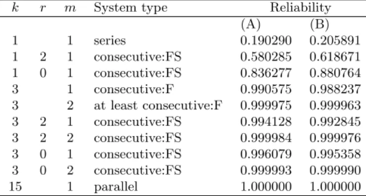
Table 1Exact reliabilities ofC+

m(k,15 :F) and

Cm(k, r,15 :F S) with independent components,

for (A)pi= 0.85 ifiis odd; 0.95, ifiis even (B)

pi=p= 0.90,i= 1,2, . . . , n

k r m System type Reliability

(A) (B)

1 1 series 0.190290 0.205891

1 2 1 consecutive:FS 0.580285 0.618671

1 0 1 consecutive:FS 0.836277 0.880764

3 1 consecutive:F 0.990575 0.988237

3 2 at least consecutive:F 0.999975 0.999963

3 2 1 consecutive:FS 0.994128 0.992845

3 2 2 consecutive:FS 0.999984 0.999976

3 0 1 consecutive:FS 0.996079 0.995358

3 0 2 consecutive:FS 0.999993 0.999990

15 1 parallel 1.000000 1.000000

Let a system consist of n = 15 independently func-tioning feelers. Table 1 depicts the exact system reli-abilities R+m(k, n;p) and Rm(k, r, n;p) for various val-ues of k, r, m and for p = (p1, p2, . . . , pn) such that

pi = 0.85, if i is odd; 0.95, if i is even (Part A, non-iid case) and pi = p = 0.90 (Part B, iid case). The entries of Table 1 show how the reliabilities of the sev-eral presented systems vary depending on their type as

well as on their internal structure. Further, they con-firm thatRm(k, r1, n;p)≥Rm(k, r2, n;p)≥R+m(k, n;p), 0≤r1≤r2≤n−2k.

4

Summary and discussion

In this article, we studied the reliability of two general-izations of the classical consecutive system. The system components were assumed to function independently of each other. The results were derived via Markov chain imbedding.

A potential application concerning an alarm system was discussed to justify the usefulness of such systems. It was illustrated further by indicative numerical results.

Closing this section we mention that the approach used for the study of the new RV Nn,k,r can be modified to capture also its behavior under a Markovian setup on a sequence of failure-success trials. This study might be connected with forecasting in financial markets.

Appendix A

A.1 Proof of Theorem 1

Let Z1, Z2, . . . , Zn be a sequence of n independent bi-nary (0−1) random variables with P(Zi = 1) =pi, i= 1,2, . . . , nand Γn as in Section 2.1. Forn < mk+m−1,

R+_m(k, n;p) = 1−P(Γn) = 1− n Y

i=1

(1−pi),

because of the independence of the components. For n≥mk+m−1,

R1(n, k;p) =P(Gn,k <1)

and form≥2,

R+m(k, n;p) = P((Gn,k < m)∩Γcn)

= m−1

X

x=0

fn(x)1

′

−

n Y

i=0

(1−pi).

Next, noting thatGn,kis an MVB we get the result using the recursive scheme of Lemma 1.

A.2 Proof of Theorem 2

LetCxbe as in Section 2.2.2 and Ω =∪x≥0Cx. To intro-duce a proper Markov chain {Yt;t≥0}on Ω for the RV

Nn,k,r, fork >1, we defineYt= (x, j) as follows:

Yt = (x, j), if at the firstt outcomes a pattern Ek,r has occurredxtimes and

are less thank, or (3) the last occurred consecutive failures are more than or equal to [n−r

2 ] + 1 or (4) it is the last outcome of a success run with length greater than or equal to the length of the immedi-ately preceded failure run (of length greater than k−1) plusr.

• j=i,i= 1,2, . . . ,[n−r

2 ], if the lastioutcomes, the

t−i+ 1, ..., t−1, tarei consecutive failures which are preceded by a success

• j= [n−r

2 ] + 1, if thet-th outcome is the last failure of a failure run with length greater than or equal to [n−r

2 ] + 1.

• j =−i, i= 1,2, . . . ,[n−r

2 ] +r−1, if the t-th out-come is the last success of a success run which is preceded by a failure run with length greater than k−1 (and less than or equal to [n−r

2 ]) andi more successes are required to “cover” the preceding fail-ure run (i.e. the length of the success run to be equal in number plusrto the length of the preced-ing failure run).

We note that the number of patterns Ek,r increases by 1 when the number of consecutive failures becomes equal tokand reduces by 1 when a run of consecutive successes “covers” the preceding failure run. Therefore, the tran-sition matrices At(x), Bt(x) and Dt(x) become as they are presented in case (a) before Theorem 2. For k = 1, the transition matrices A, B and D are obtained using similar concepts. Next, let Γn be as in A.1, then it is evident that

R1(k, r, n;p) =P(Nn,k,r<1) =fn(0)1

′

and form≥2,

Rm(k, r, n;p) = P((Nn,k,r< m)∩Γcn)

= m−1

X

x=0

fn(x)1

′

−

n Y

i=0

(1−pi).

The results follow using the recursive relations of Lemma 2.

References

[1] Agarwal, M., Sen, K., Mohan, P., “GERT Analysis of m-consecutive-k-out-of-n systems,” IEEE Trans Reliab, V56, pp. 26-34, 1/07

[2] Antzoulakos, D.L., Bersimis, S., Koutras, M.V., “On the distribution of the total number of run lengths,”

Ann Inst Stat Math, V55, pp. 865-884, 4/03

[3] Chao, M.T., Fu, J.C., Koutras, M.V., “Survey of reliability studies of consecutive-k-out-of-n:F & re-lated systems,” IEEE Trans Reliab, V44, pp. 120-127, 1/95

[4] Eryilmaz, S., “On the lifetime distribution of con-secutive k-out-of-n:F system,” IEEE Trans Reliab, V56, pp. 35-39, 1/07

[5] Eryilmaz, S., “Reliability properties of consecutive k-out-of-n:F systems of arbitrarily dependent com-ponents,”Reliab Eng Syst Safety, V94, pp. 350-356, 2/09

[6] Fu, J.C., Koutras, M.V., “Distribution theory of runs: a Markov chain approach,”J Am Stat Assoc

V89, pp. 1050-1058, 427/94

[7] Fu, J.C., Lou, W.Y.W.,Distribution theory of runs and patterns and its applications: a finite Markov imbedding approach, World Scientific Publishing, 2003.

[8] Godbole, A.P., “Approximate reliabilities of m -consecutive-k-out-of-n:failure systems,”Stat Sinica, V3, pp. 321-327, 3/93

[9] Griffith, W.S., “On consecutive-k-out-of-n: failure systems and their generalizations,” Reliability and Quality Control, North Holland, pp. 157-165, 1986

[10] Han, Q., Aki, S., “Joint distributions of runs in a se-quence of multi-state trials,”Ann Inst Statist Math, V51, pp. 419-447, 3/99

[11] Inoue, K., “Joint distributions associated with pat-terns, successes and failures in a sequence of multi-state trials,”Ann Inst Statist Math, V1, pp. 143-168, 1/04

[12] Kontoleon, J.M., “Reliability determination of r -successive-out-of-n:F system,” IEEE Trans Reliab, V29, pp. 437, 5/80

[13] Kuo, W., Zuo, M.J., Optimal reliability modeling: principles and applications, Wiley, 2003.

[14] Koutras, M.V., “Applications of Markov chains to the distribution theory of runs and patterns,” Hand-book of Statistics, North Holland, pp. 431-472, 2003

[15] Koutras, M.V., Alexandrou, V.A., “Runs, scans and urn model distributions: a unified Markov chain ap-proach,” Ann Inst Statist Math V47, pp. 743-766, 4/95

[16] Makri, F.S., Philippou, A.N., “Exact reliability for-mulas for linear and circularm-consecutive-k -out-of-n:F systems,”Microelectr Reliab, V36, pp. 657-660, 5/96

[17] Navarro, J., Eryilmaz, S., “Mean residual lifetimes of consecutive k-out-of-n systems,” J Appl Probab, V44, pp. 82-98, 1/07

[18] Papastavridis, S., “m-consecutive-k-out-of-n:F sys-tems,”IEEE Trans Reliab, V39, pp. 386-388, 3/90

[19] Pham, H., Handbook of reliability engineering,