In/. J. Fin. Econ. 7: 15-35 (2002)
Published online in Wiley InterScience (www.interscience.wiley.com).DOI: 1O.1002;ijfe.l72
DEBT MANAGEMENT IN BRAZIL: EVALUATION OF THE
REAL PLAN AND CHALLENGES AHEAD
AFONSO S. BEVILAQUA and MÁRCIO G.P. GARCIA*
Pontificai Ca/ho/ic University 01 Rio de Janeiro (PUC-Rio), Brazil ABSTRACT
The Brazilian domestic debt has posed two challenges to policy-makers: it has grown very fast and its maturity is extremely short. This has prompted fears that a default or a compulsory lengthening scheme would be imposed. Here, we analyse the domestic public debt management experience in Brazil, searching for policy prescriptions for the next few years. After briefiy reviewing the recent domestic public debt history, we decompose the large rise in federal bonded debt during 1995-2000, searching for its macroeconomic causes. The main culprits are the extremely high interest payments-which, unti11998, were caused by the weak fiscal stance and the quasi-fixed exchange-rate regime; and since 1999, by the impact ofthe currency depreciation On the dollar-indexed and the externai debt-, and the accumulation of assets of doubtful value, much of which may have to be written off in the future. Simulation exercises of the net debt path for the near future underscore the importance of a tighter fiscal stance to prevent the debt-GDP ratio from growing further. Given the need to quickly lengthen the debt maturity, our main policy advice is to foster, and rely more on, infiation-linked bonds. Copyright
©
2002 John Wiley & Sons, Ltd.JEL CODE: E65; H63
KEY WORDS: public debt; debt structure; debt management; Brazil
EXECUTIVE SUMMARY
During the 1995-2000 period, the net public debt ofthe consolidated public sector in Brazil increased from 30.38 to 46% of GDP. This dramatic growth has raised many doubts about the sustainability of the current economic policy in the country. These concems have been further increased by the exchange rate devaluation of January 1999, which raised even more the stock of the domestic public debt-due to the existence of dollar-linked indexation clauses on part of the debt-, as well as the stock (in R$) of the foreign debt. The concerns about sustainability have been compounded by those related to the very short maturity of the domestic public debt, which increased the vulnerability of the country.
In this paper we assess the experience with public debt management in Brazil in recent years, attempting to evaluate its main lessons and derive policy guidelines for the next few years, with emphasis on the issues pertaining to the structure ofthe debt (denomination, indexation and maturity). We review in Section 2 the genesis ofthe modem domestic public debt market in Brazil. After being conceived in the second half ofthe 1960s as a non-inflationary instrument of public finance, and based, initially, entirely on inflation-linked bonds, the public debt market expanded substantially in its early years, generating for a while a seemingly costless way to fund public expenditures. During the 1980s, with the ris e in inflation, cash management activities became predominant in the debt market. Since then, the maturity of the public debt has been remarkably short. With the inflation stabilization provided by the Real plan (July, 1994), the debt has been gradually lengthened while nominal bonds became more prevalent, even when total debt was growing fast due to fiscal deficits. The intemational financiaI crises since 1997 changed that trend in the debt structure.
*Correspondence to: Department of Economics, Pontificai Catholic University of Rio de Janeiro (PUC-Rio), Brazil. E-mail: [email protected];[email protected]
16 A.S. BEVILAQUA, M.G.P. GARCIA
As ofDecember 2000, the share ofnominal bonds was only 15.34%, while the average remaining life ofthe debt is still very short.
Section 3 decomposes the large rise in federal bonded debt during 1995-2000, searching for its
macroeconomic causes. It attempts to quantify the contraction and expansion sources of the rapid increase
in the stock of federal bonded debt that occurred during the period. The main culprits are the weak fiscal stance, and the very high interest rates and the accumulation of assets of doubtful value. In Section 4 we perform simulation exercises of the public net debt path until 2012. We show that even under favourable macroeconomic conditions the evolution of the public net debt to GDP ratio will remain a policy concern in coming years. Policy conclusions are summarized in Section 5, where we discuss the role of public debt management in Brazil in the near future. Our main policy advice is that the rollover of the domestic public debt should be made with inflation-indexed bonds, in order to lengthen the maturity without creating time-consistency problems. We add a few suggestions on how this shift could be accomplished.
1. INTRODUCTION
From 1995 through 2000, the net public debt of the consolidated public sector in Brazil increased from 30.28% to 46% of GDP. This dramatic growth has raised many doubts about the sustainability of the current economic policy in the country. These concerns have been further increased by the exchange rate devaluation of January 1999, which raised even more the stock in domestic currency (R$) of the domestic public debt, due to the existence of dollar-linked indexation clauses on part of the debt, as well as the stock of the foreign debt. The concerns about sustainability have been compounded by those related to the very short maturity of the domestic public debt.
In this paper we assess experience with public debt management in Brazil in recent years, attempting to evaluate its main lessons and derive policy guidelines for the next few years, emphasizing the issues re1ated to the structure of the debt. Section 2 discusses the evolution of the domestic bonded public debt since 1970, with an emphasis on volume and composition (indexation and maturity) during the Real Plan. Section 3 decomposes the large growth observed in the federal bonded debt during 1995-2000, searching for its
macroeconomic causes. It attempts to quantify the contraction and expansion sources of the rapid increase
in the stock of federal bonded debt that occurred during the period. In Section 4, we simula te paths of the net public debt unti12012. We show that even under favourable macroeconomic conditions the evolution of the public net debt to GDP ratio will remain a policy concern in coming years. With the previous sections as background, Section 5 concludes the paper with a policy analysis of public debt management in Brazil in the near future. Our main policy advice is that the rollover of the domestic public debt should employ inflation-indexed bonds, in order to lengthen the maturity without creating time-consistency problems.
2. DOMESTIC BONDED DEBT1
2.1. Historical Background (1970-1994)
The beginning of the existing market for domestic public debt in Brazil was the financiaI reforms introduced by the military government in the second half of the 1960s. Those reforms envisaged three big measures to solve the inflationary problem ofthe previous ten years (inflation rose from 15% to 80% a year between 1955 and 1964): the creation ofmarketable public securities to finance fiscal deficits; the creation of the Central Bank; and the adoption of a banking system with a clear-cut separation between commercial banks and non-bank institutions.
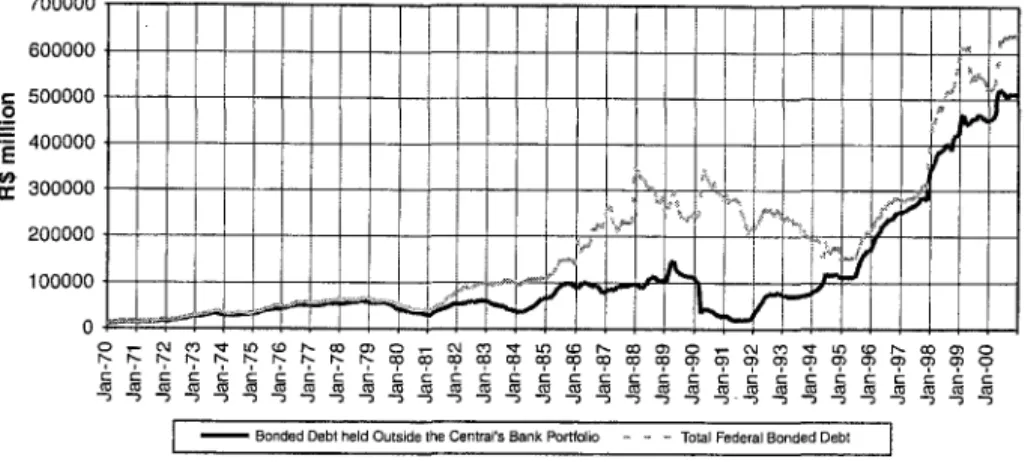
Figure I displays the evolution of the total federal government debt, separating the Central Bank holdings of government debt from the outstanding debt held by the private sector. During the high inflation years-from the early 1980s to the mid-1990s-there had been a widening of the fraction of the public debt
700000
600000
I:: 500000
,2
== 400000
E セ@ 300000
200000
100000
o
700000
600000
s: 500000 セ@ 400000
i
ftt
li: 300000 200000 100000
I
I i
I r
I セ@
i
i I セG@
I ,J " ...
I i I I
"
.
セセ@!
1\
iI
I ;,
I .t'1\r
.:\/
1\
l/"l
セj@
Jf
セ@I
",,""
"'"
Iiir
I,...
j
I i
A",_
セ@ セ@
"
./'r' ....J'i1
- Bonded Debt held Outside lhe Cenlral's Bank Partfalia セ@ - - Total Federal Bonded Oeb!
Figure L Federal bonds: 1970-2000.
Figure 2. Federal bonded debt structure: 1970-2000.
held by the Central Bank. Under high infiation, cash management activities tended to predominate in the banking sector and the Central Bank backing of such activities required the automatic provision of liquidity to banks' holdings of public debt. This situation stood in marked contrast to the stated objectives of the reforms. Nevertheless, the objective of institutional development of a market for government debt, which had been stated in the financiaI reforms of 1964-1965, had been attained.
The domestic public debt market in Brazil started with indexed bonds in the late 1960s. Only in August 1970, nominal bonds were placed (for the stated purpose of conducting monetary policy).2 Indexed bonds (ORTNs-Obrigações Reajustáveis do Tesouro Nacional) were seen by asset holders as a hedge against infiation-induced erosion of financiaI wealth despite the fact that, until 1974, monetary correction was arbitrarily defined each month by an act of the Ministry of Finance, without oflicial commitment to any particular price indexo
Without indexed bonds, the financiaI markets would not have developed as they did in the face of the
acce1erating annual infiation rates from 1973 to 1994. Figure 2 displays the remarkably mobile structure of
the Brazilian domestic public debt.
During the infancy of the public domestic debt market (1966-1971), the demand for public debt grew ahead of the government's financiaI needs. A large stock of public domestic debt was deemed convenient for regulating short-run liquidity of the banking system, by means of final sales and purchases of public
18 A.S. BEVILAQUA, M.G.P. GARCIA
r+
-500000 エMKMKMKKKKKKKMKMKMMKMMKMMKMMKMMMQMMMェMiMiMKMKMKMセセLJBB@
i 1-.
セ@ 400000 t-+-+-+-+-+-+-+-+-+-+-+ i l ⦅KMiKMIKェNNOMKセNNNNLNエNNM]KMKMKMKMKMKMKMMKMMMQ@
'E
300000 I--+-+--1--1--l-I-ᄋMMKMMKMMKMセャZMZMヲKMK@ ... MKMセMKMKMKMKMiMMMャMMQMMGMMi@w ⦅NiセQGMG@
IX: 200000 -I-..""l:r«-' --11-_ .... 1--1--1--+-1 -+-+-+-+-+---1---1-1--1--1--1--+--'----1
Nセ@
V
QPPPPPセセセセセセセセセセセKMセセセセセセセセセエ⦅エ⦅エ⦅エ⦅セ@
o
...
q>"S -,
...
LO LO LO l!)'"
'" '" '"
.... .... ....'"
'"
q> q> q>'"
q> q>'" '"
q> q>t;
c
c
t;c
'"
5. "S ti'"
5. "S'"
5. "SO -, <{ -, O -, <{ -, O -, <{ -,
- - Total Federal Bonded Oebt
.... <Xl
'" '"
.,!.c
"
'"
O -,
<Xl <Xl <Xl
q> q>
'"
t;
c:
"S<{ -, O
'" '"
'"
q>C
'"
5.-, <{
'"
q> "S -,'" o
'" o
8
セ@
Total Federal Bonded OebtlGOP
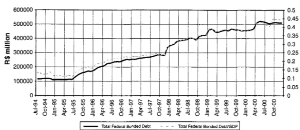
Figure 3. Federal bonded debt held Outside the CB's portfolio: the Real Plano
0.5
OA5 OA
0.35 0.3 0.25 0.2 0.15
0.1
0.05 O
debt in the open market. As in 'Say's law', however, the possibility of creating a large debt supply opened room for the creation, in the Central Bank, of a wide range of credit programs designed to fund agricultural projects and regional development, and has fostered the establishment of regional development banks at the state leveI. The excess demand for public bonds in the early years of the market led the Central Bank to
assume the role of a financing agent,3 an aberration that lasted for years. The development strategy of the
1970s was based in great measure on the public sector's ability to issue debt to fund development projects. By the late 1970s and early 1980s, it became clear that this growth engine had stalled. The decade witnessed high and unstable infiation, which led to a considerable increase in the volatility of the expected returns on government debt due both to a decline in the use of public savings and to frequent changes in monetary correction rules (i.e. partial disguised defaults). The 1980s are called the lost decade, due to the economic stagnation, the megainfiation, and the decline in public, as well as private, investment. As a consequence, the accumulation of public debt seemed to be approaching the end, and, by the turn of the decade, a default on domestic public debt was seen by many as an unavoidable outcome.
In fact, the new government whó took office in 1990 decreed the blocking of 80% of all financiai assets. The
terms of the decree were actually complied with, and the governmerit was able to unblock all the financiai assets beginning 17 months later, in 12 monthly instalments. During 1993-1994, capital infiows added to demand for high-yield public debt, creating a more stable environment that made the Real Plan possible.
2.2. Recent evolution: The Real Plan
In July 1994, a new currency, the Real, was introduced, as the last part of the de-indexation programo
Both the debt structure and size changed in important ways after the monetary reform, as the annual infiation rate fell from a four-digit figure to a one-digit figure. Until the Asian crisis (October, 1997), foreign capital kept fiowing in steadily, and the domestic public debt market experienced a period of gradual maturity lengthening due to decreasing yield volatilities. After the last quarter of 1997, a series of ups and downs has characterized the international finance scene for the emerging markets, also affecting the domestic public debt market. After a semester when more than US$45 billion of foreign reserves vanished, the Brazilian government decided to fioat the Real in January 1999, thereby inaugurating a new phase of the Plan. We analyse below the debt accumulation process since the introduction of the new currency, the Real, emphasizing debt size and structure (indexation and maturity).
2.2.1. Size. The extremely fast increase of the federal bonded debt during the Real Plan was one of the
macroeconomic indicators. Figure 3 displays the evolution of the federal bonded debt in constant R$ of
December 2000, and as percent of GDP. It is quite clear that, after remaining stable during the first year of
the new currency (July 1994 to June 1995), both measures of debt accumulation started trending upward.
WOOOOr---.18
wooqッエMMMMMMMMMMMMMMMMMMMMMMMMMMMMMMMMMMセセ[[セセセセセセQV@
14i
400000
イMMMMMMMMMMMMMMMMMMMMMMMMZZZ[ウ[[Zセセ@ 12l!
Si!
300000
t··· ...•......•... cc .... Jr. 10 1:6') B セ@
a:: 200000 エセセセMMMMMMMMNLNNZZsセ@ 6
1000001111
O セ@
セ@
-tiセo@
4
セセセセセセセP@ セセセPセセセ[NセセDQ@ 2
セセセセセセセセᄋo@
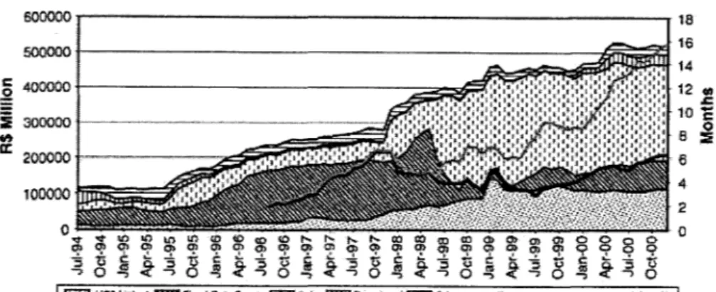
Figure 4. Federal bonded debt: composition and average maturity.
19
In nominal terms, the federal bonded debt increased by eight times in six years! Section 3 identifies the factors responsible for this enormous growth.
2.2.2. Composition. This section analyses the structure of the domestic debt, i.e. its composltlOn:
denomination of the debt (domestic currency versus foreign currency), indexation (to domestic price leveIs, to the exchange rate, to short-term interest rates, etc.), and maturity structure. We also explore new measures of risk exposure, as the V@R (Value-at-Risk).
2.2.2.1. Denomination and Indexation. AlI domestic federal bonded debt is redeemab1e only in R$. Only
the externaI debt is redeemable in foreign currency. Figure 4 displays the domestic federal debt composition
after the Real Plano It is c1ear that when the debt started trending upwards in mid-1995, it was the nominal
(non-indexed) part that was mainly responsible for the growth. Notwithstanding the increasing share of nominal in total debt, average maturity kept lengthening. Barcinski (1997) computed a measure of risk usualIy applied to financiaI institutions portfolios, the V@R for the nominal federal debt. The V@R measures the amount of market risk of a given portfolio, i.e. the maximum expected loss of that portfolio in
a given time span.4 He showed that, notwithstanding the increase in the nominal debt and its maturity
lengthening, the V@R of the nominal debt actualIy decreased for the first years of the Real Plan
(he analysed the period QYYセQYYVIN@ That refiected the fact that interest rate volatility was decreasing
substantialIy, except for the first semester of 1995, when it increased momentari1y as a consequence ofthe
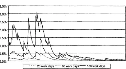
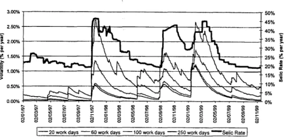
Mexican crisis. This falI in interest rate volatility is displayed in Figure 5.5
The share of nominal to total debt remained around SPセPE@ between July 1994 and November 1995,
when it started to grow, reaching 60% around mid-1996. That share was maintained until the Asian crisis, in September 1997, when it started to drop. Until the Russian crisis, in May 1998, the nominal debt share was stilI above 50%, despite the precipitous falI in average maturity. With the Russian crisis, the Treasury and the Central Bank started to issue only indexed debt (for reasons that will be analysed later), and the
nominal debt share felI to 3.5% in December 1998.6 After the nomination of the new Central Bank
governo r, in March 1999, this share has been increasing again.
The share of bonds indexed to the IGP-M (a wide1y used price index) decreased continuously during the whole period. According to Central Bank sources, that refiected a po1icy decision to stop issuing infiation-linked bonds, which were deemed infiationary.7 DolIar-infiation-linked bonds remained around 10% of the total debt between July 1994 and August 1995, falIing then slightly to around 7% of the total debt between September 1995 and February 1996. With the deterioration of the economic situation in Asia, it increased once again to reach 15% at the end of 1997. That share rose throughout 1998 to around 21 % at the year-end, showing that agents were (correct1y) hedging against the forecasted devaluation. The devaluation of January 13, 1999, and the continuous depreciation after the currency was fioated two days later,
increased the value of the dolIar-1inked debt vis-à-vis the other bonds. The share jumped to 30% after the
20 A.S. BEVILAQUA, M.G.P. GARCIA
SNUENMMMMMMMMMMMMMMMMMMMMMMMMMMMMMMMMMMMMMMMMMMMMMMMMMMMMMセ@
SNPEKMMMMMMMMMMMMMセMMMMMMMMMMMMMMMMMMMMMMMMMMMMMMMMMMMMMMセ@
RNUEKMMMMMMMMMセMMfKセMMMMMMMMMMMMMMMMMMMMMMMMMMMMMMMMMMMMMMセ@
RNPEKMセイMMMMMKイMMセセセMMMMMMMMMMMMMMMMMMMMMMMMMMMMMMMMMMMMセ@
QNUEゥMセQrセMMセセセセTMセMMMMMMMMMMMMMMMMMMMMMMMMMMMMMMMMMMセ@
QNPEセMMMMセセセセセセMMセMMMMMMMMMMMMMMMMMMMMMMMMMMMMMMMMMMセ@
• • •• 20 work days - 60 work days - - 100 work days
Figure 5. Daily Interest Rate Volatility: July-94 to Dec-96.
devaluation, and has fallen afterwards, as the demand for new issues of dollar-linked debt has diminished considerably and the currency appreciated after March 1999. With the new round of depreciation that started in May 1999, the demand for dollar-linked debt (or any hedge against depreciation) has been
increasing again, forcing the Central Bank to supply more of this kind of debt. 8
The share of bonds indexed to the short-run interest rate (or zero-duration bonds)9 was around 25% of the total debt between July 1994 and July 1995,35% between August 1995 and February 1996, falling to approximately 20% in November 1997. In December 1997, a large issue of this kind of bonds distorted all debt-statistics. Around R$ 50 billion of bonds were issued as part of a renegotiation deal with the Brazilian
state of São Paulo, \O making the share of zero-duration bonds jump to 35%. After that, as those bonds
were swapped with the Central Bank for shorter-maturity ones, their share fell gradually to 21 % in May 1998, when the beginning of the Russian crisis made the Central Bank and the Treasury change strategies regarding the issuance of nominal bonds. As mentioned before, the issuance of nominal bonds stopped, and only zero-duration bonds started being issued. That move made the share of the latter jump from 21 %
in May to 42% in June. By December 1998, the zero-duration bond share was almost 70%. It fell
in January due to the increase in value of the dollar-linked bonds, and it continued to fall later as the issuance of nominal bonds resumed after March 1999. As of December 2000, its share was hovering around 52.36%.
2.2.3. Maturity structure. Figure 4 shows the average maturity of the debt during the Real Plan. The
average maturity of the total debt has substantially increased in rei ative terms although it remains low in
absolute terms.lI It is nonetheless interesting that until the Asian crisis (September 1997), maturity kept
increasing despite the increasing share (and total value) ofthe nominal debt.12 As noted before, unti11996,
Barcinski (1997) showed that, the V@R of the nominal debt decreased despite the size increase and the maturity lengthening. In other words, investors in public debt were not incurring more price risk, despite the increase in the portfolio size and in the nominal debt maturity.
With the international financiai crises, this virtuous circ1e carne to an end. When Brazil began to suffer the contagion effect of the Asian crisis, in the form of a speculative attack during the week of October 27, 1997, the Central Bank quickly reacted by increasing the basic interest rate, the TBC, (see footnote 13) from 20.70 to 43.41 % (see Figure 5). After two weeks without public debt auctions, the rolling over continued with three-month-maturity bonds, at rates little below the TBC.
In that environment, the Treasury and the Central Bank probably did not want to issue long maturity debt. An interest rate of 43% per year (with the inflation rate well below 5% per year and an exchange-rate
SNPPEイMMMMMMMMMMMMMMMMMMMMMMMMMMMMMMMMMMMMMMMMMMMMMMMMMMMMMMMMMMMMMセ@
2.50% エMMMMMMMMMMMMMMMMMヲj|iNNLセイ⦅MMMMMMMMMMMM⦅LNLNNアヲ⦅MM⦅ヲ|⦅⦅i⦅iG⦅MMMMMMMMM⦅⦅i@
-;;:-lO
!:. 2.00% エMMMMMMMMMMMMMMiiMM|ZMMM]GエMMMMMMMMMiiMMMMGLMMLiMNNャljセャ⦅⦅MMMMMMMM⦅]Q@
セ@
8. セ@
1.50%
エMpセ[MZMMMMMMMMMMKMMセMMMKMMMMMMMMiセMMMMMMャiaイM⦅K⦅ャ⦅MMMMMMM⦅K@セ@
=
セ@ QNPPEKMMMMMMMMMセセセセセセMMセセMMMMセセセセセセセセセセセイ⦅セZZセZZゥ@
セ@
....
.... ........
co co co co co co'"
8l O>'"
'"
'"
I!! Dl I!! $ I!! I!! I!!セ@ I!! $ I!! I!! セ@ セ@ $
OI) r::: CJ)
セ@
'" '"
mセ@
M OI)セ@ セ@ o (;J セ@ o (;J !2 N o (;J o (;J セ@ セ@ セ@ セ@ !2 N (;J
o o o o o o o o o o o o o o o o
1-20 work days -SO work days -100 work days -250 work days -Selic Rate
I
Figure 6. Levei and Volatility of Interest Rate: The Crises Period.50% 45% 40% -;;:-35%
..
!:.30% ; 1:1.
25% セ@
S
20% 11(
..
15% .!! G
UI
10% 5% 0%
devaluation of 7.5% per year) is clearly unsustainable in the long run, being sustainable only briefiy to counteract a speculative attack. Therefore, had the Treasury and the Central Bank decided to place one or two year bonds at such a high rate, they could conceivably have sparked a panic, because of the informational content of such a move. Placing debt at 43% for short periods might be desirable, but paying such high rates for long periods puts the government budget on a c1early unsustainable path. That could then trigger expectations of a government default. In other words, in such a situation, there may be no equilibrium with such a high interest rate and long maturityY The only equilibrium may be the one with very short maturity bonds. An alterna tive explanation is that the maturity premium demanded by the market for longer maturity bonds was beyond the maximum premium implied by the auction managers'
reservation prices.14 That rollover strategy had the effect of decreasing the maturity of the stock of debt.
Figure 6 shows that interest rate volatilities increased tenfold during this turbulent period. As a
consequence, so did the V@R measures. '
Until the end of 1997, only three-month maturity bonds were placed, alI with negative maturity
premia. During the first five months of 1998, the Treasury and the Central Bank were able to place nominal
debt with increasing maturity. However, when the Russian crisis first hit in May 1998, even short-term bonds (three or six months) became extremely cost1y for the issuers, as yields rose substantially. As a consequence, the market for three-month, six-month and one-year bonds vanished, and the only nominal
bonds placed in the auctions after mid-May were one-month BBCs.15 In June and July, even that became
too expensive, and the Central Bank resorted to its last resource, the zero-duration bond.
This decision had an immediate impact on the amounts that were rolled over in each auction. When the debt maturity decreases, the debt must be rolled over more often. That is exact1y what was happening until May 1998. The amounts of monthly redeemed and issued debt tripled! This, of course, created a new source of risk-the rollover risk-i.e. that of not being able to rolI over the debt in the event of a crisis, with possible impacts in the exchange-rate anchor that was in place at the time. After May, due to the strategy of placing only indexed bonds (most1y zero-duration and dolIar-linked), average maturity resumed its upward trend, and the rollover risk decreased. However, this happened at a cost: if interest rates had to be lifted in the future, the fiscal budget would be badly hit. The same was valid regarding a devaluation. With the benefit of hindsight, we know now that both strategies caused massive losses to the fiscal budget, Even with zero-duration debt, average maturity felI again in the last quarter of 1998, due to the contagion effect of the Russian default. After the devaluation, maturity has been increasing (see Figure 4). However, if the government were now to decide to quickly change the current debt structure in favour of nominal debt, either a fall in maturity or a substantial cost increase in debt service would be likely, as we will discuss in Section 5.
22
A.S. BEVILAQUA, M.G.P. GARCIAJ.EVOLUTIQN OF THE GROSS DOMESTIC BONDED DEBT DURING THE REAL PLAN:
, A DECOMPOSITION EXERCISE
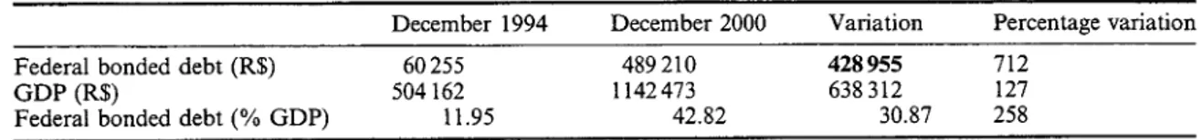
'\)lU1ng the first six years of President Fernando Henrique Cardoso's administration, the federal bonded debt increased to more than eight times its original value: from R$ 60 billion to R$ 489 bilIion (see footnote 12). This spectacular debt growth raises many doubts about the sustainability of economic policy, especialIy if one considers the effects of the exchange-rate devaluation in January 1999, which increased even further the service costs of federal bonded debt, due to the existence of dolIar-linked indexation clauses on part of the debt.
This section decomposes the federal bonded debt growth, searching for the macroeconomic causes ofthe considerable growth that occurred in the 1995-2000 period. We attempt to quantify the contraction and expansion sources of the federal bonded debt.
Consider the federal government and Central Bank aggregate balance sheets on 31 December 1994 and 31 December 2000, respectively. One of the accounts on the liability side is the federal bonded debt. The value we are interested in explaining is the difference between this account's balances on these two dates. Due to accounting identities, this value is the sum (with opposite sign) of the differences during the period of alI the other accounts' balances. Consequently, by aggregating these other accounts' balances in a way amenable to our macroeconomic analysis, we measure the factors responsible for the growth of the federal bonded debt in this four-year period. The idea of this decomposition exerci se can be better understood with the accounting framework provided in Table 1. The table starts from the government budget constraint, and develops an accounting identity (Equation (6» that is suitable for our purpose of identifying the sources of the growth of the federal bonded debt.
Thus, we search for an explanation for the R$428955 variation, as shown in Table 2, of the federal bonded debt (federal government + Central Bank).
InitialIy, we wilI aggregate the other accounts in the federal government and Central Bank aggregate balance sheet into three groups, each one of them standing for one of the folIowing reasons to issue federal bonded debt,16 as laid out in Table 1.
(1) To finance the federal government's (+Central Bank's) deficit (2) To accumulate foreign and domestic assets; and
(3) To repay other previous debts (non-bonded debt).
Table 1. Debt uses: a decomposition (1) Net debt = Liabilities-assets
(2) A(Net debt) = A(Liabilities)-A(assets)
(3) A(Net debt) = Primary deficit + interest payments + adjustments
(4) A(Liabilities) = A(domestic bonds) + A(other domestic debt) + A(foreign debt)
(5) A(Assets) = A(domestic assets) + A(foreign assets) (3), (4), (5)
'*
(2), and solving for A(Domestic bonds) Source of funds = Uses of funds(6) A(Domestic bonds) = Primary deficit + interest payments + Adjustments + A(domestic assets) + A(foreign assets)-A(other domestic debt)-A(foreign debt)
Table 2. Federal bonded debt growth: 1995-2000
Federal bonded debt (R$) GDP (R$)
Federal bonded debt (% GDP)
December 1994 60255 504162
11.95
Copyright © 2002 John Wiley & Sons, Ltd.
December 2000 489210 1142473
42.82
Variation
428955
638312 30.87
Percentage variation 712
127 258
Table 3. Federal bonded debt uses: 1995-2000
December 1994 December 2000 Variation
nセャ@
","t
(increase = deficit)セGQゥゥ・エ@ accumulation
Other debts' repayments (-)
Total
65836 106559 112140
In percent of GDP, the data above are:
352967 376881 240639
287131 270323 128499
428955
Table 4. Federal bonded debt uses in percent of GDP: 1995-2000
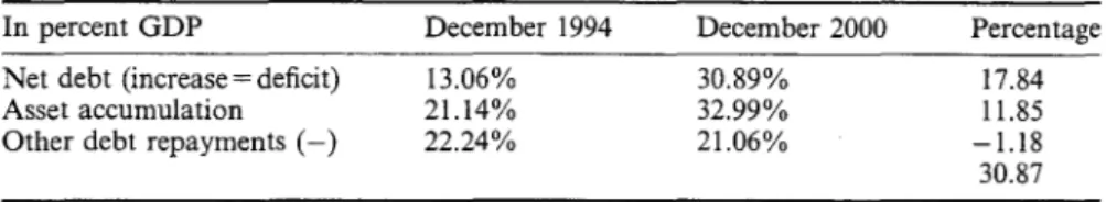
In percent GDP
Net debt (increase = deficit) Asset accumulation Other debt repayments (-)
December 1994
13.06% 21.14% 22.24%
December 2000
30.89% 32.99% 21.06%
Percentage variation 436.1
253.7 114.6
Percentage 17.84 11.85 -1.18 30.87
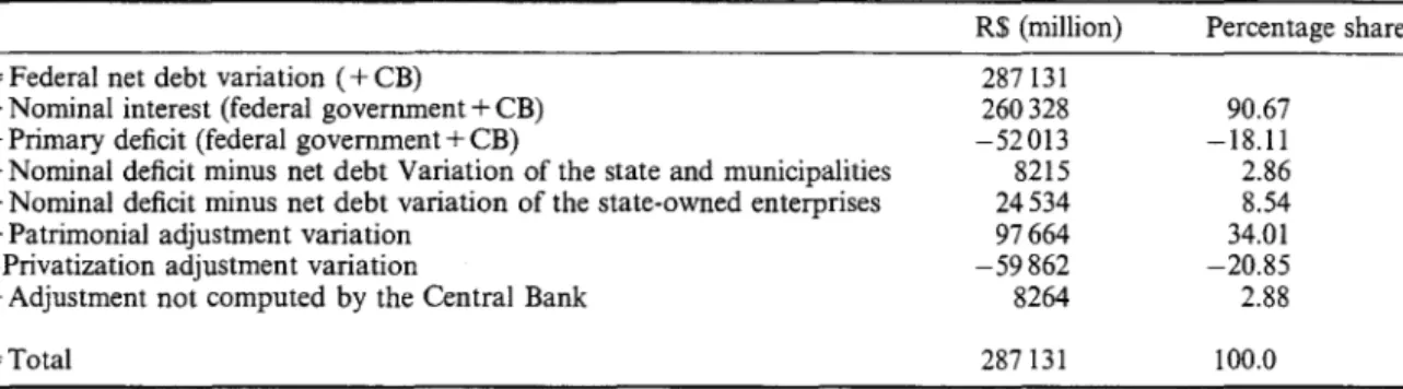
Item 1 represents the difference in the two net worth figures (a fiscal deficit is a loss, and a fiscal surplus is a profit); item 2, the asset accumulation during the period; and the item 3, the decrease in the aggregate of ali other liability accounts. Thus, considering the federal bonded debt as the 'sources', and the other accounts as the 'uses' we can observe these uses in Tables 3 and 4, expressed in R$ and percentage of GDP, respectively.17
Table 3 shows the federal bonded debt variation. The greatest share (66.94%) of the increases in federal
bonded debt was due to the federal deficit (which would be equal to the net debt variation, if it were not for
accounting details discussed above). The accumulation of assets was responsible for a little bit less, 63.02% of the federal bonded debt growth. The increase in other debts was responsible for the (negative) residual factor (29.96%), which means that ifthe other debts had not grown by R$128499, the federal bonded debt would have increased even more. Measured as a share of GDP, the federal deficit was responsible for 57.78% of federal bonded debt growth of 30.87% of GDP (Table 4). The accumulation of assets was responsible for 38.40% of the federal bonded debt growth, while the other debts actually decreased as a
percent of GDP, being responsible for the remaining 3.82% of the federal bonded debt growth.18
We now turn to the decomposition of each of these three factors: the federal deficit, the assets accumulation, and the repayment of other debts.
3.1. Financing of lhe Federal Government (+ Central Bank) Dejicit
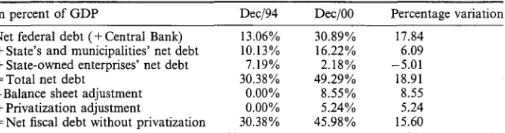
In order to make the net debt variation of the period (R$ 287131 or 17.84% of the GDP) compatible with the nominal deficits registered during the same period, it is necessary to make three adjustments. The first is to add the states', municipalities' and state-owned enterprises' net debt variation.
The second adjustment recognizes the privatization revenues. Since privatization revenues occur only once; they are not inc1uded in the public deficit computation. Nevertheless, they are public revenues which,
ceteris paribus, would lower the net debt (the state-owned enterprises that were sold were not previously
included in the public sector assets). Keeping the hypothesis that everything else stayed constant, and assuming that all the privatization revenues were used for public debt redemption, the gross debt would diminish by the exact amount of these privatization revenues. Therefore, we have to add these revenues to the variation of the total net debt in order to obtain the debt variation concept that best conforms to the
public deficit statistics.19
24 A.S. BEVILAQUA, M.G.P. GARCIA
The third adjustment is related to the 'Balance Sheet Adjustment.2o The ide a ofthis adjustment is that the
macroeconomic impacts of the 'skeletons' (old debts that were eventually repaid) occurred in the past. For example, the public debt issue for Banco do Brasil's recapitalization-whose accumulated losses were threatening its solvency-recognized losses derived from bad credit expansions in the past. Indeed, the
debt issue was not related to deficits during the recapitalization period, but to old deficits, that had never
been recognized until then. Thus, it is necessary to subtract the Balance Sheet adjustment's variation from the total net debt to obtain the debt variation concept comparable to the public deficit, namely, the 'Net Fiscal Debt without Privatization'.
Therefore, the following accounting identity should hold: for the fiscal statistics published by the Brazilian Central Bank.
Increase in net fiscal debt without privatization = nominal deficit
Making the adjustments, we obtain
Table 5. Making compatible the net federal debt statistics and the nominal debt statistics in R$: 1995-2000
In R$ (million)
Net federal debt (+ Central Bank)
+ State's and municipalities' net debt
+ State-owned enterprises' net debt
= Total net debt
- Balance sheet adjustment
+ Privatization adjustment
= Net fiscal debt without privatization
Decj94 65836 51091 36236 153163 O O 153163 DecjOO 325967 185323 24873 563163 97664 59862 525360 Variation 287131 134232 -11363 410000 97664 59862 372197 Percentage variation 436.13 262.73 -31.36 267.69 243.01
Table 6. Making compatible the net federal debt statistics and the nominal debt statistics in
percent of GDP: 1995-2000
In percent of GDP
Net federal debt (+ Central Bank)
+ State's and municipalities' net debt
+ State-owned enterprises' net debt
=Total net debt
- Balance sheet adjustment
+ Privatization adjustment
= Net fiscal debt without privatization
Decj94 13.06% 10.13% 7.19% 30.38% 0.00% 0.00% 30.38% DecjOO 30.89% 16.22% 2.18% 49.29% 8.55% 5.24% 45.98% Percentage variation 17.84 6.09 -5.01 18.91 8.55 5.24 15.60
Table 7 shows the evolution and the composition ofthe public deficit during the 1995-2000. The net federal debt variation is slightly higher than the nominal deficits accumulated in the same period
(372 199-363933 = 8264). This difference occurred during 1995, when the Balance Sheet adjustments'
methodology was not yet implemented. Therefore, an extra item will be inc1uded, 'Adjustment not computed by the CB', amounting to R$ 8264 million.
After all these adjustments, the equation which links the federal debt variation (+ CB with the federal nominal deficit is expressed in Table 8. It shows that largest share of item I, which can be identified with the
financing of the federal public debt (+ CB), was due to interest payments (90.67%). Item I's second biggest
expansion source was the Balance Sheet adjustment. Note that this expansion effect from the Balance Sheet adjustment (34.01 %) was substantially weakened by the privatization's contractionary effect (-20.85%). As we have already discussed, none of these items constitutes exactly the public deficit. According to the definition of the federal deficit, neither of the other items-related to states and municipalities (2.86% of
Table 7. Public sector borrowing requirements: 1995-2000
In R$ (million) 1995 1996 1997 1998 1999 2000 Accumulated
Nominal 47027 45741 53232 72490 96158 49285 363933
Federal govemment and CB 15392 19946 22912 49361 66209 34496 208315 States and municipalities 23067 21076 26377 18416 30589 22291 142447
State-owned enterprises 8568 4720 3943 4713 -640 -8132 13171
Nominal Interest 48750 45001 44923 72596 127245 87442 425958
Federal govemment and CB 18728 22853 20537 54402 88881 54926 260328 States and municipalities 21915 16840 19941 16686 32694 28947 137023
State-owned enterprises 8108 5308 4444 1508 5670 3569 28606
Primary -1723 740 8310 -106 -31087 -38157 -62024
Federal govemment and CB -3336 -2908 2375 -5042 22672 -20431 -52013 States and municipaJities 1152 4236 6436 1731 -2105 -6026 -5423
State-owned enterprises 461 -589 -501 3204 -6310 -11700 -15435
Table 8. Making the federal net debt statistics and the federal nominal deficit compatible: 1995-2000
= Federal net debt variation (+ CB)
+ Nominal interest (federal governrnent + CB)
+ Primary deficit (federal governrnent + CB)
+ Nominal deficit minus net debt Variation of the state and municipalities
+ Nominal deficit minus net debt variation of the state-owned enterprises
+ Patrimonial adjustment variation -Privatization adjustment variation
+ Adjustment not computed by the Central Bank = Total
R$ (million) 287131 260328 -52013 8215 24534 97664 -59862 8264 287131
Percentage share
90.67 -18.11 2.86 8.54 34.01 -20.85 2.88 100.0
item I's growth) and the state-owned enterprises (8.54%)-should be inc1uded, since this item (I) refers only to the federalleve1. 21 The federal government and Central Bank's primary deficit had a contractionist impact during this period (-18.11 %).
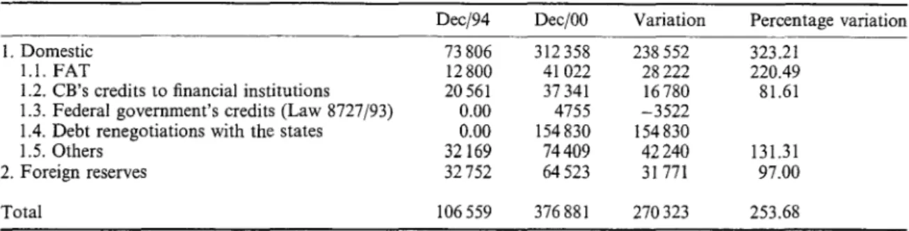
3.2. Accumulation 01 assets
Table 9 decomposes the accumulation of assets during this period. Note that domestic assets growth (323.21 %) was substantially greater than the foreign assets' growth (97%). The growth rates are unequal among the domestic assets also. The states' debts renegotiation, which appears in items 1.3 and 1.4, is responsible for slight1y more than half of this increase (63.43%).22 The Central Bank's credits to financiai institutions, which inc1ude the Proer (the private banks' bailout programme), played a minor role: 7.03%.
3.3. Repayment olother kinds 01 federal public debt
26 A.S. BEVILAQUA, M.G.P. GARCIA Table 9. Assets accumulation in R$: 1995-2000
Dec/94 Dec/OO Variation Percentage variation
1. Domestic 73806 312358 238552 323.21
1.1. FAT 12800 41022 28222 220.49
1.2. CB's credits to financiai institutions 20561 37341 16780 81.61
1.3. Federal govemment's credits (Law 8727/93) 0.00 4755 -3522
1.4. Debt renegotiations with the states 0.00 154830 154830
1.5. Others 32169 74409 42240 131.31
2. Foreign reserves 32752 64523 31771 97.00
Total 106559 376881 270323 253.68
Table 10. Other debt variations: 1995-2000
Dec/94 Dec/OO Variation Percentage variation
1. Other domestic debt 46947 90721 43774 93.24 1.1. Monetary base 17685 47679 29994 169.60
1.2.0thers 29262 42042 13780 47.09
2. Foreign debt 65193 149918 84725 129.96
Total 112140 240639 128499 114.59
growth was smaller than the foreign one (93.24% versus 123.96%). Among the domestic net debt components, the greatest share is due to the Monetary Base, responsible for 23.34% of the total net debt variation.
Table II summarizes the discussion about the factors of expansion and contraction of the federal public debt (in nominal terms). One must keep in mind that, since we are working with nominal values
over a period of four years, the values presented in this table can be misleading.23 It is observed that the most important facto r for debt growth was interest payments (60.69%), followed by the accumulation of the state's debt (36.09%). If we add these interest payments to the accumulation of domestic assets, the quality of which is uncertain, we can 'explain' more than 99% of the debt growth in this period.24 Therefore, it is quite reasonable to identify public debt growth with the deterioration of the fiscal
position.
Table 12 summarizes the discussion about the factors of expansion and contraction of the federal public debt (in real terms). The analysis in real terms generates a few discrepancies from the previous analysis, and,
of course, is the most relevant to the current economic situation. The interest rate share increased even more in real terms: interest payments (27.07% of GDP) alone exceeded the full variation of the federal net debt (17.84% of GDP). Foreign Reserves actually fell as a % of GDP (0.85%), thereby making the whole Asset Accumulation much less attractive as an indicator of solvency.
A word of caution is necessary. One should not infer from the previous analysis that the bulk of the explosive growth in domestic bonded debt was due exc1usively to the policy of extremely high interest rates, and that had the interest rates been lower, the bonded debt would not have exploded. Interest rates were high not only because of the Central Bank policy decisions, but mainly because the fiscal stance became increasingly lax as the first successes of the Real Plan appeared on the inflation front. 25 Bevilaqua and Werneck (1998) show that the primary balance of the consolidated
Table 11. Federal debt uses in R$: 1995-2000 (R$ Millions)
Dec-94 Dec-OO
Federal net debt (+ CB) 65836 352967
Nominal interests (Federal govemment + CB)
Primary deficit (Federal govemment + CB)
Nominal deficit minus net debt and variation of the states and municipalities
Nominal deficit minus net debt variation of the state-owned enterprises
Balance sheet adjustment variation Privatization adjustment variation (-) Adjustment not computed by the Central Bank
Assets 106559 376881
1. Domestic 73806 312358
1.1. FAT 12800 41022
1.2. CB's credits to the financiai institutions 20561 37341
1.3. Federal govemment's credits (Law 8727/93) 8276 4755
1.4. Debt renegotiations with the states O 54830
1.5. Others 32169 74409
2. Foreign reserves 32752 64523
Other debts (-) 11240 240639
1. Domestic 46947 90721
1.1. Monetary base 17685 43042
1.2. Others 29262 149918
2. Foreign 65193
Total
Table 12. Federal debt uses in percent of GDP: 1995-2000
Federal net debt ( + CB)
Nominal interests (federal govemment + CB)
Primary deficit (federal govemment + CB)
Nominal deficit minus net debt variation of the states and municipalities Nominal deficit minus net debt variation of the state-owned enterprises Balance sheet adjustment variation
Privatization adjustment variation (-) Adjustment not computed by the Central Bank
Assets
I. Domestic
1.1. FAT
1.2. CB's credits to the financiaI institutions 1.3. Federal Govemment's credits (Law 8727/93) 1.4. Debt Renegotiations with the states 1.5. Others
2. Foreign Reserves
Other debts (-)
I. Domestic
1.1. Monetary Base 1.2.0thers 2. Foreign
Copyright © 2002 John Wiley & Sons, Ltd.
Dec-94 13.06% 21.14 14.64 2.54 4.08 1.64 0.00 6.38 6.50 22.24 9.31 3.51 5.80 12.93 Variation 287131 260328 -52013 8215 24534 97664 59862 8264 270323 238522 28222 16780 -3522 154830 42240 31771 -128499 -43774 -29994 -13 780 -84725 428955 Dec-OO 30.89% 32.99 27.34 3.59 3.27 0.42 13.55 6.51 5.65 21.06 7.94 4.17 3.77 13.12 Percentage share 93.24 60.69 -12.13 1.92 5.72 22.77 -13.96 1.93 63.02 55.61 6.58 3.91 -0.82 36.09 9.85 7.41 -29.96 -10.20 -6.99 -3.21 -19.75 100.00 Variation 17.84% 27.07 -5.09 0.91 2.90 9.91 -6.01 0.98 11.85 12.70 1.05 -0.81 -1.23 13.55 0.13 -0.85 1.18 1.37 -0.67 2.04 0.19
28 A.S. BEVILAQUA, M.G.P. GARCIA
public sector deteriorated substantially during 1994-1998, while it improved remarkably in the following years.
4. CHALLENGES AHEAD: DEBT EVOLUTION IN THE POST-DEVALUATION PERIOD
In this section we perform simulations of the public net debt path to 2012. The starting point for the derivation of the model used for the debt-dynamics simulations is the standard budget constraint of the consolidated public sector, which in the case of Brazil includes the central government, states and municipalities and public enterprises:
Mt - Mt-I Bt - Bt-I Et(B; - B;_I)
----+
+--'---'----'-"":"!'"
Pt Pt Pt
Dt . Bt- I .*Et * At H t
=:-+lt--+lt-Bt
1--+-Pt Pt Pt - Pt Pt
(1)
where M is the monetary base, B is the net domestic debt, B* is the foreign debt net of international
reserves, E is the nominal exchange rate in R$ per US$, D is the primary deficit, i is the domestic interest
rate, r is the foreign interest rate, A denotes privatization revenues and H represents hidden and contingent
liabilities.
It is useful to rewrite Equation (1) in terms of fiows and stocks per unit of domestic product:
Mt - Mt-I
+
Bt - Bt-I+
Et(B; - B;_I)PtYt PtYt PtYt
Dt . Bt-I .* Et * At Ht
=: PtYt
+
lt PtYt+
lt pty/t- I - PtYt+
PtYt(2)
or
(3)
where (l, d, a and h are, respectively, seignorage, primary deficit, privatization revenues and hidden and
contingent liabilities in terms of GDP.
Equation (3) can be further rearranged as
b I
+
b* I -- Bt- I (1 /+
it)+
Et-I b* t-I EI (1 /+
i;) - (lI+
dt - at+
hl (4)PI- I YI- I PtYI Pt- I Yt- I PI- I Yt-I EI_I PtYt Pt-I YI-I
or
(5)
where b and b* are, respectively, net domestic debt and net foreign debt in terms of GDP, n is the infiation
rate, n is the real GDP rate of growth and eis the nominal exchange rate of depreciation.
Equation (5) may be used to simulate the path of the net domestic debt in Brazil over the medium term taking into account specific assumptions about the primary deficit, infiation rate, rate of growth of real GDP, nominal exchange rate devaluation, domestic and foreign interest rates, and seignorage revenues. In addition, since the government intends to continue its privatization programme, one needs to make assumptions about how that programme will be implemented. Finally, it is necessary to take into account the fact that the government has hidden and contingent liabilities which will be recognized in coming
years.26
To simulate the public debt path in the coming years, we will make use of Monte Carlo simulation.
Therefore, in each scenario, instead of assuming a deterministic path for a given exogenous variable,
we will make assumptions about their stochastic processes. For the years 2001 and 2002, we will make use
Table 13. Detenninistic variablese paths Detenninistic variables
Nominal depreciation (R$fUS$) Domestic inflation rate (IPeA) Privatization
Hidden liabilities
2001 25.29%"
6.53%" 1.00% 2.50%
'Market expectation (FOCUS-BCB-23jlljOI).
2002 6.12%" 4.50%" 1.00% 1.50%
2003 1.0% 3.25% 0.50% 1.00%
Table 14. Stochastic variables paths
Random variables Primary surplus Real GDP growth
Nom. dom. interest rate 2003
Nom. dom. interest rate 2012
Distribution Truncated lognormal Truncated nonnal Triangular Triangular
Min 0.00% 2.25% 6.00% 6.00%
2004 1.3% 3.25% 0.50% 1.00%
Mean 3.00% 4.00% 9.67% 8.01%
2005-2012 1.3% 3.25% 0.50% 0.50%
Max 4.00% 5.75% 13.00% 10.00%
of market expectations information published by the Brazilian Central Bank (www.bcb.gov.br) on Novem ber 23, 2001.
We will work with two scenarios. The first scenario-the status quo scenario-basically assumes that the
current IMF agreement until the end of 2002 will be strictly followed, and that the fiscal surpluses will be retained in the years after 2002. That amounts to a primary surplus of 3.4% of GDP in 2001, and 3.5% in 2002. For the period 2003-2012, the primary surpluses are independent1y drawn from a truncated lognormal distribution with mean 3%. Infiation is assumed equal to the market expectation values, name1y 7.4 and 5.59% for 2001 and 2002, respectively. After that, we assume that the infiation target for 2003, 3.25%, wiU be repeated until the end of the simulation period. Nominal depreciation is set for 2001-2002 according to market expectations, and, after that is kept constant at 1.25%. The real interest rate is drawn from a triangular distribution whose mean declines monotonically during the simulation period (see Table 2). The nominal interest rate is obtained interacting the infiation with the real interest rate. Real GDP is supposed to grow by 1.7% and 2.0% for 2001 and 2002, according to market expectations. After that, the fall in real interest rates allows for greater real GDP growth. Those rates are drawn from a truncated normal distribution with mean equal to 4%. For 2001, the interest rate on the externaI debt is assumed to
be equal to 11 %, and, after that, is determined by uncovered interest arbitrage, assuming that expected
depreciation equals actual depreciation. Seignorage is determined through the assumption of a constant monetary base for 2001 and 2002, and, after that, a constant monetary base as a share of GDP. Privatization revenues were assumed equal to 1% of GDP for both 2001 and 2002, and 0.5% after that. Hidden liabilities were assumed equal to 2.5% and 1.5% ofGDP for 2001 and 2002, respectively, and 0.5% after that. Tables 13 and 14 summarize the assumptions just described. Table 13 explains the deterministic variables evolution, while Table 14 displays the assumptions used to determine the stochastic variables paths.
Given these hypotheses, the simulation of one thousand paths provided the evolution displayed in
Figure 7, where the debtjGDP ratio has a hump-shape, declining after 2004. The histogram for the Debtj
GDP ratio in the final year, shown in Figure 8, has a mean of 49.5%. The simulation 90% confidence interval is (42%, 58%). Therefore, a 5% V@R would be 58%, meaning that according to our simulations
there would be only a 5% probability of the DebtjGDP ratio being greater than 58% in 2012.
The second scenario is constructed so that we may appreciate the effect of the DebtjGDP path of a more
lax fiscal stance. We achieve that by decreasing the average fiscal surplus in 1% of GDP every year after 2002, i.e. from 3 to 2% of GDP. The results are displayed in Figures 9 and 10.
30 A.S. BEVILAQUA, M.G.P. GARCIA
VUEイMMMMMMMMMMMMMMMMMMMMMMMMMMMMMMMMMMMMMMMMMMMMMMMMMMMMMMMMMMMセ@
60%
55%
50%
45%
TPEセMMセMMMMセMMセMMMKMMMMセMMセMMセMMMMKMMMセMMセMMMMセMMMKMMセ@
1999 2000 2001 2002 2003 2004 2005 2006 2007 2008 2009 2010 2011 2012
Figure 7. Debt-GDP ratio.
8.0 ,--- ---,---...,---...,
7.0 6.0
5.0 4.0
3.0 2.0
1.0
0.0 +-__ NNN」N]ZZZeNNMNQliQZNNNーNセセ@
0.30 0.41
x <=.42 5%
0.53
x <= .58 95%
Figure 8. Debt-GDP ratio.
0.64 0.75
With this slight change in the fiscal stance, the DebtjGDP path loses its hump shape, and exhibits
a monotonically increasing trend. The new 90% confidence interval becomes (53%, 70%). With such results, it is likely that fears of a default would increase interest rates, making the end result even those displayed here.
Therefore, two conc1usions are derived from the simulation results. First, unlike much of the opinions
expressed by international banks and a few eminent academics since 1997, the Brazilian DebtjGDP path is
not necessarily in an unsustainable path, provided that the current strict fiscal stance remains. Second,
unlike many suggestions that c1aim that the increase in the DebtjGDP ratio was caused only by the high
interest rates, and by consequence that a more lax fiscal stance would be possible in the future provided that
interest rates were reduced, we have shown that a slight fall in the primary fiscal surplus may put the Debtj
GDP ratio in an unsustainable path.
5. POLlCY DISCUSSION
As the simulation results from the previous section indicate, even under very favourable macroeconomic conditions the evolution of the net debt to GDP ratio will remain a policy concern in coming years. U nder these circumstances, what role should be played by public debt management in the near future?
75%.---,
70%
65%
60%
55%
50% ... _ - /
TUEKMMMセMMセMMMMKMMMセMMセセMMセMM⦅KMMMMセMMセMM⦅KMMMMセMMセMMセ@
1999 2000 2001 2002 2003 2004 2005 2006 2007 2008 2009 2010 2011 2012
I [ZエZZコZセキエZ[ゥ@ + 1 se, ·1 SO _ +95% Perc, -5% fere - - - Mean
Figure 9. Debt-GDP ratio.
8.0 , - - - -MMMMMMM[Z]]]]セ@
- - - ,
7.0 6.0 5.0
4.0
3.0
2.0
1.0
0.0 1-____ ]BBNャ[ZZZZZ[[[ZZiャ、ゥ[[Bオセ@
0.40 0.51
x <= .53 5%
0.63
x <=.7
95%
Figure 10. Distribution of net debt in 2012.
0.74 0.85
We see public debt management as constrained by a fundamental policy consideration in the short run. Although perceptions about the likelihood of a debt rollover crisis in Brazil has improved considerably since the January 1999 devaluation, the large stock of short-term debt remains an important source of anxiety, especially on the part offoreign investors. Even ifthere are reasons to believe that such a concern is somewhat misplaced,27 a practical implication of this fact is that the risk premium on Brazilian securities remains higher than what it would likely be if the same public sector borrowing requirements were financed with longer maturity debt. A central priority of debt management in the short and medium run, therefore, should be to intensify efforts to lengthen the average maturity of the public debt. Furthermore, given the need to reduce the interest burden of the debt and increase the sustainability of the current fiscal stance, such maturity lengthening should naturally be imp1emented at the lowest possible cost.
What kind of debt instruments will be more appropriate under these conditions? It is expected that under
the current IMF-supported programme the share of externai and foreign-exchange-indexed debt in the total public debt will be reduced gradual1y. Therefore, the process of debt maturity lengthening must be conducted through the issuance of domestic debt, either nominal or indexed.
32 A.S. BEVILAQUA, M.G.P. GARCIA
' ..
/.
What
sィojャャセNセセ@
ᅳセM・@
rei ative shares of these instruments in debt placements? For the sake of clarity of the・クーッウ■エゥッセ@ .•
!we
partition the question of how much of each kind of debt should be issued in two layers. First,we ・セ|ャャゥョ・@ how much nominal against indexed debt should be issued. Second, among the severa I kinds of
,.,,"tlxed
debt, how much of each kind should be issued (zero-duration and inflation-linked). Although the determination of the debt structure is a multiple-choice allocation problem, the two-Iayered scheme is adequate for the Brazilian case, as we now explain.To lengthen the average maturity of the debt requires the issuance of indexed debt, since long nominal debt (above two or three years) can only be issued at an abnormally high-risk premium. Therefore, the basic policy recommendation concerning the public debt structure for the Brazilian economy in the coming months is to issue nominal debt with the highest possible maturity without creating an extremely upward-sloping yield curve at the end. For the time nodes previously 'conquered', issue the highest possible amount that do not create 'price-pressure' effects. For the bulk of the rollover and for the new additions to the debt stock, indexed debt should be issued, to lengthen the maturity structure as much as possible.
In terms of placement procedures, the authorities should announce the auctions as far in advance as possible28 and avoid placing unexpected amounts of short-term securities in order to profit from the low maturity premia of the shorter maturities. Placing short-term debt because it is cheaper in an environment of lack of confidence jeopardizes the situation of the previous long-debt holders, because the short-debt
holders have a liquidation option over those, and harms the debt market in the long run. It is akin to the
issue of debt seniority: the short-term debt holders hold debt that is senior vis-à-vis the long-term
debt holders, since the former will mature before the latter. Information regarding the process of debt lengthening must be well conveyed to the market, so that debt holders know in advance that they will be purchasing liquid instruments, and that the government will not 'cheat' on them by placing shorter instruments in the future.
An important question remains on how much of each kind of indexed debt Czero-duration, intlation-linked, exchange-rate-linked, or another form as discussed below) should be issued. The exchange-rate-linked debt share, as already mentioned, must conform to the guidelines of the current IMF-supported programme. Given the current intlation-targeting framework the use of zero-duration debt poses a version of the well-known time consistency problem. The over reliance on zero-duration debt, as in the current situation with 50% of total debt in this form, may reduce monetary policy credibility and commitment, because policy makers may become more exposed to choices and trade-offs between tight money policies to contain inflation and the budgetary impact of higher short-term rates. Therefore, it is advisable to reduce the share of this kind of indexed debt in the total public sector debt.
Therefore, the remaining instrument to be used in the process of maturity lengthening is intlation-linked debt. The main objection to this kind of debt indexation is that it may have intlationary effects.
Nevertheless, as Price (1997) emphasizes C ... ) the academic literature suggests no necessary connection
between indexed bonds (or indexation in general) and inflation. The emergence of inflation depends on other circumstances and policies that are independent of indexation. Recent government issuers of indexed bonds in fact point to credibility enhancements that may result from issuing indexed bonds, by neutralizing the inflation
tax (p. 53). Price's advice is that ( .. .) in newly developing or transition markets, they [indexed bonds] could
be envisaged as part of a concomitant package of fiscal and monetary reforms to foster longer-term capital
formation, along with strong commitments to price stability (p. 55).
The current share of intlation-linked debt is negligible. This was a result of a policy decision after the Real Plan, when debt managers-convinced that intlation-linked debt was intlationary by conveying to the market a lack of anti-intlationary commitment of the government-decided to phase it out. Our policy
advice is to reverse that decision. It is reasonable to assume that there is a natural demand for such
long-term-intlation-linked bonds from pension funds, insurance companies, and other market participants whose liabilities both are long-term and display high correlation to the price leveI. For these market participants, long-term-intlation-linked bonds constitute a hedge, and, therefore, may be sold at a lower yield Chigher price).29