N
o658
ISSN 0104-8910
Sources of Comparative Advantages in Brazil
Beatriz Muriel, Cristina Terra
Os artigos publicados são de inteira responsabilidade de seus autores. As opiniões
neles emitidas não exprimem, necessariamente, o ponto de vista da Fundação
Sources of Comparative Advantages in Brazil
∗
Beatriz Muriel
PUC-Rio
Cristina Terra
†EPGE/FGV
December 21, 2007
Abstract
Based on the Heckscher-Ohlin-Vanek model, this paper investigates relative factor abundance in Brazil, as revealed by its international trade. We study two different time periods: one characterized by high trade barriers (1980 to 1985) and the trade liberalization period (1990 to 1995). Two alternative methodologies are used: the estimation of factor intensity regressions on net exports and the direct computation of factor content in net exports. In the factor intensity regression, we incorporate techno-logical changes that might have occurred over time, and those turned out to be significant. Both methods yield the same results: the Brazilian in-ternational trade reveals relative abundance in capital, land and unskilled labor, and scarcity in skilled labor, with qualitatively equivalent results for the two time periods studied.
1
Introduction
This paper performs an empirical investigation of the sources of comparative advantages in Brazil, based on the predictions of the Heckscher-Ohlin-Vanek (HOV) model. We study two periods of time: the period before the trade liberalization (1980-1985) and the trade liberalization period (1990-1995).
Brazil is an interesting case study for at least two reasons. First, it is a large developing economy with quite diversified exports and imports. Hence, differently from other developing economies, such as Chile and Argentina, the trade pattern of Brazil is not an obvious indication of its comparative advantages in terms of factor abundance. Second, Brazilian trade suffered very restrictive trade barriers before the massive trade liberalization that occurred in the late 1980’s and early 1990’s. One may wonder whether the trade pattern in the closed economy revealed its true comparative advantages. We try to address
∗We are grateful to Afonso Sant’Anna Bevilaqua, Bernardo Blum, Afonso Arinos de Mello
Franco, Gustavo Gonzaga, and Thierry Verdier for useful comments and suggestions. The second author thanks CNPq and PRONEX for financial support.
†Corresponding author: EPGE-Funda¸c˜ao Getulio Vargas, Praia de Botafogo, 190 sala
this question by comparing the sources of comparative advantages derived from the HOV empirical model in the 1980’s to those in the 1990’s.
The empirical literature on the HOV model has pointed out the importance of technological differences to test the model (see, for example, Bowen et al., 1987, Trefler, 1993 and 1995, Davis and Weistein, 1998, and Trefler and Zhu, 2000)). We point out that technological innovations may also affect comparisons of revealed comparative advantage over time. We propose an empirical strategy to separate the effect of technological changes from other sources of changes in comparative advantages, such as changes in trade barriers.
We use two alternative methodologies to investigate relative factor abun-dance. First, we estimated factor intensity regressions on net exports, control-ling for technological changes. The coefficients of those regressions should have the sign of the factor content in net exports. Second, we compute the factor content in net exports directly. The results from both methods are similar. Us-ing data for skilled and unskilled labor, capital and land, we find that Brazilian international trade reveals relative abundance in all factors of production except for skilled labor, and the results are qualitatively equivalent for the two time periods studied.
The paper is organized as follows. Sector 2 presents the methodology. The data is described in Section 3, while the results are in Section 4. Section 5 concludes.
2
Methodology
2.1
Heckscher-Ohlin-Vanek Model
The Heckscher-Ohlin-Samuelson (HOS) model of international trade establishes differences in factor endowments as the source of comparative advantages. The model derives predictions on the trade pattern based on the assumptions of (a) identical technologies of production across economies; (b) perfect competition in the goods’ markets; (c) full employment, with perfect factor mobility across sectors within a country, but not among countries; (d) non-reversability of fac-tor intensities; and (e) identical homothetic preferences for individuals from all countries. Hence, the only difference among economies is their relative factor endowments. In its more general version, withJ goods andIfactors of produc-tion, the model predicts that countries will export, on average, goods that use more intensively their relatively more abundant factors, and they will import, on average, goods that uses intensively their relatively scarce factors.
The HOV theorem provides guidance for the empirical testing of the HOS model withJ goods and I factors of production. It relates the factor content of net exports to the countries’ excess factor endowments:
AT =F−sFw, (1)
whereAis theI×J input requirement matrix andT is theJ×1 vector of the
in net exports with elementsfT i,F stands for the vector of factor endowments
in the country, with elementsfi, whileFw=
X
k
Fk is the vector of world factor
endowments for all countriesk, with elementsfwi, andsis the country’s share
of total world consumption.
According to eq. (1), net exports of factor i is positive (negative) if, and only if, the country’s endowment of the factor is greater (lower) than its content in total domestic consumption, that is,fT i>0⇔fi−sfwi>0.
One large strand of the literature focuses on cross-country comparisons, while another other analyses the implications of the HOS model based on cross-sector comparisons, within a single country. This paper fits in this last category, hence we will look more closely at it.
The first empirical studies in this literature performed simple sector correla-tions between net exports and factor intensities. From the 1970s, starting with Baldwin (1971) and followed by Branson and Monoyios (1977), Harkness (1978, 1983) and Stern and Markus (1981), among others, multiple regression analysis came into use. The relative abundance of factors of production was inferred by regressing net goods’ exports on factor intensities, as in:
T =A′β+ε, (2)
whereε are errors. The inference on factor abundance was based on the signs of the vectorβ, asβ= (AA′)−1
FT. It was assumed that the coefficients vector
had the same signal as the vector of the factor content in net exports. A factori
with a corresponding positiveβiwould be exported in net terms, and this would
reflect its relative abundance. The gap ofβi between periods was interpreted as
the deepening of comparative advantages (or disadvantages): ifβiwere positive
and became higher over time then it meant that the country was expanding its comparative advantages with respect toi.
An important point is the treatment one should give to the trade balance. Eq.(1) relates factor content in trade to factor endowments in excess of its con-tent in domestic consumption. However, if the country is running trade deficits, for instance, domestic consumption will be higher than domestic production. A more appropriate measure of factor abundance would be a comparison between
domestic factor endowments and the domestic income share of world factor
endowments, as suggested by Bowen and Sveikauskas (1992). Given thats is
equal to (y−b)/yw, whereyandyware the country’s and the world’s incomes,
respectively, andbis the country’s trade balance, eq.(1) may be written as:
AT− b
yw
Fw=F−αFw, (3)
where α≡ y
yw is the domestic share of world output. AsFw =AQw, we also have that:
A(T−bH) =F−αFw, (4)
whereH ≡ 1
Bowen and Sveikauskas (1992) suggest then the estimation of equation:
T−bH=A′β+ε, (5)
whose estimated coefficient yields the factor abundance with respect to the country’s income share of the world endowments, given thatβ = (AA′)−1FB T
andFB
T =A(T−bH).
2.2
Technological Differences
2.2.1 Across countries
All derivation made so far relies on the assumption that all countries share the same technology. That is obviously not true, and more recent empirical work has shown that the fit between the theory and the data improves substantially when technological differences among countries are allowed (see, for example, Bowen et al., 1987, Trefler, 1993 and 1995).
Leontief (1953) was the first to note that technological differences may be important in determining relative factor abundance. In a two-factor model, he suggested that, for a given capital level, one American worker may be equiva-lent to three workers in the other countries. Trefler (1993 and 1995) formalized Leontief’s idea and showed that, when the input requirement matrices are dif-ferent across countries, the factor endowments should be adjusted and measured in “equivalent units”.
To understand Trefler’s proposal, let us take two economies, the domestic economyk and a foreign countryk′. Letπk′i be the factor that adjusts factor i’s endowment according to differences in productivity, such thatf∗
k′i=πk′ifk′i
is countryk′’s endowment of factorimeasured in productivity-equivalent units. If, for instance, factoriis twice as productive in countrykcompared tok′, then πk′i = 1/2. It is, then, straightforward to build a correspondence between the
domestic and foreign input requirement matrices as: Ak = Πk′Ak′, where Πk′ is a diagonal matrix with elementsπk′i. Eq.(4) can be redefined as:
Ak(T−bH) =Fk−αFw∗, (6)
where F∗
w ≡ Fk+Fk∗′ is the vector of world factor endowments, measured in productivity-equivalent units.1
2.2.2 Across periods
In this paper we estimate factor abundance in Brazil before and during the trade liberalization period. Several authors, such as Bonelli and Fonseca (1998) and Ferreira and Rossi (2003) have documented significative changes in productivity in Brazil from the 1980’s to the 1990’s. These changes, if not accounted for, may bias the cross period comparison of relative factor abundance. That is, even if the two periods considered presented the very same relative factor endowments,
1
trade balance and net exports vector, the technological difference between peri-ods would bring about a change in the value of the estimated coefficients from eqs.(2) and (5).
The change in the estimated coefficient caused by the technological change can be identified by representing the technological change across periods in the same way Trefler represented the technological differences across countries. Let
AtandAt+1 be the input requirement matrices for periodst andt+ 1,
respec-tively, and πi(t,t+1) be the factor that adjusts factor i’s endowment according
to differences in productivity between periodstandt+ 1. The relation between the two input requirement matrices is, then, represented byAt+1= Π(t,t+1)At,
where Π(t,t+1) is a diagonal matrix with elements π(t,t+1). Hence, when the
only change between periods are the technological differences, the coefficient estimated from eqs.(2) or (5) for periodst andt+ 1 are related as:
βt+1= Π−(t,t1+1)βt. (7)
The matrix Π−1
(t,t+1) alters the magnitude of the vectorβt. If the economy
suffered a Hicks-neutral technological innovation, the coefficients would be re-lated by βt+1 = βt/π, where π < 1 represents the technological innovation.
Hence, all coefficients estimated for periodt+ 1 would be larger than those for periodt, but these changes would have no relation to changes in comparative advantages relative to factor endowments across periods.
Despite the widely documented importance of technological progress, we are not aware of any attempts in the literature to estimated their impact on the input requirement matrices. We try to disentangle these two sources using the logic of Jones (1965). In a small economy, input requirements change for basically two reasons: changes in relative prices or changes in technology. The percentage changes on input requirements across periods,baij ≡aij,t+1−aij,t
aij,t , for an inputiin industryj, may be decomposed as:
b
aij =dbij+πbi+π,b (8)
where dbij ≡
dij,t+1−dij,t
dij,t is the change in input requirement due to changes in factor prices, that is, the change that would be prevalent if there were no tech-nological innovations across periods. bπi≡πi(t,t+1)−1 andbπ≡π(t,t+1)−1 are
the input requirement changes under constant prices, which are the technolog-ical innovations between periods, biased and Hicks-neutral, respectively. (Note that a negative value forbπmeans an increase in productivity.)
Under the HOS hypotheses of constant returns to scale and perfect compe-tition, the real remuneration of the input should not change if there were no technological progress, hence:
X
i
θijdbij = 0, (9)
Substi-tuting eq.(8) into (9), we get that: X
i
θij(baij−bπi−πb) = 0. (10)
We also have that, by definition,baij =Vbij−Qbj, where Vbij and Qbj are the
percentage changes in the use of input i in industry j’s production, and the percentage change in industry j’s production, respectively. Substituting this equality in eq.(10) above and rearranging, we have that:
b
Qj =
X
i
θijVbij−bπ−
X
i
θijbπi.
Based on this result, we may obtain an estimation of both the Hicks-neutral and the biased technological change through the estimation of equation:
b
Qj =φ
X
i
θijVbij+φ0+
X
i
φiθij+vj, (11)
where φ, φ0, and φi are the coefficients to be estimated, and vj is the error
term, which we assume to have the usual properties. We have that φ0 ≈ −πb
and φi ≈ −πbi. Clearly, positive values for φ0 and φi indicate an increase in
productivity. Note that eq.(11) is also an alternative way to estimate the Solow residual.2
By estimating the technological changes through eq.(11), we are able to compute the changes in the input requirement matrices that are not explained by technological progress, using:
b
dij≈baij+φ0+φi. (12)
A new input requirement matrix is constructed, D, with elements dij, to be
used in the estimation of the eqs.(2) and (5). With this new matrix, differences in the β coefficients across time represent possible changes in relative factor endowments, instead of productivity changes.
2.3
Factor Content in Trade
One problem of the estimation of eqs.(2) and (5) is thatβ will only have the same sign of the factor content in trade, and hence predict correctly relative factor abundance, if the matrix (AA′)−1
preserves its sign. Aw (1983) shows that a sufficient condition for sign preservation is that the matrix (AA′)−1
is diagonal, with strictly positive elements.
Bowen and Sveikauskas (1992) observes that, although the actual (AA′)−1
matrix is not diagonal, its off diagonal elements are so small that the matrix is
2
indeed sign preserving. They demonstrate that by computing factor content in trade directly and comparing it to the estimatedβ.
Following Leamer (1990), it is possible to estimate the factor content in trade using data from a single country, observing thatsfwi≡ci, whereciis the
content of factoriin domestic consumption. From eq.(1) the factor abundance test is represented by:
fT i>0⇔fi−ci >0, (13)
or, taking into account trade balance as Bowen and Sveikauskas :
fB
T i >0⇔fi−cBi >0, (14)
wherefB
T iis the factoricontent in net exports, adjusted by trade balance, and
cB i ≡
yc
yc−bcci.
Note that the difference between the factor abundance test in relation (13) and that in relation (14) is the definition of relative factor abundance. In re-lation (13), domestic factor abundance is defined in rere-lation to the domestic
consumption share of world factor endowments (sfwi≡ci), whereas in (14) it
is in relation to its domesticincome share, (αfwi≡cBi ).
Additionally, it is possible to look at relative factor abundance. Such inves-tigation may be carried on through the examination of the variables normalized by factor content of consumption. From eq.(1) it is clear that:
fT i
ci
>fT i′ ci′
⇔ fi
ci
> fi′ ci′
. (15)
Relation (15) says that - normalized by the factor contents of domestic con-sumption - the content of factoriin net exports is higher (lower) than that of factori´if, and only if, factoriis relatively more abundant (less abundant) than factori´. This relation can be used to rank factor endowments with respect to their relative abundance.
Following Bowen and Sveikauskas and, therefore, measuring factor abun-dance in relation to itsincome share, rather than consumption share, relation (15) can be alternatively defined as:
fB T i cB i > f B T i′ cB
i′
⇔ fi
cB i
> fi′ cB i′
. (16)
The measuring of eqs. (13) and (15), or eqs.(14) and (16), has different interpretation when considering technological differences across countries, as
discussed at the end of sub-section 2.2.1. In this caseci ≡s
X
k
πkifki
! , which
means that changes in factor abundance of Brazil with respect to the rest of the world (fi−ci) are also accounting for changes in technology between countries.
Hence, we are not measuring just endowments, but, rather, “endowments in equivalent units”.3
3
Lastly, technological differences across periods do not modify neither the sign of (13) or (14), nor the rank of (15) or (16). However, these equations could not be compared across periods.
3
Data
We were able to gather data for 50 industries, for eight years: 1980, 1985 and 1990 to 1995. We use data from the national accounts and input-output matrices from IBGE (Instituto Brasileiro de Geografia e Estat´ıstica), PNAD (Pesquina Nacional por Amostra de Domic´ılio), PIA (Pesquisa Industrial Anual) and price indices from FGV (Funda¸c˜ao Getulio Vargas). The construction of the variables required a thorough work of making compatible different data bases and of correctly deflating the variables.
Net exports: To compute net exports, we used data from the national ac-counts and input-output matrices from IBGE, available for the years 1980,1985 and 1990 to 1995. These data contain information of supply and demand, both by product (industry) and sector. One sector may produce several products and one product may be produced by more than one sector. From the data by product one may obtain information on total supply (domestic production plus imports) and on total demand (domestic consumption, exports and invest-ment). The data is available at basic prices, that is, before computing taxes and transportation costs, and at consumer prices. It is aggregated into 136 industries in 1980, and into 80 in the other years. We used the correspondence between the two aggregation levels provided by IBGE to transform all data into 80 industries.
We used data at basic prices to compute the net exports and the domestic consumption vectors. The consumption vector is the sum of final consumption by households and public administration and investment. National income was computed as national production minus intermediate consumption.
Using the input-output matrices, we compute all data at current prices. We used the wholesale price index (IPA) from FGV to deflate all variables. The price index from FGV have a different aggregation. Using the same method from Gonzaga et al. (2006), we were able to match the two data sources for the period 1990-1995, and, following the suggestions in Muendler (2001), we could match 50 industries for 1980 and 1985. The values were, then, measured in millions of reais at August 1994 prices.
Factor requirements matrix: The matrixAwas computed for four factor inputs: unskilled labor, skilled labor, capital and land. We start by computing the direct factor requirements. To measure the two labor inputs, we combined the data on employed labor from the input-output matrix from IBGE with the
shares of skilled and unskilled workers from PNAD. Skilled labor was defined as workers with at least 11 years of schooling.
The data on capital was extracted from Censos e Inqu´eritos Especias, PIA, and the IBGE series “Forma¸c˜ao Bruta de Capital Fixo do Setor P´ublico”. We considered as capital the following items: machinery and equipment, trans-portation means, furniture and appliances and data processing equipment. To deflate the data, we used prices indices specific to each type of capital (see Muendler, 2001). The data on land was computed using the data from the Censo Agropecu´ario 1995-1996, and is measured in hectares.
After computing the direct requirements of all factors, we proceed to the computation of the direct and indirect requirements, using the logic in Leontief (1953): for the production of each good one should compute, not only the factors implicit in the added value, but also those implicit in other goods used in production. To calculate those, we use the input-output matrices, considering both domestic and imported intermediary goods, combined with the previously computed direct factor input requirements.
Cost shares: Finally, we use the direct and indirect factor requirements to calculate the share of each input in the production,θij. The direct labor costs
were calculated using the information on earnings from PNAD and the data on total wages paid in the input-output matrix. The land costs were taken from the Censos Agropecu´arios from 1980, 1985, 1995 and 1996, while the data on capital were extracted from various sources, mentioned above.
4
Results
4.1
Technological changes
We start by the estimation of technological changes across periods, through the estimation of eq.(11). We chose 1990 as the base year, so that all input requirements were adjusted with respect to the technology of that year. We used panel regression analysis for both periods, with the GLS method.4
The upper part of Table 1 presents the estimated coefficients of eq.(11).5 The
constant is the Hicks-neutral technological change and the estimated coefficients for the cost share of inputs are the biased technological changes. Skilled labor was excluded in all regressions and capital share in the second one as they were not statistically significant.
The bottom part of the table shows the estimated changes in productivity, according to the coefficients presented in the upper part. There was a
Hicks-4
Because of the independent variable high volatility, we excluded the outliers according to its distribution: 5% for the first period, and 2.5% for the second period.
5
Independent Variable: Percentage change in industry production
Dependent Variable 1980 and 1985 1991-1995
Constant 0.032 0.008
(3.370) (0.510)
Unskilled labor cost share (θU j) -0.080 0.186
(-2.260) (1.990)
Skilled labor cost share (θSj) -
-Capital cost share (θKj) - 0.065
(1.810)
Land cost share (θLj) -0.079 -0.094
(-2.000) (-2.520)
Sum of factor change, weighted 0.504 0.638
by its cost share (PiθijVbij) (5.290) (10.600)
Increase in productivity
Hicks neutral change (φ0) 3.167% 0.000%
Unskilled labor biased change (φ0+φU) -4.850% 18.558%
Skilled labor biased change (φ0+φS) 3.167% 0.000%
Capital biased change (φ0+φK) 3.167% 6.501%
Land biased change (φ0+φL) -4.737% -9.429%
Number of obs. 92 238
Notes: t-statistics are in parenthesis. All regressions were estimated using GLS, correcting for heteroscedasticity and serial autocorrelation of errors. Note that the regression in the first column comprises only two years (1980 and 1985) while that in the second column corresponds to a panel of 5 years (1991 to 1995).
Table 1: Yearly Percentual Change of Productivity
neutral productivity growth of 3.167% per year over the first period (1980-1985), whereas no significative Hicks-neutral growth was found for the second period (1991-1995). The change in productivity biased towards unskilled labor was opposite across periods: it was negative for the period 1980-1985, and positive and large (over 18%) for 1991-1995. As for the skilled labor, there was no statistically significant change in the productivity biased towards that factor in both periods. There was also no significant capital biased technological change in the first period, but a positive one over the second period. Finally, there was a negative growth of land biased productivity in both periods.
be approximated toφ0+Piφiθij. This expression equals 0.009 for the period
1980-1985 and 0.028 for 1991-1995, which is consistent with the literature find-ings. In Bonelli and Fonseca (1998), the average TFP growth found for the period 1980-1985 is 0.0136, and 0.0286 for 1991-1995. Ferreira and Rossi (2003) find an average TFP growth of 0.0265 for the period 1990-1997.
We used these estimated technology changes from Table 1 to adjust the input requirement matrices, so that all matrices measure factor requirements in ‘equivalent units’ with respect to 1990. The adjustment, based on eq.(12), is made by using the estimatedφ0 andφi to recalculate the input requirement
matrices adjusted by changes in technology with respect to 1990,Dt. For 1980
and 1985,dij,tit is calculated as:
dij,t≈
aij,90−aij,t
aij,t
+ (φ0+φi+ 1)90−t−1
−1
×dij,90,
wheredij,90=aij,90andi=U, L. For 1991-1995 the elementdij,m fromDmis
calculated as:
dij,t≈
aij,t−aij,90
aij,90
+ (φi+ 1) t−90
−1
×dij,90,
wherei=U, K, L.6
4.2
Factor Intensity Regressions
We used alternatively net exports and net exports adjusted by trade balance as dependent variable in the factor intensity regressions, that is, we estimated eqs.(2) and (5). In the estimation of eq.(5), we used both the original input requirement matrices and the ones adjusted by technological change. The re-gressions were estimated for the pre-trade liberalization period, 1980 and 1985, and the trade liberalization period, 1990-1995. Trade liberalization started in 1988, and most of it was in place by 1993. Hence, we also run the regressions for the period 1993-1995, to capture a period with most liberalized trade.7 We
esti-mated panel regressions using GLS, correcting for heteroscedasticity and serial autocorrelation of errors, in all estimations.
The estimated coefficients are proportional to the factor content in trade. The estimated coefficients are eitherβ ≈(AA′)−1FT or β ≈(AA′)−1FB
T,
de-pending on the regression.8 Hence, they have the same sign as the factor content
in net exports if the matrix (AA′)−1
is sign preserving.9 Hence, a positive value
for the coefficient means that the country is relatively abundant in that factor of production. The relative magnitude of the coefficient across factors, however, is
6
Only the significant coefficients were considered to calculate tecnological changes.
7
Alternatively, we have also included slope dummies for the period 1993-1995 in the 1990-1995 regression, and obtained similar results to the ones reported here.
8
Notice that the exact econometric estimation ofβis a little different because we use GLS.
9
not necessarily related to the ranking of relative factor abundance. If if sign pre-serving, the matrix (AA′)−1
most likely distorts the relative magnitudes ofFT i.
Nevertheless, the relative magnitudes of the coefficient across periods, for the same factor, are proportional do changes in relative factor endowments. Hence, an increase in a coefficient over the periods, for instance, indicates a deepening of the comparative advantage in that factor of production.
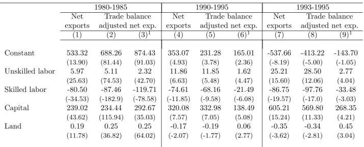
Table 2 presents the results. Columns (1), (4) and (7) show the results when net exports is used as independent variable, whereas in the other columns the independent variable is net exports adjusted by trade balance. The results with adjusted net exports are very similar to those using plain net exports, as seen by the comparison of the results in columns (1), (4) and (7) to those in columns (2), (5) and (8), respectively.
In contrast, the adjustment of the input requirement matrices to technologi-cal changes does alter the results considerably. Columns (3), (6) and (9) present the results. For the period 1980-1985, the results in columns (2) and (3) have all the same sign, but, except from land, they are statistically different. For 1990-1995, all coefficients in columns (5) and (6) are statistically distinct: they all have a larger magnitude for the regression using the observed input requirement matrices, compared to the one using the adjusted input requirements. More-over, when the observed input requirement matrix is used (column (5)), land presents a negative coefficient, but it turns positive when the input requirement matrix is adjusted for technological changes (column (6)). A similar pattern is found in the results for the 1993-1995 period (see columns (8) and (9)).10
Comparing columns (2) and (3) we see that the estimated coefficients are broadly consistent with technological innovations estimations of Table 1, where there was productivity growth biased towards skilled labor and capital, and a decrease in productivity with respect to unskilled labor and land between 1980 and 1990. From eq.(7), the estimated coefficient using the observed data should beunderestimated compared to the adjusted data for the factors which presented productivitygrowth, andoverestimated for the factors for which pro-ductivity have decreased. This is precisely what happens in our estimations: the coefficients for unskilled labor and land are overestimated (although not statistically significantly so for land) and underestimated (in absolute terms) for skilled labor and capital.
The results are also consistent for the trade liberalization periods, which can be seen by comparing columns (5) and (8), to columns (6) and (9), respec-tively. Notice that the adjusted data in this case reproduces the productivity pattern in the first year, 1990. It means that the adjusted datalowers the pro-ductivity of production factors presenting propro-ductivitygrowth over the period. Hence, according to eq.(7), the estimated coefficient will now beoverestimated
in observed data compared to the adjusted one for factors whose productivity
increased. The converse is true for production factors presenting productivity decline over the period.
10
Table 2: Factor Intensity Regressions
1980-1985 1990-1995 1993-1995
Net Trade balance Net Trade balance Net Trade balance
exports adjusted net exp. exports adjusted net exp. exports adjusted net exp.
(1) (2) (3)1 (4) (5) (6)1 (7) (8) (9)1
Constant 533.32 688.26 874.43 353.07 231.28 165.01 -537.66 -413.22 -143.70
(13.90) (81.44) (91.03) (4.93) (3.78) (2.36) (-8.19) (-5.00) (-1.05)
Unskilled labor 5.97 5.11 2.32 11.86 11.85 1.62 25.21 28.50 2.77
(25.63) (74.53) (42.70) (6.63) (5.48) (4.47) (15.60) (12.06) (4.04)
Skilled labor -80.50 -87.46 -119.71 -74.61 -68.16 -21.49 -86.75 -97.76 -33.48
(-34.53) (-182.9) (-78.58) (-11.85) (-9.58) (-6.08) (-19.57) (-17.0) (-3.03)
Capital 239.02 234.44 292.67 320.08 332.98 138.49 605.21 569.80 268.35
(43.62) (115.94) (35.03) (7.57) (7.05) (5.08) (15.24) (11.33) (4.21)
Land 0.19 0.25 0.25 -0.17 -0.19 0.06 -0.35 -0.34 0.45
(11.78) (36.82) (64.02) (-2.07) (-1.77) (2.77) (-3.62) (-2.81) (3.04)
Wald test: null hypothesis that the estimated coefficient is the same as the one from 1980-1985 (the null hypothesis is rejected at 5% when the value is lower than 0.05)
Unskilled labor 0.00 0.00 0.91 0.00 0.00 0.51
Skilled labor 0.74 0.00 0.00 0.16 0.07 0.00
Capital 0.00 0.03 0.20 0.00 0.00 0.70
Land 0.00 0.00 0.00 0.00 0.00 0.18
Number of obs. 100 100 100 300 300 300 300 300 300
1Regression with data adjusted by technological changes.
Notes: (a) All independent variables are measured as a share of the output. (b) t-statistics are in parenthesis. (c) All regressions were estimated using generalized least squares, corrected by heteroscedasticity
and serial autocorrelation of errors.
From the results in Table 1, between 1991 and 1995 there was an increase in productivity towards unskilled labor and capital, accompanied by a productivity decrease in the use of land. No significant productivity change was observed for skilled labor. From the results in Table 2, we see that all coefficients were overestimated with observed data, except the one for land. In fact, the coefficient is negative with observed data, and it turns positive with adjusted data. It means that the lack of comparative advantage in land observed after trade liberalization was due to its lower productivity. It is not attributable neither to a relatively lower land endowment over the period nor to trade liberalization itself.
Table 2 shows also that the coefficients from the regression for the periods 1990-1995 and 1993-1995 are statistically different when the data is not adjusted by technological changes, that is, comparing the results in columns (5) and (8). Using the input-output matrices adjusted by technological changes, the results for these two periods become statistically similar, except for the coefficient for land, which is statistically larger in column (9), compared to column (6).
The regressions reported in columns (3), (6) and (9) present interesting results about the sources of comparative advantages in Brazil before and after trade liberalization. First, the hypothesis that Brazil has comparative advantage in unskilled labor is supported by the results for the two time periods: the coefficient of unskilled labor are positive and statistically significant at 1% level. The Wald test, presented in the bottom of the table, indicates no significative change in the coefficients before and after trade liberalization.
The results confirm the lack of comparative advantage in skilled labor, as the coefficients for that input are negative. The Wald test identifies a signifi-cant change of the coefficient after trade liberalization: the coefficients become smaller in absolute value. This indicates that the comparative ‘disadvantage’ in that factor is less intense in the later period.
The results also indicate that Brazil is relatively abundant in capital, with no significant change across periods, according to the Wald test. This result contradicts the common sense. Given the stage of development of the Brazilian economy, one would not expect the country to relatively abundant in capital, compared to the rest of the world. It may be the case that Brazil is really relatively abundant in capital relative to the world as a whole, keeping in mind that there are many countries at lower stages of development. Alternatively, the country may actually be capital scarce, but this trade pattern resulted from the restrictive trade policies that distorted Brazilian international trade until the late 1980’s. A study of a more recent period should help to check this latter alternative.
4.3
Factor Content in Trade
We complete our analysis with the direct computation of the factor content in international trade. In the results presented in this section, the factor content of trade was computed for all goods, not only those from the industrial sector, as it was the case for factor abundance regressions.11 We computed the factor
abundance both as theconsumptionshare of world factor endowments, indicated in relation (13), and as theincome share of world factor endowments, specified in relation (14).
1. Factor abundance relative to domestic share of world consumption
1980 1985 1990 1995
Factor content in net exports (fT i)
Unskilled labor 1,201,840 3,058,382 1,370,450 315,299
Skilled labor -107,529 317,596 162,329 -182,861
Capital1 -292 42,108 27,377 1,143
Land2 23,815,662 39,231,454 16,647,402 9,449,813
Factor content in value added minus factor content in consumption (fi−ci)
Unskilled labor 1,201,840 3,058,408 1,370,450 315,300
Skilled labor -107,529 317,604 162,329 -182,861
Capital1 -292 42,109 27,377 1,143
Land2 23,815,660 39,231,260 16,647,410 9,449,820
2. Factor abundance relative to domestic share of world income
1980 1985 1990 1995
Factor content in net exports, adjusted by trade balance (fB T i)
Unskilled labor 1,679,887 1,367,219 957,814 2,297,234
Skilled labor -14,141 -52,929 43,944 442,330
Capital1 2,124 30,572 24,732 13,215
Land2 27,538,432 27,373,283 13,804,737 22,660,085
Factor content in value added minus factor content in consumption (fi−cBi )
Unskilled labor 1,679,887 1,367,245 957,814 2,297,234
Skilled labor -14,141 -52,922 43,944 442,330
Capital 2,124 30,573 24,732 13,215
Land2 27,538,430 27,373,080 13,804,740 22,660,090
1R$ 000 from 08/94
2ha
Table 3: Factor Content in Trade
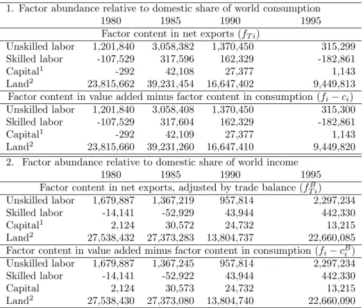
The first set of results in Table 3 presents the factor abundance computations corresponding relations (13), whereas the second set corresponds to relations (14). For each set of results, the left hand side of the relation is presented in the first four rows, and the right hand side on the next four. Hence, the signs of the first four rows have to match the signs of their corresponding lines in the
11
next four rows.
The results reported in Table 3 indicate that Brazil is abundant in unskilled labor and land, with respect to the Brazilian consumption and income shares of world endowments of those factors. The same is true for capital, except for 1980, when the country shows up to be relatively scarce in that factor with respect of the consumption share. As for skilled labor, it presents a positive sign for some years and negative for others, and some signs differ depending on whether consumption or income share is used.
The change of sign of skilled labor content in trade over time is quite peculiar. It is hard to believe that Brazil was relatively scarce in skilled labor in 1980 and 1995, and relatively abundant in the other years, as the results from its content on net exports indicate. It is possible that short run shocks, that affects employment and production, or technological changes not directly accounted for, or even measurement errors, may be biasing the results. Such distortion are, to some degree, taken into account in the regression of factor intensities using panel data.
The factor intensity regressions presented in the previous section indicate that Brazil as being relatively abundant in unskilled labor, capital and land. These results are consistent with the factor abundance test through the direct computation of the factor content in trade presented in Table 3. For skilled labor, the factor intensity regressions reveal relative scarcity, which is corrobo-rated by the factor content test only for some of the years studied.
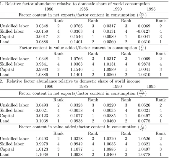
We also measure the factor content in trade and endowments as a share of factor services content in domestic consumption. This allows us to use eq.(15) for net exports and (16) for net exports adjusted by trade balance, and rank factors according to its relative abundance, as revealed by international trade. Table 4 presents the results.
In all cases, skilled labor is in fourth place, that is, it is the least abundant factor of production in Brazil. This result is consistent with the econometric results in section 4.2. It is interesting to note that the ranking of the inputs is the same in the first and last years, 1980 and 1995, and somewhat different from 1985 and 1990. Unskilled labor is never in first place. It ranks in second place in 1980 and 1995, and in third for the other years. Capital alternates between third place in the first and last years, and first in the other years. Finally, land is in first place in 1980 and 1995, and second in the others.
The results from the factor intensity regressions, presented in Table 2, and from the factor content in trade, in Table 4, picture Brazil as relatively abundant in capital and land, in relation to labor in general.
5
Conclusions
Table 4: Relative Factor Content in Trade
1. Relative factor abundance relative to domestic share of world consumption
1980 1985 1990 1995
Factor content in net exports/factor content in consumption (fT i
ci )
Rank Rank Rank Rank
Unskilled labor 0.0348 2 0.0766 3 0.0317 3 0.0069 2
Skilled labor -0.0159 4 0.0363 4 0.0131 4 -0.0127 4
Capital -0.0017 3 0.1546 1 0.0989 1 0.0041 3
Land 0.0886 1 0.1401 2 0.0560 2 0.0310 1
Factor content in value added/factor content in consumption (fi
ci)
Rank Rank Rank Rank
Unskilled labor 1.0348 2 1.0766 3 1.0317 3 1.0069 2
Skilled labor 0.9841 4 1.0363 4 1.0131 4 0.9873 4
Capital 0.9983 3 1.1546 1 1.0989 1 1.0041 3
Land 1.0886 1 1.1401 2 1.0560 2 1.0310 1
2. Relative factor abundance relative to domestic share of world income
1980 1985 1990 1995
Factor content in net exports/factor content in consumption (fT iB
cB i )
Rank Rank Rank Rank
Unskilled labor 0.0493 2 0.0328 3 0.0220 3 0.0526 2
Skilled labor -0.0021 4 -0.0058 4 0.0035 4 0.0321 4
Capital 0.0123 3 0.1077 1 0.0885 1 0.0497 3
Land 0.1038 1 0.0938 2 0.0460 2 0.0778 1
Factor content in value added/factor content in consumption (fi
cB i )
Rank Rank Rank Rank
Unskilled labor 1.0493 2 1.0328 3 1.0220 3 1.0526 2
Skilled labor 0.9979 4 0.9942 4 1.0035 4 1.0321 4
Capital 1.0123 3 1.1077 1 1.0885 1 1.0497 3
and taken into account in the factor abundance tests. They turned out to be significant.
Two approaches were used to inspect relative factor abundance in Brazil. We estimated factor intensity regressions on net exports and we computed directly the factor content in international trade. The results from the two approaches are compatible.
According to our results, Brazilian international trade reveals comparative advantages in the use of unskilled labor, in capital and in land, and no compar-ative advantage in the use of skilled labor. The same pattern of comparcompar-ative advantage is observed before and after trade liberalization.
6
References
References
[1] Aw, B-Y. (1983),“The Interpretation of Cross-Section Regression Test of
The Heckscher-Ohlin Theorem with Many Good and Factors,” Journal of
International Economics 14(1-2):163-167.
[2] Baldwin, R. E. (1971),“Determinants of the Commodity Structure of U.S.
Trade,” American Economic Review 61 (1): 126-46.
[3] Bonelli R. and R. Fonseca (1998), “Ganhos de Produtividade e de
Eficiˆencia: Novos Resultados para a Economia Brasileira,” Pesquisa e
Planejamento Econˆomico 28(2): .
[4] Bowen, P. H. and L. Sveikauskas (1992), “Judging Factor Abundance,”
Quarterly Journal of Economics 107(2): 599 - 620.
[5] Bowen, P. H., E. E. Leamer and L. Sveikasukas (1987), “Multicountry,
Multifactor Tests of the Factor Abundance Theory.” American Economic
Review 77(5): 791-809.
[6] Branson, H. W. and N. Monoyios (1977), “Factor Inputs in U.S. Trade,”
Journal of International Economics 7(2): 111-31.
[7] Brecher, R.A. and E.U.Choudhri (1981), “The Leontief Paradox: Contin-ued,”Journal of Political Economy 90(4): 820-3.
[8] Davis, P.A and D. E. Weinstein (1998), “An Account of Global Factor Trade,” National Bureau of Economic Research, Working Paper # 6785.
[9] Gonzaga, G., N. Menezes-Filho, and C. Terra (2002), “Trade Liberaliza-tion and EvoluLiberaliza-tion of Skill Earnings Differentials in Brazil,” Journal of International Economics 68(2): 345-367.
[11] Harkness, J. (1978), “Factor Abundance and Comparative Advantage,”
American Economic Review 68(5): 784-800.
[12] Kahn, J.A. and J.-S. Lim (1998), “Skilled Labor-Augmenting Technical Progress in U.S. Manufacturing,”Quarterly Journal of Economics 113(4): 1281-308.
[13] Leamer, E. E. (1980), “The Leontief Paradox Reconsidered,”The Journal of Political Economy 88(3): 495-503.
[14] Leamer, E. E. and H. P. Bowen (1981), “Cross-Section Test of the
Heckscher-Ohlin Theorem: Comment,”American Economic Review 71(5):
1040-43.
[15] ...(1996), “In Search of the Stolper-Samuelson Effects on US Wages,” NBER Working Paper # 5427.
[16] Leontief, W. W. (1953), “Domestic Production and Foreign Trade: The American Capital Position Re-examined,” Economia Internazionale, 7(1):3-32. Reprinted in R. E. Caves and H. G. Johnson (eds.)Readings in Inter-national Economics,Richard D. Irwin, ICB, 1968.
[17] Maskus, E. K. (1983), “Evidence on Shifts in the Determinants of the Struc-ture of U.S. Manufacturing Foreign Trade, 1958-76,”Review of Economics and Statistics 65(3): 415-422.
[18] Muendler, M. A. (2001), “The Pesquisa Industrial Anual 1986-1998: A Detective’s Report,” IBGE, Rio de Janeiro, mimeo.
[19] Muriel, H. B. (2004),Trˆes ensaios sobre as predi¸c˜oes de Heckscher-Ohlin: Quest˜oes te´oricas e testes emp´ıricos, PhD. Thesis PUC-Rio.
[20] Ramazani, R.M. and K.E.Markus (1993), “A Test of Factor Endowments Model of Trade in a Rapidly Industrializing Country: The Case of Korea,”
The Review of Economics and Statistics 74(3): 568-72.
[21] Ferreira, P.C. and J. L. Rossi (2003), “New Evidence from Brazil on Trade Liberalization and Productivity Growth,” International Economic Review
44(4): 1383–1405.
[22] Stern, R.M. and K.Markus (1981). “Determinants of the Structure of U.S. Foreign Trade, 1958-76,” Journal of International Economics 11(2): 207-24.
[23] Trefler, D. (1993), “International Factor Price Differences: Leontief was Right,”Journal of Political Economy 101(6): 961-87.
[24] ... (1995), “The Case of the Missing Trade and Other Mysteries,”
American Economic Review 85(5): 1029-46.
[25] Trefler, D. and S. Chun Zhu (2000), “Beyond the Algebra of Explanation