Implied Volatility Smirk in L´evy Markets
April 7, 2016
Abstract
We introduce skewed L´evy models, characterized by a symmetric jump measure multiplied by dumping exponential factor. This models exhibit a clear implied volatility pattern, where the dumping param-eter controls the skew of the implied volatility curve, resulting in a measure of the skewness of the model. We show that the variation of this parameter produces the typical smirk observed in implied volatil-ity curves. Some theoretical facts supporting this findings are proved, and some open questions are posed.
Keywords: Skewness; L´evy Processes; Implied volatility Smirk.
JEL Classification: C52; G10
1
Introduction
On the other hand, there is a is well-established relationship between the symmetry of the implied volatility and the market symmetry, which is equivalent to the put-call symmetry. This has been derived by Fajardo and Mordecki [2006] and Carr and Lee [2009] for L´evy process and local and stochastic volatility models respectively. Also, Fajardo and Mordecki [2014] showed the relationship between the skewness premium and the market symmetry parameter.
In this paper focusing on a subclass of L´evy processes, where exponen-tial dampening controls the skewness, we use duality techniques to obtain a result that allows us to relate the implied volatility skew with a market skewness parameter. Although, more general processes have been studied in the literature which include stochastic volatility models, we focus on a par-ticular class. For this class we get a deeper insight into how this parpar-ticular process generates the skew. More exactly, there is an intrinsic relationship between the market skewness parameter and the risk neutral excess of kurto-sis, which will allow us to relate the risk neutral skewness and kurtosis with the implied volatility skew. The main result obtained shows that all skewed models with continuous density have a positive cross partial derivative w.r.t.
x (the log-moneyness) and β at the point x = 0 and β = −1/2, giving, as a consecuence, a precise monotonicity behavior of the implied volatility in a neighborhood of this point.
The paper is organized as follows. In Section 2 we introduce the model. In Section 3, through put-call duality, we obtain a symmetry property of the implied volatility which extends the result obtained by Fajardo and Mordecki [2006]. In Section 4 we obtain our main result. In Section 5 we analyze our finding across different models, and present a complementary example that shows that the obtained monotonicity behavior can not be extended beyond a certain neighborhood. The last section concludes.
2
The Model
Consider a real valued stochastic process X ={Xt}t≥0, defined on a filtered probability space (Ω,F,(F),Q). We assume that the process is adapted, starts at zero, has c`adl`ag paths, and is such that for 0 ≤ s < t the ran-dom variables Xt−Xs are independent of theσ-fieldFs, with a distribution
Skorokhod [1991], Bertoin [1996] or Sato [1999]. For L´evy processes used in financial models see Boyarchenko and Levendorski˘i [2002], Schoutens [2003] or Cont and Tankov [2004].
In order to characterize the law ofXunderQ, consider the L´evy-Khinchine formula, that, for z ∈iR, states
EezXt =etψ(z),
where
ψ(z) = γz+1 2σ
2z2+
Z
R
ezy−1−zh(y)
Π(dy), (1)
withh(y) =y1{|y|<1}, a fixed truncation function,γandσ ≥0 real constants,
and Π a measure on R\ {0}1 such that R
(1∧y2)Π(dy)<∞, called theL´evy
measure. The triplet (γ, σ,Π) is thecharacteristic triplet of the process, and completely determines its law.
By aL´evy market we mean a model for a financial market with two assets: a savings account B, given by the deterministic process:
Bt=ert, t≥0,
for a fixed interest rate r≥0 and a stock S, with price process S ={St}t≥0 modelled by:
St=S0eXt+rt, S0 >0,
where X ={Xt}t≥0 is a L´evy process.
In this approach we assume that the probability measure Q is already the risk neutral martingale measure. In other words, prices for derivatives written on the underlying processS ={St}t≥0 are computed as expectations with respect toQ, and the discounted process{e−rtS
t}t≥0 is aQ-martingale. In terms of the characteristic exponent of the process this means that
ψ(1) = 0, (2)
based on the fact, that Ee−rtS
t = etψ(1) = 1. Observe that, as usual in
fi-nancial modeling with L´evy processes, this requires that the complex funcion
ψ(z) defined in (1) can be extended at least to the strip 0≤Re(z)≤1, what is equivalent to R
y≥1e
yΠ(dy)<∞, condition that we assume in what follows
(see Theorem 25.3 in Sato [1999]). Condition (2) can also be formulated in terms of the characteristic triplet (γ, σ,Π) of the process X as
γ =−σ2/2−
Z
R
ey−1−h(y)
Π(dy). (3)
Consequently
ψ(z) =z(z−1)σ 2
2 +
Z +∞
−∞
[(ezy−1)−z(ey−1)]Π(dy).
2.1
Skewed Models
We are particularly interested in the case where {Xt,Q}has a L´evy measure
which can be represented in the form
Πβ(dy) =eβyΠ0(dy), (4)
where Π0 is a symmetric measure, i.e. Π0(dy) = Π0(−dy). We assume that Π0 does not depend onβ. In this case we denoteQbyQβ. As a consequence,
we study the L´evy process
{Xt,Qβ}t≥0 (5)
with triplet (γβ, σ,Πβ) whereγβ is as in (3) with Π = Πβ and Πβ is as in (4).
In this case, we denote the characteristic exponent by ψβ and we write
ft(x;β) for the density ofXt underQβ, when it exists. For the existence and
smoothness of the density of an infinitely divisible distribution see sections 27 and 28 in Sato [1999].
This parametrization allows us to quantify the smirkness of the model by β+ 1/2, since β =−1/2 gives the symmetry of the implied volatility as a function of the log-moneyness x= logK/F, where K is the strike of a call option and F = S0erT is the corresponding futures price of the underlying asset (see Fajardo and Mordecki [2006]).
3
Put-Call Duality and Implied Volatility.
3.1
Symmetry and Duality of the General Model
Let {Xt,Q} be a general L´evy process as in Section 2 and let dQ˜t =eXtdQt
˜
Qt and Qt are the restrictions of ˜Q and QtoFt respectively. We know that
the triplet (˜γ,σ,˜ Π) of˜ {X˜t} under ˜Q is
˜
γ =−σ2/2−R
R(e
y−1−h(y)) ˜Π(dy)
˜
σ =σ
˜
Π(dy) = e−yΠ(−dy)
(see Fajardo and Mordecki [2006]) and for the option prices
Call(S0, Kx, r, T, ψ) =
Kx
F P ut(S0, K−x, r, T,ψ˜), (6)
where Kx =S0erT+x and F =S0erT (see Fajardo and Mordecki [2014]). From (6) we have the following relation for the implied volatility
σimp(x,Π) =σimp(−x,Π)˜ , (7)
where σimp denotes the implied volatility, that is the volatility parameter
which reproduces the price obtained in the L´evy model if one applies the Black-Scholes formula.
3.2
Symmetry and Duality for Skewed Models
In the case of the skewed model given by (5), we have ˜
ft(x;β) = e−xft(−x;β)
where ˜ft(x;β) denotes the density of the distribution of ˜Xt under ˜Qβ, the
dual of Qβ. Now for β = −1/2 we know that market symmetry property
holds, i.e, the distribution of Xt under Qβ and the distribution of ˜Xt under
˜
Qβ are identical. Form here one gets
ft(x;−1/2) = ˜ft(x;−1/2) =e−xft(−x;−1/2). (8)
In particular for any β, ˜Πβ(dy) = e−(β+1)yΠ0(dy) and we can rewrite relationship (7) in the form
σimp(x, β+ 1/2) =σimp(−x,−(β+ 1/2)). (9)
In Fajardo and Mordecki [2006] this result is obtained for the case β =
−1/2.
x
−0.4
−0.2 0.0
0.2 0.4
beta
−1.5 −1.0 −0.5 0.0 0.5
z
0.26 0.28 0.30 0.32 0.34 0.36
●
Figure 1: Variance Gamma Implied volatility as function of x and β. Other parameters: α= 5, λ = 1, T = 1, r= 0.05.
4
Implied Volatility Behavior in a
Neighbor-hood of
β
=
−
1
/
2
.
In this section we present our main result. We describe the implied volatility behavior in a neighborhood of β =−1/2.
We obtain two results involving the implied volatility. The first one: the implied volatility as a function of β, in a neighborhood of β = −1/2, is increasing whenxis in a right-neighborhood ofx= 0 and is decreasing when
xis in a left-neighborhood ofx= 0. The second one: the implied volatility as a function ofx, in a neighborhood ofx= 0, is increasing whenβis in a right-neighborhood of −1/2 and it is decreasing when β is in a left-neighborhood of −1/2.
In order to formulate the following results, write the Black-Scholes for-mula in terms of x as
where
d1 =−
x+σ2
imp(x, β)T2
σimp(x, β)
√
T and d2 =
−x−σ2
imp(x, β)T2
σimp(x, β)
√
T .
Now, differentiating with respect tox, we obtain
∂BS(Kx, σimp(x, β))
∂x =
∂BS(Kx, σimp)
∂Kx
∂Kx
∂x +
∂BS(Kx, σimp)
∂σimp
∂σimp(x, β)
∂x
=−S0exN(d2) +
√
T φ(d1)
∂σimp(x, β)
∂x .
where N and φ denote the standard normal cdf and density, respectively. On the other hand, the value of a call option under the L´evy process (5) is denoted by V, and given by
V(x, β) =e−rT Eβ(ST −Kx)+=S0
Z +∞
x
(ey−ex)dQβ. (10)
In order to obtain the differentiability of the implied volatility with re-spect to x, we need the differentiability of the function V(x, β) with respect to x. In view of (10), the existence of a continuous density of the mea-sure Qβ is a sufficient condition for the differentiability of V. According to Proposition 28.1 in Sato [1999], the condition
Z
R|
etψβ(iz)
|dz <∞ (11)
implies the existence of a continuous density. Throughout this section we assume that condition (11) holds. We then have
∂V(x, β)
∂x =−S0e
xQ
β(XT > x),
and from the equalityBS(Kx, σimp(x, β)) =V(x, β), we obtain
∂σimp(x, β)
∂x = S0ex
N(d2)−Qβ(XT > x)
φ(d1)
√
T =S0
N(d2)−Qβ(XT > x)
φ(d2)
√
T .
(12)
Theorem 1. For any maturity T, if {Xt,Qβ} is a skewed model with
con-tinuous density, then
1. there exists ε >0 such that:
(a) if β ∈(−12 −ε;−12) then ∂σimp(0, β)
∂x <0,
(b) if β ∈(−12;−21 +ε) then ∂σimp(0, β)
∂x >0.
2. There exists ε >0 such that:
(a) if x∈(0, ε), then ∂σimp(x,−1/2)
∂β >0,
(b) if x∈(−ε,0), then ∂σimp(x,−1/2)
∂β <0.
For the proof of Theorem 1 we introduce some previous results.
Proposition 1. Let {Xt,Qβ} a skewed model. Then,
ψβ(z) =ψ0(z+β)−ψ0(β)−zµβ,
where µβ =βσ2+
R
R(e
y−1)(eβy−1)Π
0(dy).
If there exists continuous density we have
ft(x;β) = eβ x+tµβ
−tψ0(β)
ft(x+tµβ; 0),
Proof. We define the measure ˆQ such that
dQˆ
dQ0
=eβXt−tψ0(β)
. (13)
Then, from the Esscher transform,{Xt,Qˆ}is a L´evy process with triplet
(ˆγ, σ, eβyΠ
0(dy)) with ˆγ =βσ2+γ0+
R
R(e
βy −1)h(y)Π
0(dy).
We observe that{Xt,Qˆ}and{Xt,Qβ}are both L´evy processes that differ
only in the drift term, therefore
{Xt,Qβ}
L
where µβ =βσ2+γ0−γβ +
R
R(e
βy−1)h(y)Π
0(dy). From (13) and (14) we obtain:
Eβ(ezXt) =ˆE(ez[Xt−tµβ]) =E0(e(z+β)Xt−t[ψ0(β)+zµβ]), (15)
and from (15) the result follows.
On the other hand, if a continuous density exists we have
ft(x;β) =
1 2π
Z
R
e−izxetψβ(iz)dz
= 1 2π
Z
R
e−izxet[ψ0(iz+β)−ψ0(β)−izµβ]dz
=e−tψ0(β) 1
2π Z
R
e−iz(x+tµβ)etψ0(iz+β)
dz
=e−tψ0(β) 1
2π Z
R
e−(iw−β)(x+tµβ)etψ0(iw)
dw
=eβ(x+tµβ)−tψ0(β) 1
2π Z
R
e−iw(x+tµβ)etψ0(iw)
dw
=eβ(x+tµβ)−tψ0(β)
ft(x+tµβ; 0).
We observe that for β = 0 in (5), the process Xt − tγ0 is symmetric because of the symmetry of the jump measure. If there exists a density, we have
ft(x+tγ0; 0) =ft(−x+tγ0; 0).
Corollary 1. If {Xt,Qβ} is a skewed model with continuous density, then
ft(x;−1/2)≤ft(0;−1/2)e−1/2x ∀x∈R.
Proof. Observe that
µ−1/2 =−σ2/2 +γ0−γ−1/2+
Z
R
h(y)(e−y/2−1)Π0(dy)
=γ0+
Z
R
because (ey −1)e−y/2−h(y) is a odd function. On the other hand,
ft(x+tγ0; 0) = 1 2π
Z
R
e−iz(x+tγ0)
etψβ(iz)dz
= 1 2π
Z
R
e−izxet[−izγ0+ψβ(iz)]dz
= 1 2π
Z
R
cos(zx)et[−izγ0+ψ0(iz)]
dz (17)
≤ 1
2π Z
R
et[−izγ0+ψ0(iz)]
dz
=ft(tγ0; 0), (18)
where in (17) we use that the imaginary part of−izγ0+ψ0(iz) =−z2σ2/2 +
R
R(e
izy−1−izh(y))Π
0(dy) vanishes. From Proposition 1 and (16) we have
ft(x;−1/2) =e−1/2(x+tγ0)−tψ0(−1/2)ft(x+tγ0; 0)
=ft(0;−1/2)e−x/2
ft(x+tγ0; 0)
ft(tγ0; 0)
. (19)
Observe that from (18),ft(tγ0; 0)6= 0. From (18) and (19) we obtain the result.
Lemma 1. If {Xt,Qβ} is a skewed model with continuous density, then
∂Qβ(Xt >0)
∂β
−1/2 <0
Proof. For simplicity, we denote ft(y) := ft(y;−1/2), the density of the
distribution of Xt at β = −1/2. From the Lewis formula for a digital call
option (see Lewis [2001]), for some 0< v < 1, we have
Qβ(Xt> x) =−
1 2π
Z
iv+R
Then, differentiating with respect toβ we obtain
∂Qβ(Xt >0)
∂β
−1/2 =− t
2π Z
iv+R
etψβ(−iz) iz
∂ψβ(−iz)
∂β
−1/2dz
=− t 2π
Z
iv+R
etψβ(−iz) iz
hZ
R
e−izy −1 +iz(ey−1)
ye−y/2Π0(dy)
i
dz (20)
=t Z
R
ye−y/2hQ−1/2(Xt>−y)−Q−1/2(Xt >0)−(ey−1)ft(0)
i
Π0(dy)
(21)
=t Z +∞
0
ye−y/2hQ−1/2(Xt >−y)−Q−1/2(Xt >0)−(ey−1)ft(0)
i
Π0(dy)
−t Z +∞
0
yey/2hQ−1/2(Xt> y)−Q−1/2(Xt>0)−(e−y −1)ft(0)
i
Π0(dy)
(22)
=t Z +∞
0
ye−y/2hQ−1/2(−y < Xt <0)−(ey−1)ft(0)
i
Π0(dy)
−t Z +∞
0
yey/2h−Q
−1/2(0< Xt < y)−(e−y−1)ft(0)
i
Π0(dy)
=t Z +∞
0
ye−y/2hQ−1/2(−y < Xt <0) +eyQ−1/2(0< Xt < y)
−2(ey−1)ft(0)
i
Π0(dy),
where in (20) we use that Π0 does not depend onβ, in (21) we use the Fubini Theorem and in (22) we use the symmetry property of Π0.
Letg(y) :=Q−1/2(−y < Xt<0) +eyQ−1/2(0< Xt < y)−2(ey−1)ft(0).
From (8), we have that
g′(y) =f
t(−y) +eyQ−1/2(0< Xt< y) +eyft(y)−2eyft(0)
=eyhQ−1/2(0< Xt< y) + 2[ft(y)−ft(0)]
i
From Corollary 1 and (23) we have
e−yg′(y) =
Z y
0
ft(s)ds+ 2[ft(y)−ft(0)]
≤ft(0)
Z y
0
e−1/2sds+ 2[ft(y)−ft(0)]
=−2ft(0)e−1/2y+ 2ft(y)≤0.
Observe thatft(0)e−1/2y cannot be equal toft(y) for everyy >0 because
in these case, from (8), we get the absurd ft(−y) = ft(0)e1/2y for y > 0.
Then, there exist an open interval I ⊂R+ such that g′(y)<0 fory∈I.
Since g is decreasing, g(y)≤ g(0) = 0 for y >0 and g(y) <0 for y ∈ I, this implies
∂Qβ(Xt>0)
∂β
−1/2 =t
Z +∞
0
ye−y/2g(y)Π0(dy)<0.
Proof of Theorem 1. From (12) we obtain:
∂2σ
imp(x, β)
∂β∂x = ∂ ∂β
∂σimp(x, β)
∂x
=S0
[φ(d2)∂d∂β2 −
∂Qβ(XT>x)
∂β ]−[N(d2)−Qβ(XT > x)](−d2) ∂d2
∂β
φ(d2)
√
T .
We observe that
∂d2
∂β =−
T3/2σ2
imp(x, β)
∂σimp(x,β)
∂β −(x+σ
2
imp(x, β)T2)
∂σimp(x,β)
∂β
σ2
imp(x, β)T
.
From (9), we have∂βσimp(0,−1/2) = 0 and then∂βd2(0,−1/2) = 0 where we conclude that, from Lemma 1
∂2σ
imp(0,−1/2)
∂β∂x =−
S0
φ σimp(0,−1/2)
√
T
2
√ T
∂Qβ(XT >0)
∂β
From (24) we have
∂ ∂β
∂σimp(0, β)
∂x
−1/2 >0,
then, there exists ε > 0 such that ∂xσimp(0, β) is increasing as a function
of β ∈ (−12 − ε;−12 + ε). The results 1(a) and 1(b) are obtained from
∂xσimp(0,−1/2) = 0.
Now we prove 2(a). The result 2(b) is obtained from the implied volatility symmetry (9).
Under regularity conditions we have ∂2σimp(x,β)
∂β∂x = ∂2
σimp(x,β)
∂x∂β , then from
(24) we have
∂ ∂x
∂σimp
∂β (0,−1/2) = ∂2σ
imp(0,−1/2)
∂x∂β >0. (25)
From (25) and the symmetry (9) we have that there exists ε > 0 such that, if x∈(0, ε) then
∂σimp
∂β (x,−1/2)> ∂σimp
∂β (0,−1/2) = 0.
This conclude the proof of the Theorem.
5
Examples
We discuss the applicability of our Theorem to infinite activity models, jump-diffusion models and show a complementary example that shows why the obtained monotonicity results of the implied volatility is only local.
5.1
Infinite Activity Models.
The Generalized Hyperbolic (GH), including the Variance Gamma (VG) and Normal Inverse Gaussian (NIG) and the Meixner models, are skewed, as follows from Fajardo and Mordecki [2006]. Particular instances of the CGMY model is also skewed (see Fajardo and Mordecki [2006]). As they all have a continuous density, they verify the hypothesis of Theorem 1.
-0.6 -0.4 -0.2 0.0 0.2 0.4 0.6
0.45
0.55
-0.6 -0.4 -0.2 0.0 0.2 0.4 0.6
0.45
0.55
-0.6 -0.4 -0.2 0.0 0.2 0.4 0.6
0.45
0.55
-0.6 -0.4 -0.2 0.0 0.2 0.4 0.6
0.45
0.55
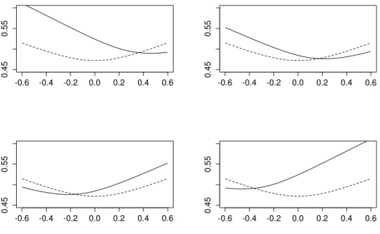
Figure 2: Variance Gamma implied volatility in terms of x. Doted line
β = −0.5. Continuous line: top left β = −1.5, top right β = −1, bottom left β = 0, bottom right β = 0.5. Other parameters: α = 4, λ = 2, T = 1,
r = 0.05.
5.2
Jump-Diffusion Models.
Observe that any jump-diffusion model with positive diffusion component (σ >0) has a differentiable density of any order (use Theorem 4 V.4 in Feller [1971] and Theorem 2.27 in Folland [1999]).
The Merton model has a L´evy measure of the type Π(dy) = eβyΠ
0(dy) with Π0 symmetric, but depending on β:
Π(dy) =λ√ 1
2πσJ
exp
(
−12
y−µJ
σJ
2) dy
=λe−
1 2(
µJ σJ)
2
eβy√ 1
2πσJ
exp
− y
2
2σ2
J
whereβ =µJ/σ2J andµJ depends onβ. For this reason we adapt the Merton
model re-parameterizing its L´evy measure.
Definition 1 (Skewed Merton model). We define the Skewed Merton model
as a L´evy process with triplet (γ, σ,Π(dy)), where
Π(dy) =λeβy√ 1
2πσJ
exp
− y
2
2σ2
J
dy.
In Figure 3 we show the behavior of the implied volatility in a neighbor-hood of β =−1/2.
−0.4 −0.2 0.0 0.2 0.4
0.340
0.345
0.350
0.355
x=log(K/F)
Figure 3: Skewed Merton Implied volatility with: T = 1, r = 0.05, σ = 0.2,
λ = 2, σJ = 0.2. Continuous line β = −0.5, dotted line: β = −.6, dashed
line: β =−.4.
The Kou model has a jump density given byg(y) =pθ1eθ1y1{y≤0}+ (1−
p)θ2e−θ2y1{y>0}, where p ∈ (0,1) and θ1, θ2 > 0. The following particular case constitutes a skewed model.
Definition 2 (Skewed Kou Model). We define the Skewed Kou model as a L´evy process with triplet (γ, σ,Π(dy)), where
Π(dy) = λeβy−α|y|dy.
5.3
A Complementary Example.
In this section we show an example of a L´evy process where the corresponding model verifies the regularity conditions of Theorem 1, but does not verify
∂σimp(0, β)/∂β > 0 for all β > −1/2 neither ∂σimp(x,−1/2)/∂β > 0 for all
x >0.
Definition 3 (Diffusion with a two-sided Poisson jump process). We define the diffusion with a two-sided Poisson jump process as a L´evy process where the jump measure is given by
Πβ(dy) =λeβy
δa(y) +δ−a(y)
dy.
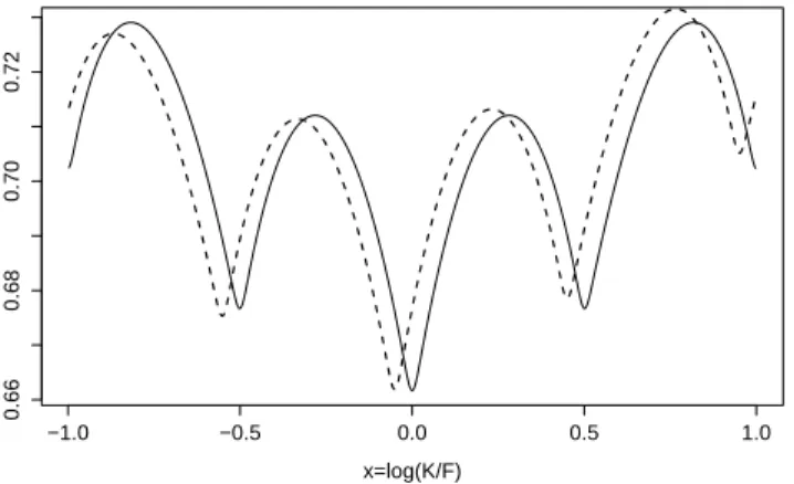
If the diffusion with a two-sided Poisson jump process has positive diffu-sion part, then it verify the Theorem 1. However ,we show in Figure 5 that
∂xσimp(0, β) is not positive, neither negative2 for all β >−1/2. And we show
in Figure 4 that σimp has local minima at x = a and x = −a, where the
results of Theorem 1 cannot be extended to the entire real line.
It is clear that this setting is not interesting as a realistic model, however it is a important example when we try to derive results on implied volatility in the context of L´evy process.
2Observe that here we consider any maturity, in contrast with the results obtained in
−1.0 −0.5 0.0 0.5 1.0
0.66
0.68
0.70
0.72
x=log(K/F)
Figure 4: Implied Volatility under diffusion with a two-sided Poisson jump process with σ = 0.01, a = 0.5 and λ = 2. Continuous line: β = −0.5, dashed line: β =−0.4.
−0.4 −0.2 0.0 0.2 0.4
0.135
0.140
0.145
0.150
0.155
0.160
Figure 5: Implied Volatility under diffusion with a two-sided Poisson jump process with σ = 0.01, a= 0.1 λ= 2, T = 1 and r = 0.05. Continuous line:
β =−0.5, doted line: β = 1 and dashed line: β = 3.
6
Conclusions
depends on a parameter β. This parameter quantifies the skewness of the model, and its variation captures the typical smirk feature observed in im-plied volatility curves. Our main result (see Theorem 1) shows that skewed models with continuous density exhibit a precise monotonicity behavior of the implied volatility surface, as a function of the log-moneyness and the skewness parameter. These results are independent of the maturity of the options, and apply to many main models in the literature. Other popular models can be easily adapted to be skewed. Finally, we present a simple ex-ample that shows that the obtained monotonicity behavior can not be further extended.
Our proposal establishes a link between the visual analysis of the im-plied volatility curves and its mathematical modelling, through the skewness parameter β. It also raises several questions regarding the other second derivatives of the implied volatility surface.
References
J. Bertoin. L´evy Processes. Cambridge University Press, Cambridge, 1996.
F. Black and M. Scholes. The Pricing of Options and Corporate Liabilities.
Journal of Political Economy, 81:637–659, 1973.
S. Boyarchenko and S. Levendorski˘i. Non-Gaussian Merton-Black-Scholes Theory. World Scientific, River Edge, NJ, 2002.
P. Carr and R. Lee. Put Call Symmetry: Extensions and Applications. Math. Finance., 19(4):523–560, 2009.
P. Carr and L. Wu. Finite Moment Log Stable Process and Option Pricing.
Journal of Finance, 58(2):753–777, 2003.
R. Cont and P. Tankov. Financial Modelling with Jump Processes. Chapman & Hall /CRC Financial Mathematics Series, 2004.
J. Fajardo and E. Mordecki. Symmetry and Duality in L´evy Markets. Quan-titative Finance, 6(3):219–227, 2006.
W. Feller. An introduction to probability theory and its applications. Vol. II.
Second edition. John Wiley & Sons Inc., New York, 1971.
G. Folland. Real analysis: modern techniques and their applications. Pure and applied mathematics. Wiley, 1999. ISBN 9780471317166.
S. Foresi and L. Wu. Crash-O-Phobia: A Domestic Fear or A Worldwide Concern? Journal of Derivatives, 13(2), 2005.
S. Gerhold and I. C. G¨ul¨um. The Small-Maturity Implied Volatility Slope for L´evy Models. Preprint, available at http://arxiv.org/abs/1310.3061, 2014.
J. Jacod and A. Shiryaev. Limit Theorems for Stochastic Processes. Springer, Berlin, Heidelberg, 1987.
A. L. Lewis. A Simple Option Formula for General Jump-diffusion and Other Exponential L´evy processes. Working paper. Envision Financial Systems and OptionCity.net Newport Beach, California. Available at http://www.optioncity.net, 2001.
K.-I. Sato. L´evy Processes and Infinitely Divisible Distributions. Cambridge University Press, Cambridge., 1999.
W. Schoutens. L´evy Processes in Finance: Pricing Financial Derivatives. Wiley, New York, 2003.