Analysing movements in investor’s risk aversion
using the Heston volatility model
Alexie ALUPOAIEI The Bucharest University of Economic Studies [email protected] Andrei HREBENCIUC The Bucharest University of Economic Studies
[email protected] Ana-Maria SĂNDICĂ The Bucharest University of Economic Studies
Abstract. In this paper we intend to identify and analyze, if it is the case, an “epidemiological” relationship between forecasts of professional investors and short-term developments in the EUR/RON exchange rate. Even that we don’t call a typical epidemiological model as those ones used in biology fields of research, we investigated the hypothesis according to which after the Lehman Brothers crash and implicit the generation of the current financial crisis, the forecasts of professional investors pose a significant explanatory power on the futures short-run movements of EUR/RON. How does it work this mechanism? Firstly, the professional forecasters account for the current macro, financial and political states, then they elaborate forecasts. Secondly, based on that forecasts they get positions in the Romanian exchange market for hedging and/or speculation purposes. But their positions incorporate in addition different degrees of uncertainty. In parallel, a part of their anticipations are disseminated to the public via media channels. Since some important movements are viewed within macro, financial or political fields, the positions of profess-sional investors from FX derivative market are activated. The current study represents a first step in that direction of analysis for Romanian case. For the above formulated objectives, in this paper different measures of EUR/RON rate volatility have been estimated and compared with implied volatilities. In a second timeframe we called the co-integration and dynamic correlation based tools in order to investigate the relationship between implied volatility and daily returns of EUR/RON exchange rate.
Keywords: implied volatility; smile volatility; dynamic correlation; error correction model.
1. Introduction
Summing-up all these considerations and based on recently elaborated analyses by Alupoaiei, Codîrlaşu and Săndică (2012), we investigate the case of existing “epidemiological” relationship between forecasts of professional investors and short-term developments in the EUR/RON exchange rate. Even if we don’t call a typical epidemiological model as those ones used in biology fields of research, we investigated the hypothesis according to which after the Lehman Brothers crash and, implicit, the generation of the current financial crisis, the forecasts of professional investors pose a significant explanatory power on the futures short-run movements of EUR/RON. How does it work this mechanism? Firstly, the professional forecasters account for the current macro, financial and political states, then they elaborate forecasts. Secondly, based on that forecasts they get positions in the Romanian exchange market for hedging and/or speculation purposes. But their positions incorporate in addition different degrees of uncertainty. In parallel, a part of their anticipations are disseminated to the public via media channels. Since some important movements are viewed within macro, financial or political fields, the positions of professional investors from FX derivative market are activated. The current study represents a first step in that direction of analysis for Romanian case. For the above formulated objectives, in this paper there have been estimated different measures of EUR/RON rate volatility and compared with implied volatilities. In a second timeframe we called the co-integration and dynamic correlation based tools in order to investigate the relationship between implied volatility and daily returns of EUR/RON exchange rate.
2. Theoretical model
In this section we will briefly present the theoretical background of volatility smile concept of implied, stochastic and conditional volatility. Once we establish a base for the volatility features in Romanian FX market we move further to analyze the co-integration and dynamic correlation in order to investigate the relationship between implied volatility and daily returns of exchange rate.
2.1. Smile volatility
Forward looking financial indicators represents informative predictors of the behaviour of the asset price; therefore those options gained attention in recent years. Neftci (2008) explained how risk reversal represents a measure of the bias in a volatility smile, since a symmetric smile implies that zero cost risk reversal could be achieved.
The measure of an option’s moneyness is called delta, such as at the money (ATM) options have a delta around 50 and the following relationship holds:
σ 5 deltaRR σ 5 deltaput σ 5 deltacall (1) Where σ 5 deltaRR , σ 5 deltacall , σ 5 deltaput represents the implied volatilites of a risk reversal, namely the 24 delta call and 25 delta put.
The curvature of the smile can be measured using butterfly strategy. One way to construct a butterfly is a long straddle which forms a V-shaped head of the butterfly and short position a strangle that creates the flattened wings.
σ 5 deltacall
σ 5 delta ATM σ 5 deltaBFY .5
σ 5 deltaRR
(2)
σ 5 delta put
σ 5 delta ATM σ 5 deltaBFY .5
σ 5 deltaRR
(3)
Nakisa (2010) plot the implied volatility for ATM options on the S&P 500 index against expiry term and determined two term structure curves: the first one for January 24th 2007, which had a low level of volatility, respectively the second one for November 20th 2008, which was just after the collapse of Lehman Brothers when volatility was across the entire term structure.
2.2. Implied volatility
5
2.2.1. Stochastic volatility
The stochastic volatility has been calculated using a Metropolis-Hastings algorithm. This uses multivariate normal proposals with mean the posterior mode in order to estimate the parameters. This algorithm performs a sequence of iterations summarized by the following steps:
1. Set starting values for β β ,β ,β ,β ;
2. Propose new values β∗ β∗,β∗,β∗,β∗ from normal distributions;
3. Calculate acceptance probability α=min(1, β
∗,β∗,β∗,β∗ β∗,β∗,β∗,β∗
β ,β ,β ,β β ,β ,β ,β );
4. Update β β∗ with probability α or keep the same values with probability 1-α;
5. Repeat Steps 2,3 and 4 T times;
6. Take the average of the T draws β , … ,β , j , .
Considering a simple stochastic volatility model:
exp
~ ,
(4)
where is time-varying variance.
Jacquier et al. (2004) suggest applying a Metropolis Hastings algorithm at each point in time to sample from conditional distribution of h which is given by f h \h , y , where –t represents all other dates than t. The authors argue that because the transition equation of the model is a random walk, the knowledge of and captures all relevant information about
f h \h , y \ , , , (5)
The density is a product of a normal density and log normal density and has the following form:
\ , , h . exp h exp μ
σ ,
where
(6)
The algorithm starts sampling and accepting the draw:
\ , h exp lnhσ μ (8)
μ σ μσ , σ σ
σ (9)
Jacquier et al. (2004) suggest sampling the final value of using the following modified candidate generating density
q ϕ h exp σ μ ;
where:
μ lnh , σ g
(10)
2.2.2. Conditional volatility
If an autoregressive moving average model (ARMA model) is assumed for the error variance, the model is a generalized autoregressive conditional heteroskedasticity (GARCH, Bollerslev(1986)) model. In that case, the GARCH (p, q) model (where p is the order of the GARCH terms and q is the order of the ARCH terms ) is given by
(11)
The Glosten-Jagannathan-Runkle GARCH (GJR-GARCH) model proposed by Glosten, Jagannathan and Runkle in 1993 captures the asymmetry in the ARCH process. The suggestion is to model where
(12)
7
2.3. Correlation and error correction model
The main problems in the modeling of multivariate processes of volatility are related to the large number of parameters which have to be simultaneously estimated and the positive definiteness of covariance matrix. In this spirit, Bollerslev, Engle and Wooldridge (1988) proposed the first GARCH representation of conditional covariance matrices, defining the so called VEC-model.
The general multivariate GARCH (p,q) model is given as:
Σ ∑ ∑ Σ (1) (14)
The fact that the model described by the above equation requires the estimation of a large number of parameters led to a development of the simplified diagonal VEC model by Bollerslev, Engle and Wooldridge (1988), where the A and B matrices are forced to be diagonal. The model can be written as follows:
, , , ,
(15)
The diagonal VEC model is represented by the following equation:
Σ ∗ ∗ ∙ ′ ∗ Σ (16)
where m and s are non-negative integers, and denotes Hadamard product(2).
Σ must be a parameter matrix and Silberberg and Pafka in 2001 demonstrated that a sufficient condition to ensure the positive definiteness of the covariance matrix Σ is that the constant term ∗ is positive definite and all other coefficient matrices are positive semi-definite. For a multivariate GARCH model to be plausible, Σ is required to be positive definite for all values of the disturbances. In order to solve this problem Engle and Kroner (1995) proposed a quadratic formulation for the parameters that ensured positive definiteness. This model is known as BEKK and has the following form:
The BEKK(1,1,1) model, Σ Ω ′ ′ ′Σ , can be written as a VEC model:
VEC Σ VEC Ω ⨂ ′ ′ ⨂ ′VEC Σ (18)
An error correction model is a dynamical system with the characteristics that the deviation of the current state from its long-run relationship will be fed into its short-run dynamics.
Given a VAR (p) of I(1) x’s
Φ . . Φ (19)
There always exists an error correction representation of the form
Δ Π Φ∗ Δ (20)
where Π and the Φ∗ are functions of the Φ . When Π then there is no cointegration(3).
3. Empirical results
9 Source: Alupoaiei, Codîrlaşu and Săndică (forthcoming).
Figure 1.Heston smile surface for EUR/RON rate calibrated on one-month data before the
Lehman Brother default
Figure 2.Heston smile surface for EUR/RON rate calibrated on one-month data after the
Lehman Brother default
Given these results, we extended the philosophy of the above study in a dynamic manner. More exactly we called two classes of econometric techniques in order to obtain information on the relationship between investors expectations expressed as implied volatilities and the evolution of the EUR/RON rate.
The second approach that we called here is based on a stochastic formulation on the volatility of underlined process. We used two different approaches for fitting historical volatility in order to assure robustness for the final results. For simplicity, we compare the fitted realized volatility in place of forecasted volatility with the implied volatility.
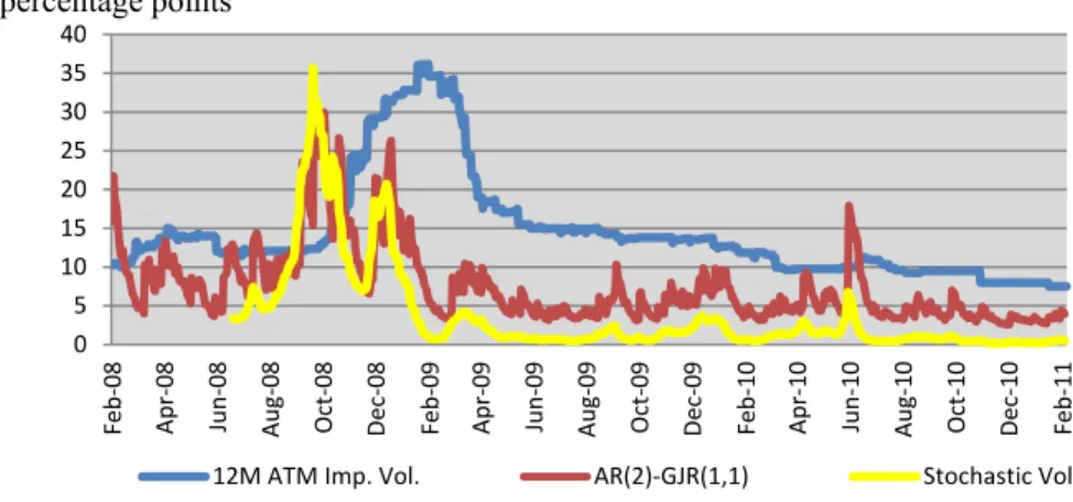
Figure 3.Evolution of conditional, stochastic and implied volatilities
In fact, the implied volatility represents the forecast of conditional volatility. Taking into account the shapes of estimated realized volatility shown in Figure 3, perhaps the predicted volatility would likely be a one step push before of the realized volatility. Looking at the above plot, we can observe that, almost every time, the implied volatility is situated above the realized one, with the exception of the period after Lehman Brothers crash. The trading practices in derivative markets states that if the implied volatility is above forecasted historical one, professional investors should enter on short position on EUR/RON, except the case when in the local exchange rate market is a lot of uncertainty regarding the future evolution of domestic currency. The main key insight of this analysis is the shock felt after the starting of current financial crisis posted permanent effects on implied volatility.
Therefore, in the second timeframe we come to analyse the link between implied volatility and the evolution of EUR/RON rate. We treat this problem econometric in two ways, namely through the usage of co-integration and the dynamic correlation between the two series. Using a VECM model, we determined how much the implied volatility and EUR/RON returns co-integrate in an econometric sense.
0 5 10 15 20 25 30 35 40 Feb ‐ 08 Apr ‐ 08 Jun ‐ 08 Aug ‐ 08 Oct ‐ 08 Dec ‐ 08 Feb ‐ 09 Apr ‐ 09 Jun ‐ 09 Aug ‐ 09 Oct ‐ 09 Dec ‐ 09 Feb ‐ 10 Apr ‐ 10 Jun ‐ 10 Aug ‐ 10 Oct ‐ 10 Dec ‐ 10 Feb ‐ 11
12M ATM Imp. Vol. AR(2)‐GJR(1,1) Stochastic Vol.
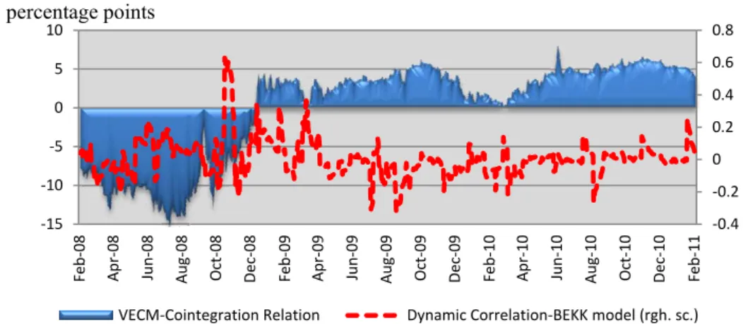
Figure 4.Evolution of cointegration and correlation between 12M ATM implied volatility and EUR/RON evolution
Estimated results showed that cointegrations between the two series became positive definitively after the Lehman episode, which means the EUR/RON returns had to increase in order to achieve the equilibrium. On the other hand, the dynamic correlation between 12M ATM implied volatility and EUR/RON evolution, estimated with BEKK model, fluctuated a lot within the interval + 0.2% and – 0.2%. Exception makes the period between October-December 2008, when the level of correlation ranged within 0.6% – 0.7%.
4. Conclusions
In this paper we intend to identify and analyze, if it is the case, an “epidemiological” relationship between forecasts of professional investors and short-term developments in the EUR / RON exchange rate. We used two different approaches for fitting historical volatility in order to assure robustness for the final results. The first method used to estimate the historical volatility is based on a conditional mixture model of the form AR (2)-GJR (1, 1). The second approach that we called here is based on a stochastic formulation on the volatility of underlined process. From the firs analysis we conclude that, almost every time, the implied volatility is situated above the realized one, with the exception of the period after Lehman Brothers crash. The trading practices in derivative markets states that if the implied volatility is above forecasted historical one, professional investors should enter on short position on EUR/RON, except the case when in the local exchange rate market is a lot of uncertainty regarding the future evolution of domestic currency. The main key
‐0.4 ‐0.2 0 0.2 0.4 0.6 0.8 ‐15 ‐10 ‐5 0 5 10 Feb ‐ 08 Apr ‐ 08 Jun ‐ 08 Aug ‐ 08 Oct ‐ 08 Dec ‐ 08 Feb ‐ 09 Apr ‐ 09 Jun ‐ 09 Aug ‐ 09 Oct ‐ 09 Dec ‐ 09 Feb ‐ 10 Apr ‐ 10 Jun ‐ 10 Aug ‐ 10 Oct ‐ 10 Dec ‐ 10 Feb ‐ 11
VECM‐Cointegration Relation Dynamic Correlation‐BEKK model (rgh. sc.)
insight of this analysis is the shock felt after the starting of current financial crisis posted permanent effects on implied volatility.
Therefore, in the second timeframe we come to analyse the link between implied volatility and the evolution of EUR/RON rate. We treat this problem econometric in two ways, namely through the usage of co-integration and the dynamic correlation between the two series. Using a VECM model, we determined how much the implied volatility and EUR/RON returns co-integrate in an econometric sense. Estimated results showed that cointegrations between the two series became positive definitively after the Lehman episode, which means the EUR/RON returns had to increase in order to achieve the equilibrium. On the other hand, the dynamic correlation between 12M ATM implied volatility and EUR/RON evolution, estimated with BEKK model, fluctuated a lot within the interval + 0.2% and – 0.2%. Exception makes the period between October-December 2008, when the level of correlation ranged within 0.6%-0.7%.
Even the obtained results require further investigation in order to be able to talk about the structural relationship between implied volatility and the evolution of EUR/RON rate, this paper represent a first stage for this type of analysis focused on the Romanian exchange rate market and should be treated accordingly.
Acknowledgements
This work was co-financed from the European Social Fund through Sectoral Operational Programme Human Resources Development 2007-2013; project number POSDRU/107/1.5/S/77213 „Ph.D. for a career in interdisci-plinary economic research at the European standards”.
Notes
(1)
The VEC operator vectorizes a matrix by stacking its columns.
The Kronecker product of two matrices, A and B, where A is m x n and B is p x q is defined
as: ⊗
⋱
which is an mp x nq matrix. There is an
important relationship between the Kronecker product and the VEC operator:
⨂
(2)
For two matrices of the same dimensions, , ∈ the Hadamard product ∙ is a
matrix of the same ⨀ ∈ with elements given by ⨀ , , , . Note
(3)
If a linear combination of I (1) series is stationary, i.e. I (0), the series are called cointegrated. If there are 2 processes and are both I(1) and , with
trend-stationary or simply I(0), then and are called cointegrated.
(4)
Here the term local denotes that our analysis is concentrated only on the transactions rulled out on Romanian exchange market.
(5)
For example, the obtianed conditional volatility with a model from the ARCH class it is sensitive to the conditional mean.
References
Alupoaiei, A., Codîrlaşu, A., Săndică, A.M. “Analysing movements in investor’s risk aversion using the Heston volatility model” (forthcoming)
Alupoaiei, A. (2010). “Analyzing Asymmetric Dependence in Exchange Rates using CopulaS”, Journal Advances in Economic and Financial Research - DOFIN WP Series, No. 44 Andersen, L., Andreasen, J. (2000). “Jump-Diffusion Processes: Volatility Smile Fitting and
Numerical Methods for Option Pricing”, Review of Derivatives Research, 4, pp. 231-262 Andersen, L. (2008). Simple and efficient simulation of the Heston stochastic volatility model,
The Journal of Computational Finance, 11(3), 1-42
Bakshi, G., Cao, C., Chen, Z. (1997). “Empirical Performance of Alternative Option Pricing Models”, Journal of Finance, 52, pp. 2003-2049
Bates, D. (1996). “Jumps and Stochastic Volatility: Exchange Rate Processes Implicit in Deutsche Mark Options”, Review of Financial Studies, 9, pp. 69-107
Carr, P., Madan, D. (1999). “Option valuation using the fast Fourier transform”, Journal of Computational Finance, 2, pp. 61-73
Derman, E., Kani, I. (1994). “Riding on a Smile”, RISK, 7(2), pp. 32-39
Drăgulescu, A.A., Yakovenko, V.M. (2002). “Probability distribution of returns in the Heston model with stochastic volatility”, Quantitative Finance, 2, pp. 443-453
Dupire, B. (1994). “Pricing with a Smile”, RISK 7(1), 18-20
Fengler, M. (2005). Semiparametric Modelling of Implied Volatility, Springer, Berlin
Fouque, J.-P., Papanicolaou, G., Sircar, K.R. (2000). Derivatives in Financial Markets with Stochastic Volatility, Cambridge University Press, Cambridge
Garman, M.B., Kohlhagen, S.W. (1983). “Foreign currency option values”, Journal of International Money & Finance, 2, pp. 231-237
Gatheral, J. (2006). The Volatility Surface: A Practitioner’s Guide, Wiley, New Jersey
Glasserman, P. (2004). Monte Carlo Methods in Financial Engineering, Springer-Verlag, New York
Hakala, J., Wystup, U. (2002). Heston’s Stochastic Volatility Model Applied to Foreign Exchange Options, inJ. Hakala, U.Wystup (eds.) Foreign Exchange Risk, Risk Books, London
Heston, S. (1993). “A Closed-Form Solution for Options with Stochastic Volatility with Applications to Bond and Currency Options”, Review of Financial Studies, 6, pp. 327-343 Hull, J., White, A. (1987). “The Pricing of Options with Stochastic Volatilities”, Journal of
Finance, 42, pp. 281-300
Lee, R., (2004). “Option pricing by transform methods: extensions, unification and error control”, Journal of Computational Finance, 7(3), pp. 51-86
Merton, R. (1973). “The Theory of Rational Option Pricing”, Bell Journal of Economics and Management Science, 4, pp. 141-183
Merton, R. (1976). “Option Pricing when Underlying Stock Returns are Discontinuous”, Journal of Financial Economics, 3, pp. 125-144
Rubinstein, M. (1994). “Implied Binomial Trees”, Journal of Finance, 49, pp. 771-818
Stein, E., Stein, J. (1991). “Stock Price Distributions with Stochastic Volatility: An Analytic Approach”, Review of Financial Studies, 4(4), pp. 727-752
Weron, R. (2004). Computationally intensive Value at Risk calculations, in: Handbook of Computational Statistics, J.E. Gentle, W. Hardle and Y. Mori, Springer, Berlin
Weron, R., Wystup, U. (2005). Heston’s model and the smile, inP. Cizek, W. Hardle, R. Weron (eds.) Statistical Tools for Finance and Insurance, Springer, Berlin