Gait and balance kinematic control for a humanoid robot based on dual quaternion algebra

(1)

m

α

cr

φ

@ufmg

Universidade Federal de Minas Gerais

Programa de Pós-Graduação em Engenharia Elétrica

Research group MACRO - Mechatronics, Control and Robotics

GAIT AND BALANCE KINEMATIC CONTROL

FOR A HUMANOID ROBOT BASED ON DUAL

QUATERNION ALGEBRA

Ana Christine de Oliveira Belo Horizonte, Brazil

(2)

Ana Christine de Oliveira

GAIT AND BALANCE KINEMATIC CONTROL

FOR A HUMANOID ROBOT BASED ON DUAL

QUATERNION ALGEBRA

Thesis submitted to the Graduate Program in Electri-cal Engineering of Escola de Engenharia at the Univer-sidade Federal de Minas Gerais, in partial fulﬁllment of the requirements for the degree of Master in Electrical Engineering.

Advisor: Bruno Vilhena Adorno

(3)

(4)

(5)

Acknowledgements

First of all, I would like to thank my beloved parents, José Antônio and Maria Dinazarde, who have supported me unconditionally in this journey. I have a great pride and admiration for them, for their strength, kindness and persistence.

To my brother and best friend of a life, José Antônio Jr., who had encouraged me at the very beginning to enter in the engineering world, for being my biggest reference when it comes to creative engineering and persistence.

To Marcelino Almeida, for stimulating me to always foster the best results in all aspects of my life. He has always been an enthusiastic partner and has supported me in every single moment of this journey.

A special thanks to my advisor, or as he says, my academic father, Prof. Bruno Adorno, for accepting me as his student and guiding me in this extraordinary world of Master studies. He has contributed in all aspects of this work, not only with theoretical and practical advices and remarks, but also with lessons that helped me to improve my professional skills, and I am very grateful for that. He has an admirable argumentation ability, and is capable of pointing out many relevant issues invisible for the most part of people, and he will always be a great source of inspiration in my academic life.

I would like to acknowledge Prof. Patricia Pena and Prof. Ricardo Takahashi, my undergraduate advisors, for sharing valuable lessons and thoughts with me, and for encouraging me to pursue the academic life. In particular to Prof. Patrícia, thanks for being my female reference in this mannish engineering world, and for supporting me in my academic decisions.

To the members of MACRO, and also cohabitants of LCR: Alex, Antônio, Daniel, Diana, Eduardo, Ernesto, Frederico, Fredy, Gabriela, Heitor, Juan, Jaime, Laysa, Leandro, Lucas, Marcelo, Mariana, Priscilla, Rafael, Rigoberto, and Stella. Thanks for cheering up my daily life, and for sharing laughs, reﬂections, and frustrations throughout this time. Special thanks to Ernesto, who patiently and kindly helped me with many theoretical, practical, and sometimes, existential doubts.

I acknowledge Prof. Guilherme Raﬀo and Prof. Leonardo Torres, for accepting to be reviewers of my thesis, and for their keen remarks on the text.

To the PPGEE faculty members, a special acknowledgment, for their educational

(6)

excellence that makes the Graduate Program in Electrical Engineering of UFMG one of the bests of Brazil. Their thorough analysis about engineering issues are a source of inspiration to pursue excellence in our works.

I also would like to thank the PPGEE administrative staﬀ, for providing me the infrastructure that I needed to work, specially to Jerônimo Coelho and Prof. Rodney Saldanha.

“Whether you think you can, or you think you can’t–you’re right.”

Henry Ford

(7)

Resumo

Este trabalho apresenta uma nova metodologia baseada na álgebra de quatérnios duais (QDs) para obter o modelo cinemático de um robô humanóide, e propõe uma estratégia de controle que satisfaz as restrições cinemáticas garantindo uma caminhada estável. O método de modelagem apresentado consiste de três etapas: modelagem dos membros do robô, modelagem do centro de massa e modelagem do comportamento cooperativo das pernas, utilizando o Espaço de Cooperação Dual. As vantagens deste novo método de modelagem são a sua compacidade e menor esforço computacional demandado para calcular o modelo, quando comparado com métodos baseados em matrizes de transformação homogêneas (MTH), uma vez que os QDs têm apenas oito parâmetros, enquanto as MTHs têm doze. Além disso, a multiplicação de QDs é mais barata computacionalmente que a multiplicação de MTHs e os seus coeficientes podem ser diretamente utilizados na lei de controle, ao contrário das MTHs. A estratégia de controle foi projetada utilizando a pseudoinversa da matriz Jacobiana, a qual representa a tarefa da caminhada, com um termo defeed-forward, e uma tarefa adicional, projetada para manter os braços próximos de uma configuração desejada, foi incluída no espaço nulo desta matriz Jacobiana. O modelo obtido, bem como o controlador proposto, foram validados utilizando o software de simulação de realidade virtual para sistemas robóticos V-REP. Foi verificado que os dados estimados utilizando o modelo e os valores calculados pelo simulador (considerados como dados medidos) se aproximaram bastante, evidenciando que o método de modelagem fornece informações confiáveis. Além disso, o robô controlado pela estratégia proposta foi capaz de executar diferentes movimentos de caminhada com sucesso, além de ser capaz de manter o equilíbrio até mesmo quando os braços estavam se movendo. Este trabalho é a primeira etapa do Projeto Popeye, cujo objetivo geral é construir uma plataforma de testes para um robô humanóide real.

(8)

(9)

Abstract

In this work, we present a novel method to obtain the kinematic model for a humanoid robot based on dual quaternion (DQ) algebra, and propose a control strategy that fulﬁlls the kinematic constraints for a balanced gait. The modeling method consists of three stages: the robot’s limbs modeling, the center of mass modeling, and the legs cooperative behavior modeling using the Cooperative Dual Task-Space Framework. The advantages of the novel modeling method are its compactness and lower computational eﬀort required to calculate the model, when compared with methods based on homogeneous transformation matrices (HTMs), since DQs has only eight parameters whereas HTMs has twelve. In addition,

DQs multiplications are less expensive than HTMs multiplications and its coefficients can be directly used in a control law, differently from HTMs. The presented control strategy was designed using the pseudo-inverse of a Jacobian matrix representing the locomotion task with a velocity feed-forward term, and an additional task, designed to keep the arms close to the desired configuration, was included in the null space of this Jacobian matrix. We validated the obtained model and the proposed controller using the virtual reality simulation software for robotic systems V-REP. The data estimated using the model and the one calculated by the simulation software (which we consider as the measured values) were very close, showing that the modeling method provides reliable information. Furthermore, the robot successfully performed different walking motions when controlled by the proposed strategy, and was capable of keeping the balance even when the arms were moving. This work is the first stage of the Popeye Project, whose goal is to build a test framework for a real humanoid robot.

(10)

(11)

List of Figures

1.1 Recently developed humanoid robots. . . 4

1.2 Poppy robot. . . 5

2.1 3DLIMP related to a humanoid robot. . . 11

3.1 Example of the projection of a point. . . 22

3.2 Example of a rigid motion represented by the dual quaternion in Example (3.2). 24 3.3 Cooperative variables. . . 29

4.1 Robot’s limbs frames and coordinate transformations. . . 33

4.2 Estimated CoM of robot’s links. . . 35

4.3 Joints inﬂuence in the CoM cb 14. . . 37

4.4 Cooperative variables of the robot’s legs. . . 38

5.1 Support polygon of a humanoid robot. . . 41

5.2 Cart-table model. . . 43

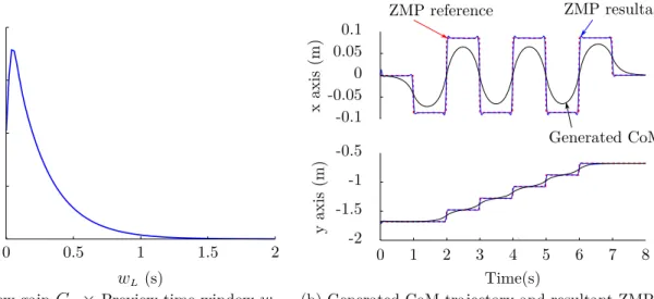
5.3 Results of the walking pattern generation method. . . 47

5.4 Comparison of the ZMP Resultant for diﬀerent values of Qx. . . 47

5.5 Example of a cubic Bézier curve. . . 48

5.6 Pulse function example. . . 49

5.7 Trajectory generated by (5.11). . . 50

5.8 Complete position trajectories of the feet generated by (5.12). . . 51

5.9 Linear velocities of the feet generated by (5.13). . . 51

5.10 Circular Path of Example (5.4). . . 54

6.1 Structure of the simulation framework. . . 63

6.2 Humanoid robot ASTI. . . 63

6.3 DH convention for ASTI. . . 64

6.4 Robot conﬁguration during the validation. . . 65

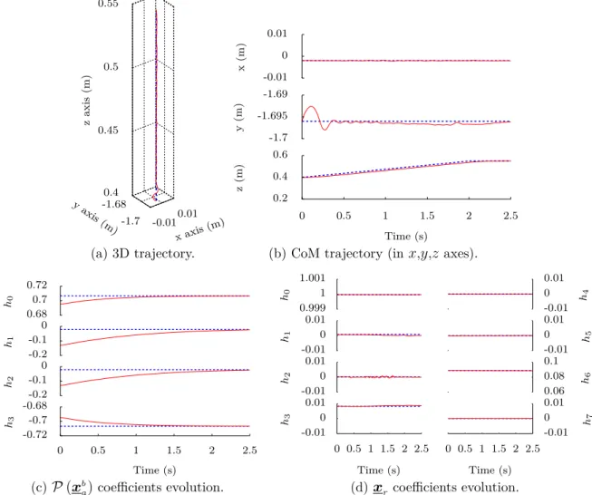
6.5 CoM and CoM linear velocity validation. . . 66

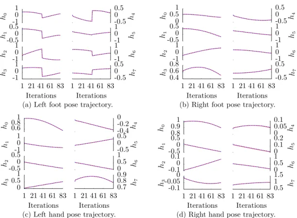
6.6 Poses of the limbs end-eﬀectors during validation. . . 66 6.7 Linear and angular velocities of the limbs end-eﬀectors during validation. 67

(14)

6.8 Results obtained from the execution of a circular trajectory. . . 69 6.9 Results obtained from the execution of the standing up movement.. . . 70 6.10 Simulation snapshots of the standing up movement. . . 71 6.11 Results obtained from the execution of the second pattern controlled using

the strategy 1. . . 72 6.12 Feet trajectories obtained from the execution of the second pattern controlled

using the strategy 1. . . 73 6.13 Simulation snapshots from the execution of the second pattern controlled

using the strategy 1. . . 74 6.14 Comparison of the results obtained from the execution of the ﬁrst pattern

controlled using strategies 1 and 2. . . 75 6.15 Results obtained from the execution of a walking motion controlled using

the strategy 2, where the arms were actuated. . . 77 6.16 Simulation snapshots of a walking motion controlled by the strategy 2, while

moving the arms. . . 78 6.17 Angles of the arms joints during the walking motion controlled using the

strategy 3, where the arms were actuated. . . 79 6.18 Results obtained from the execution of a walking motion of 50 footsteps,

controlled using the strategy 3, which includes the arms in the control law. 80 6.19 Simulation snapshots of a walking motion of 50 footsteps, controlled using

the strategy 3, which includes the arms in the control law. . . 81 6.20 Arms joints angles during a walking motion of 50 footsteps, controlled using

the strategy 3, which includes the arms in the control law. . . 82 6.21 Results obtained from the execution of a walking motion of 50 footsteps,

controlled using the strategy 4. . . 83 6.22 Angles of the arms’ joints during a walking motion of 50 footsteps, controlled

using the strategy 4. . . 84 6.23 Results obtained from the execution of a walking motion controlled using

the strategy 4, where the arms were actuated. . . 84 6.24 Angles of the arms joints during the walking motion controlled using the

strategy 4. . . 85 6.25 Simulation snapshots of a walking motion controlled by the strategy 4, while

moving arms. . . 86 6.26 Results obtained from the execution of a walking motion in a semi-circle

shaped path, controlled using the strategy 4. . . 87 6.27 Footprints executed in a walking motion in a semi-circle shaped path,

controlled using the strategy 4. . . 88

A.1 Right arm scheme. . . 101

(15)

A.3 Left and right leg scheme. . . 102

B.1 Results obtained from the execution of a trajectory deﬁned by a sine in the xy plane. . . 103 B.2 Results obtained from the execution of a trajectory deﬁned by a sine in the

xz plane. . . 104 B.3 Comparison of the results obtained from the execution of the second pattern

controlled using strategies 1 and 2. . . 105 B.4 Comparison of the results obtained from the execution of the third pattern

controlled using strategies 1 and 2. . . 106 B.5 Comparison of the results obtained from the execution of the forth pattern

controlled using strategies 1 and 2. . . 107 B.6 Comparison of the results obtained from the execution of the ﬁrst pattern

controlled using strategies 2 and 4. . . 108 B.7 Comparison of the results obtained from the execution of the second pattern

controlled using strategies 2 and 4. . . 109 B.8 Comparison of the results obtained from the execution of the third pattern

controlled using strategies 2 and 4. . . 110 B.9 Comparison of the results obtained from the execution of the forth pattern

controlled using strategies 2 and 4. . . 111

(16)

(17)

List of Tables

6.1 Robot’s links masses. . . 64

6.2 Summary of the proposed control strategies. . . 72

6.3 Index comparison between strategies 1 and 2. . . 76

6.4 Control Strategy 4 comparison indexes. . . 82

A.1 DH Parameters of right arm. . . 101

A.2 DH Parameters of left arm. . . 101

A.3 DH Parameters of left and right legs. . . 102

(18)

(19)

Acronyms

3D Three-Dimensional

3DLIPM Three-Dimensional Linear Inverted Pendulum Mode

3MLIMP Three-Mass Linear Inverted Pendulum Mode

AIST National Institute of Advanced Industrial Science and Technology

API Application Programming Interface

ASIMO Advanced Step in Innovative Mobility

BIPMAN Bipedal Walking Machine

CDTS Cooperative Dual Task Space

CoM Center of Mass

DFKM Diﬀerential Forward Kinematics Model

DH Denavit-Hartenberg

DOF Degrees of Freedom

DQ Dual quaternion

DSP Double-Support Phase

FKM Forward Kinematics Model

GCIPM Gravity-Compensated Inverted Pendulum Mode

GCoM Center of Mass Projection on the Ground

HRP Humanoid Robotics Project

HTM Homogeneous Transformation Matrix

IK Inverse Kinematics

(20)

IAVU Integrated Absolute Variation of the Control signal

MACRO Mechatronics, Control, and Robotics

MAE Mean Absolute Error

PID Proportional Integral Derivative

ROS Robot Operating System

SESC Statically Equivalent Serial Chain

SSP Single-Support Phase

SVD Singular Value Decomposition

UFMG Universidade Federal de Minas Gerais

WL-3 WASEDA LEG-3

WL-10R WASEDA LEG-10 REFINED

WL-12 WASEDA LEG-12

ZMP Zero Moment Point

(21)

Notation

Γ Function representing the trajectory of one foot.

ε Dual unit.

λ Scalar gain of the control law.

µ Step function.

φ Rotation angle.

Π∆t Pulse function with time duration of ∆t.

Ψx,Ψy Performance indexes of the preview control method.

Bn

i Bernstein polynomial of order n.

C8, C4 Conjugating matrices.

dh Step height.

d Dual number.

D Operator to extract the dual part of dual quaternions.

e Error between the reference and actual values in the control law.

F Coordinate system or frame.

H Set of dual quaternions.

H Set of quaternions.

+

H4,H−4 Hamilton operators. +

H,H− Hamilton operators extended for dual quaternions. I Identity matrix.

is Step index.

(22)

ˆı,,ˆˆk Quaternion (or imaginary) units.

L, M, N, X Matrices or vectors.

Ns Number of steps.

J Jacobian matrix.

J+ _{Pseudo-inverse of the Jacobian matrix.}

ˆ

J Extended Jacobian matrix.

¯

J Jacobian matrix obtained by removing the last row of J (associated with

z-axis).

JA _{Jacobian matrix with respect to frame}

FA.

JP, JD Jacobian matrices related with the primary and dual parts of J.

Jori, Jpos Orientation and position Jacobian matrices.

Jr, Ja Cooperative Jacobian matrices (relative and absolute).

n Pure quaternion representing the rotation axis.

P Operator to extract the primary part of dual quaternions.

pA

AB Quaternion representing the translation from the frameFA to FB with respect

toFA.

pA _{Quaternion representing a point with respect to a frame} _F A.

q Joints vector.

rA

B Unit quaternion representing a rotation from frameFA toFB (moving frames

notation).

T Sampling time.

h,x,y Quaternions.

h,x,y Dual quaternions.

x∗ _{Dual quaternion conjugate.}

x{λ} _{Dual quaternion exponentiation.}

kx_k Dual quaternion norm.

xB

A Complete pose of a frameFA with respect to FB.

(23)

vec4,vec8 Vec operators representing a one-to-one mapping from H _to R4 _or _H _to _R8_, respectively.

wL Preview time window.

(24)

1

Introduction

Biped robots are a particular case of legged robots, whose locomotion is achieved by the coordination between two legs. They are more versatile when compared with conventional wheeled robots, since they have higher mobility in human environments thanks to its pecu-liar characteristic of discontinuous contact with the ground, which allows the locomotion in rough terrains, stairs climbing, and obstacles avoidance. However, biped robots tends to easily tip over in real environments. Therefore, it is necessary to develop a controller that meets all constraints required for a balanced walk.

Humanoid robots, or simply humanoids, are a class of biped robots whose body shape resembles the human body, i.e. with two arms, two legs, one torso, and one head. This type of robots arouses interest on the scientiﬁc community since the 1970s, mainly due its similarity with the human body, which makes it easier to interact with human tools and environments, such as door pullers, stairs, automobiles, valves, etc. Humanoids can be used to access and handle tools in harmful and dangerous zones, like in the case of nuclear accidents or buildings with compromised structures (Siciliano & Khatib, 2008).

A curious fact about this type of robots comes from a work published by Mori et al. (2012), where they deﬁne the “uncanny valley.” This work shows how human beings

react in the presence of human-like entities, and one conclusion is that human beings are familiar with humanoid robots almost as they are with themselves. Thus, another interesting application of humanoids is in assistive tasks, as carring and supporting elderly or physically disabled people, or in treatments of psychological disorders such as autism. According to Fukuda et al. (2012), robots locomotion can be classiﬁed into two

(25)

categories: quasi-static and dynamic locomotion. As defined by Mason (1985, apud Siciliano et al. 2008), in quasi-static robot systems, the effects generated by accelerations and inertial forces are negligible, and, in this case, the system is modeled as a transition between discrete configurations. Furthermore, in this case, it is assumed that the robot is statically stable, i.e. if the locomotion is interrupted the robot keeps a stable posture. The first approach can be used to achieve slow walking-speeds, and it is possible to be performed only on flat surfaces. The second approach allows a better performance, achieving faster walking-speeds, including running, and a flat surface is not required in this case. Thus walking on uneven or rough terrains, as well as stairs climbing, is only possible assuming a dynamic locomotion.

The autonomous locomotion of humanoids is a very challenging subject, and depending on the desired behavior and application, the dynamic or the kinematic approach can be adopted in its modeling and control. This class of robots has a large number of Degrees of Freedom (DOF), and obtaining a dynamic model in this case requires extensive calculations. Furthermore, the dynamic model of this kind of structure can eventually change when interacting with the environment, and the controller must be designed to be robust or adapt to these situations. On the other hand, the kinematic modeling does not suﬀer from these problems, however, this approach has a limitation regarding the locomotion velocity and the environment structure, since it does not allow fast locomotion and walking on rough terrains. Moreover, in this case, the model does not take into consideration the forces related to the movement.

This work focuses on the kinematic approach to model and control a humanoid robot, and we adopt a representation based on dual quaternion (DQ) algebra. The most commonly used representation within the context of kinematics, robotics, and control systems are the homogeneous transformation matrices (HTMs), since they are a singularity-free representation and can be used to express rigid motions. However, in the last two decades, DQs have gained popularity in this context, because they also represent rigid motions without suﬀering from representational singularities, and are more compact than HTMs, since the former have only eight parameters whereas the latter have twelve. Moreover, DQ multiplications are less expensive than HTMs multiplications, and its coeﬃcients can be directly used in a control law, which, to the best of our knowledge, has not been done in the case of HTMs (Adorno, 2011).

(26)

1.1. HISTORICAL BACKGROUND 3

1.1 Historical Background

The ﬁrst known record about humanoid robots was found in Leonardo Da Vinci’s notebook, possibly conceived around 1495 and rediscovered in the 1950s by Carlos Pedretti, a professor of the University of California (Rosheim, 2006). The designed mechanism—called “Robot Knight”—was composed of a series of pulleys and cables, and could stand, sit, raise its visor, and maneuver its arms, independently.

The first biped robots with actuated joints were developed by Ichiro Kato and his colleagues from the Department of Mechanical Engineering of the School of Science and Engineering of the University of Waseda in Tokyo. In 1968, they built the lower-limbs mechanical model WASEDA LEG-3 (WL-3), which was electro-hydraulic actuated and was capable to perform a human-like gait, stand and sit. One year later, they designed a biped robot with an anthropomorphic appearance that was pneumatically activated, called WAP-1. The first human-body sized robot was built in 1973, named WABOT-1, which had a limb-control system, an image processing unit and an embedded speech and interaction system. In addition to walking locomotion, this robot was able to carry and manipulate objects with its hands.

The robot WASEDA LEG-10 REFINED (WL-10R) was presented in 1982 by A. Takanishi, who was a collaborator of Ichiro Kato, and his colleagues. It represented a landmark in humanoid robots history as the first robot to execute dynamic locomotion. In 1984, some researchers from the University of Tokyo developed the BIPER Series, which were all statically unstable, but could execute dynamic locomotion. BIPER 1 and 2 were capable to walk only in the sideway direction whereas BIPER 3 could also walk in forward and backward directions. BIPER 3 has only a point contact between the leg and the ground; thus, to stay upright, the robot must keep executing successive steps, continuously.

R. Katoh and M. Mori built in 1984 the BIPMAN (Bipedal Walking Machine) robot, which was a new paradigm in the context of biped robots, since it was constituted by two telescopic legs without knees that could extend and contract to perform the locomotion. In 1985, Jessica Hodgins and Marc Raibert developed a biped robot hydraulically actuated that was able to jump up to 67 cm and run with a speed up to 4 m/s.

Ishiro Kato and his coworkers once again presented an innovation in 1986 with the robot WASEDA LEG-12 (WL-12), which was the first to perform dynamic walking with trunk compensation. In 1990, Tad McGeer developed the first 1 DOF biped robot with articulated legs and no actuation, capable to perform locomotion in a downhill slope, so called “passive walking,” generated by the interaction between gravity and inertia.

(27)

also recognize faces and map environments. It is one of the most complete humanoid robot available in the market. Along with ASIMO, some recently presented humanoids are the NAO by AldebaranT M_{, the Atlas by Boston Dynamics}T M_{, and the HRP (Humanoid}

Robotics Project) series developed by the National Institute of Advanced Industrial Science and Technology (AIST), like the HRP-4C. These robots are all depicted in Figure 1.1.

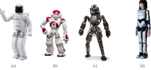
(a) (b) (c) (d)

Figure 1.1: Recently developed humanoid robots. From left to right: (1.1a) ASIMO robot1_, (1.1b) NAO robot2_, _{(1.1c) Atlas robot}3_, _{and (1.1d) HRP-4C robot}4_.

For a more comprehensive survey on the humanoid robots history, see André et al. (2004).

1.2 Objectives

This work was developed within the research group MACRO (Mechatronics, Control, and Robotics) and is part of the Popeye Project, whose main goal is to build at UFMG a humanoid robot for the study of whole-body control techniques and human-robot interaction. This humanoid robot, which is depicted in Figure 1.2, is a result of an initiative of the INRIA Institute, called Poppy Project. It consists of an open-source platform for the creation and assembly of the robot’s 3D printed parts, and oﬀers libraries to control the robot’s joints and behavior.

The work herein presented is a conceptual part in the development of Popeye Project, focusing on the locomotion, which is a fundamental part to implement a testbed for the humanoid robot. Its objectives are listed below:

(28)

1.3. CONTRIBUTIONS 5

Figure 1.2: Poppy robot5_.

1. Development of a kinematic model for the whole-body and Center of Mass, for a generic humanoid robot;

2. Development of a gait and balance controller for the robot, based on the work of Park & Lee (2013); Adorno et al. (2010), using the DQ algebra and the Cooperative Dual Task-Space Framework.

1.3 Contributions

Within the scope of UFMG, the contribution of this work relies on the replication and vali-dation of the results found in the literature, using a virtual reality simulation environment. This is an important stage for a better understanding of the consolidated works about humanoid robots, which is fundamental to build a reliable testbed for a humanoid robot.

The scientiﬁc contribution of this work consists in the adoption of the DQ algebra in the humanoid’s kinematic model conception, since it was not found in the related literature. Moreover, we proposed enhancements in the original control strategy by Park & Lee (2013) so as to reduce the control eﬀort and also to allow wide range arms movements during the walking motion, still keeping the robot balanced.

Some partial results of this work were published in the XII SBAI - Simpósio Brasileiro de Automação Inteligente (in English: Brazilian Symposium of Intelligent Automation) (Oliveira & Adorno, 2015).

(29)

1.4 Structure of the Text

This thesis is organized into seven chapters, summarized as follows:

Chapter 2 presents some of the most important works on humanoid robots, compre-hending modeling methods, walking pattern generators, and gait controllers.

Chapter 3 reviews the mathematical background needed to understand the presented methods and establishes the notation used throughout this dissertation.

Chapter 4 describes the methodology to obtain the humanoid’s kinematic model using DQ algebra.

Chapter 5 summarizes the stability conditions for a balanced locomotion, and details the methods to obtain the reference trajectories for the control. Furthermore, the control strategy adopted is presented and some improvements on the techniques present in the literature are proposed.

In Chapter 6, the experimental platforms are presented, the performed trials are described, and the corresponding results are analyzed.

Chapter 7 presents an overview of the entire work and some steps and improvements for future works are proposed.

(30)

2

State of the Art

This chapter discusses the related works recently developed within the biped robots ﬁeld, and is organized as follows: Section 2.1 highlights the existing modeling methods and conventions applied speciﬁcally to biped robots; Section 2.2 presents the most consolidated walking pattern generation methods; and Section 2.3 discusses some control strategies for gait and balance of biped robots .

2.1 Modeling of Biped and Humanoid Robots

The Denavit-Hartenberg (DH) convention (Hartenberg & Denavit, 1955) is widely adopted in robots kinematic modeling. This convention is used to define frames to each joint, such that the geometric parameters of a robot can be easily used to obtain the robot’s Forward Kinematics Model (FKM). The coordinate transformation between the frames of two consecutive joints is represented by a product of four basic transformations, using the DH parameters (see Section 3.3.1). This convention is frequently adopted to obtain the FKM of biped robots’ limbs (Kofinas et al., 2014; Ali et al., 2010; Chevallereau et al., 2010; Zannatha & Limon, 2009), and is also used in the work herein described. Toscano et al. (2014) propose a different methodology based on the Screw Theory to obtain the robot’s limbs FKMs, by using the concept called “screw displacements” (a rigid motion can be regarded as a combination of a rotation around an axis and a translation along the same axis) to define the relations between the joints of the kinematic chain. This is a methodology concurrent to the DQ algebra, used herein. Since our research group focuses

(31)

on DQ algebra, the adoption of a concurrent methodology becomes inconvenient, because it makes diﬃcult to integrate this work with the rest of the ones developed within the group. Furthermore, the DQ representation, as used in our research group, seems more appropriate for integration with low level kinematic controllers.

According to Sentis (2007), a humanoid robot can be regarded as a free-floating system which has a specified number of joints and a base frame describing its position and orientation. He suggests a virtual spherical joint in series with three virtual prismatic joints to represent the robot’s kinematics, and treats the robot as a holonomic system with n actuated joints and six passive DOFs, where ground reaction forces appear at the contact points with the floor. Chevallereau et al. (2010) extend this interpretation and present two methodologies to obtain the generalized coordinates of the robot: the “Kinematically Free Mode,” which also considers the robot as a free-floating system with the base at the hip center, and the “Rooted Kinematic Chain” mode, which considers the existence of a link in contact with the ground where the system’s base is located, which stays stationary during the whole step-motion. In both approaches, some dynamic constraints are associated with the kinematic model, which specify the conditions for a stable locomotion. The first approach is not interesting in the particular case of this work, since it allows the supporting-foot to move during the step motion whereas it is desired to keep it stationary when it comes to define the system’s reference frame.

In the majority of cases, the robot is controlled in the task space, and the joints configuration must be determined from a desired pose of the robot’s end-effectors. This is the inverse of the FKM, and is known as the Inverse Kinematics (IK) problem. Within the context of biped robots, this problem is usually solved by analytical (Zannatha & Limon, 2009; Tolani et al., 2000; Ali et al., 2010; Kofinas et al., 2014) or numerical (Tevatia & Schaal, 2000) means. In analytical methods, the IK is solved by geometry, relating the robot’s generalized coordinates with its geometric features. For instance, Kofinas et al. (2014) solves the IK problem for a specific robot, while Ali et al. (2010) find a closed-form

that can be used for humanoids with a speciﬁc structure, and they take advantage of this structure in order to simplify the geometry. This method is interesting to determine the IK of speciﬁc robots, and since this work has the objective of determining a general solution, it is not applicable in our case. On the other hand, numerical methods use the system’s Jacobianmatrix—which relates velocities at the robot’s end-effectors with the joints velocities—to obtain the solution of the IK problem. Tevatia & Schaal (2000), for example, use the pseudo-inverse of the Jacobian matrix together with the desired velocities of the end-effectors, to obtain the solution. Another approach is called “Control-theory based”, which consists of casting the differential kinematic model of the system into a control problem, that is solved also using the pseudo-inverse of the Jacobian matrix. This method is addressed by Sciavicco et al. (2000), and is used in Mansard et al. (2009).

(32)

2.1. MODELING OF BIPED AND HUMANOID ROBOTS 9

it is related with the robot’s balance. Plenty of works propose modeling methods relating the robot’s CoM with respect to its joints conﬁguration (Choi et al., 2007; Cotton et al., 2009; Boulic et al., 1995; Phillips & Badler, 1991). The method proposed by Choi et al. (2007) consists in building an equivalent FKM for the robot’s CoM, and its expression

is defined as a weighted sum of the FKMs of the CoM of each link. To obtain the FKM of each link CoM, it is regarded as the end-effector of the corresponding limb, and the links after this one are not considered. In order to solve the IK of the robot’s CoM, a Jacobian matrix is defined by taking the first time derivative, with respect to the joints vector, of the expression representing the FKM. Boulic et al. (1995) and Cotton et al. (2009) use equivalent chains to represent the robot’s CoM. Boulic et al. (1995) propose

the "Augmented Body" associated with a joint, which consists of a rigid body dynamically equivalent to the union of all bodies supported by the joint, for the current state of the system. Likewise, Cotton et al. (2009), defined a concept named “Statically Equivalent Serial Chain (SESC),” which consists of an equivalent chain whose origin is placed at the link in contact with the ground, and whose extremity is coincident with the CoM. It is a one-to-one mapping between the original chain’s joints and the equivalent chain’s joints. The aim of that work is to build a CoM Jacobian matrix for a biped robot without its dynamic parameters, which is used to solve the IK problem for the robot’s CoM. To do that, the configuration of the joints for some stable postures of the robot are recorded and used in a system of linear equations to obtain the parameters of the CoM Jacobian. These methods are very useful when one foot must be stationary on the ground, but they become inconvenient for robot’s in locomotion, when the rooted link changes periodically. Phillips & Badler (1991) use a different approach, where they define the lower part of the robot’s torso as the estimated CoM of the robot, and constraint variables associated with the ankle, the knee, and the hip joints of the rooted leg are defined. If the CoM approximation is different from the expected, the constraints must be solved again to guarantee a balanced posture. This approach gives a good approximation of the robot’s CoM in the case of robots with well-distributed masses among their limbs. However, if the legs are heavier than the upper-body, which frequently happens, the method becomes inefficient, since it will give a poor approximation of the CoM, and, consequently, increasing the computational effort to satisfy the constraints and adjust the posture.

In this work, we adopt the Rooted Kinematic Chain interpretation to build the whole-body kinematic model of the biped robot, using the DH convention to deﬁne the frames of the robot’s joints. The IK problem is solved using the Control-theory based method aforementioned. Finally, to obtain the CoM kinematic model we adopt a methodology similar to the used by Choi et al. (2007), i.e. to build an equivalent FKM for the robot’s CoM, deﬁned as a weighted sum of the FKMs of the CoM of each link.

(33)

dissertation, all transformations are represented by dual quaternions. In the context of biped robots, this approach was only found in Park & Lee (2013), which is focused in the control strategy for the locomotion task, and is better detailed in Section 2.3.

2.2 Walking Pattern

The gait of biped robots is one of the most challenging and exciting ﬁelds in robotics. The walking motion is inherently an unstable movement, thus, in order to keep the robot balanced, some kinematic and dynamic constraints must be fulﬁlled during the motion. The gait is a sequence of coordinate and periodic movements, and its complete cycle is composed of two phases:

• Single-support phase (SSP), when one foot is stationary on the ground, while the other foot is swinging towards the next footprint;

• Double-support phase (DSP), when both feet are in contact with the ground.

In the last decades, some methods were proposed to generate the feet trajectories and the hip trajectory for the gait cycle which fulﬁlls the balance constraints, commonly denoted as “walking pattern.” As long as these trajectories are known, the joints conﬁgurations to execute the walking motion can be determined.

The Zero Moment Point (ZMP) was introduced by Vukobratović et al. (1970) and is deﬁned as a point where the moments around the x-axis and the y-axis generated by reaction forces and reaction torques are zero. It is a commonly used parameter when it comes to analyze the stability of the robot in dynamic locomotion. The Three-Dimensional Linear Inverted Pendulum Mode (3DLIPM) and its variations are widely used in the literature to generate walking patterns for biped robots in ﬂat terrains (Kajita et al., 2001; Tang & Er, 2008; Feng, 2008), and consists in a dynamic model that relates the robot’s ZMP to its CoM. To summarize, the dynamic behavior of the robot during the SSP is approximated by the dynamics of an inverted pendulum, consisting of a telescopic rod with a point mass whose motion is constrained by a plane. The base of the inverted pendulum is located at the ZMP, and the point mass represents the robot’s global CoM. The 3DLIPM related to a humanoid robot is illustrated in Figure 2.1.

The ZMP is assumed to be close to the foot center, and the ZMP trajectory is deﬁned by the desired footprints, which are determined by a periodic function regarding the desired walking speed, and the time duration of the SSP and the DSP. Thus, the CoM trajectory is determined from the ZMP trajectory using the dynamic equations of the system.

(34)

2.2. WALKING PATTERN 11

ZMP CoM

Figure 2.1: 3DLIMP related to a humanoid robot.

according to the terrain conditions. Consequently, the ZMP trajectory is not defined by a known function, and the aforementioned method using the 3DLIPM is not appropriate to obtain the CoM trajectory. Aiming to solve this issue, Kajita et al. (2003) and Kim (2007) proposed methods to determine the CoM trajectory from arbitrary trajectories of the ZMP, also based on 3DLIPM. Kajita et al. (2003) proposed a method based on preview control1_, where the current input of the system, which is the current CoM reference, is calculated using future references of the known ZMP trajectory. They presented a discrete state space system that models the dynamics of the 3DLIPM, and used the associated matrices to calculate the preview control gains, and to determine the CoM reference. Kim (2007), on the other hand, proposed a convolution sum method to find the solution, where the 3DLIPM is written in the frequency domain. Its impulse response is determined, which is non-causal, but stable, and the current CoM reference can be calculated through a discrete convolution between the ZMP trajectory and the system’s impulse response, within a finite time window. The convolution result consists of two terms: the first one represents the CoM computed from past information about the ZMP trajectory, and the second term represents the CoM computed from future information about the ZMP trajectory. Adding these two terms, the result is the current CoM reference.

The method proposed by Kajita et al. (2003) is widely used in the context of walking pattern generation for biped robots on account of its eﬃciency and ﬂexibility. However, the robot’s global CoM jerk can reach large values in the presence of disturbances, compromising the robot’s stability. With the objective of solving this issue, Wieber (2006)

1_{Preview control is one of the precursors theories of the predictive control theory, and this is the the}

(35)

proposed an extension of this method, including some constraints in the minimization of the performance index, which is calculated as part of the preview control method. These constraints determine a limit for the CoM jerk and a safe region inside the support polygon where the ZMP is allowed to stay. The drawback of this method is the large computational eﬀort required to solve the constrained optimization problem at each time instant.

Furthermore, Kajita et al. (2003) assumes that the robot’s mass is concentrated at the CoM, and that the free-leg dynamics can be neglected during the SSP. In reality, the leg mass is a large proportion of the robot’s body mass. Consequently, during the SSP, the ZMP moves away from the predefined reference, decreasing the robot’s stability. With the objective of obtaining a more stable controller, Park & Kim (1998) proposed a more accurate model named Gravity-Compensated Inverted Pendulum Mode (GCIPM), which is based on the linear inverted pendulum mode, including the dynamics of the free-leg. The robot is modeled by a two-mass system: one representing the free-leg, located at the swinging-foot, and one representing the rest of the robot’s body, concentrated at the hip. The proposed method assumes a defined trajectory for the swinging-foot, so that the influence of the free-leg mass in the robot’s dynamics can be computed and compensated for by the hip motion.

Another model similar to the 3DLIMP also applied in the literature to generate walking patterns is the Three-Mass Linear Inverted Pendulum Model (3MLIPM) (Galdeano et al., 2013; Feng, 2008). The robot’s dynamics is approximated by the 3MLIPM, which consists in a three-link system with a point mass in each link—one representing the torso, and the two others representing the legs—, being a more accurate model then the single mass linear inverted pendulum model. The method proposed by Feng (2008) is similar to the aforementioned ones, where the footprints are determined for a flat terrain, and the trajectory of the masses is defined according to the dynamic equations of the system. Galdeano et al. (2013) presents an extension of this method, where an optimization of the joints trajectory is made with the objective of minimizing the ZMP movement inside the footprint area to improve the robot’s stability. The contribution of this extension is the possibility of generating walking patterns with direction changes, which is not possible in the work of Feng (2008).

(36)

2.3. CONTROL OF GAIT AND BALANCE 13

support polygon edges, is chosen. Roussel et al. (1998) also presents a method to minimize the energy of the gait cycle, where a dynamic model for each phase of the gait cycle is formulated and a cost function representing the energy injected in the system during the cycle is presented. The aim is to minimize this cost function, given some constraints: the initial and final desired configuration of the robot’s joints in the SSP, the final desired configuration of the robot’s joints in the DSP, the time duration of the SSP, and the time duration of the whole gait cycle. In a non-periodic walking motion, these method becomes inefficient, since the optimization problem must be solved for each step.

In contrast with the presented ideas, Zarrugh & Radcliﬀe (1979) propose a walking pattern generation method in the joints level so that the walking motion mimics the human gait. In order to accomplish that, kinematic data is recorded from a human gait, and the displacements of the joints are determined to formulate the walking pattern. This work gives some interesting insights about the walking motion in the robotics ﬁeld, however it is not very versatile since it does not allow to change the walking directions and to control the locomotion itself.

The choice of the walking pattern generation method is a trade-off between model accuracy and footsteps placement flexibility. In this work, the walking pattern generation method is based on the 3DLIPM, because it is more flexible than others, and allows us to deal with robots whose dynamic parameters are not known, or uncertain. The adopted method is based on the work proposed by Kajita et al. (2003), which is more consolidated in the robotics field, and requires a low computational effort, if compared with the aforementioned works.

2.3 Control of Gait and Balance

Since the feet and CoM reference trajectories are determined by the walking pattern generator, the displacements in the robot’s joints space can be calculated by solving the IK problem. However, the humanoid robot tends to tip over easily in real environments, specially under disturbances. Therefore, the implementation of a balance control is of a particular relevance in locomotion.

(37)

embedded control framework for the CoM, and it allowed the stabilization of the robot’s body on a ground with varying slope. A more complex method is proposed by Hirai et al. (1998), and also presented by Yokoi et al. (2004), by using a set of complementary strategies to formulate the balance controller. One of these strategies—denoted as “Body Inclination Control” or “Ground Reaction Force Control”—consists in modifying the feet position/orientation in order to correct the body’s posture. The other one—denoted as “ZMP Damping Control” or “Model ZMP Control”—attempts to shift the desired ZMP by adjusting the horizontal position of the robot’s torso. Finally, the “Foot Landing Position Control” or “Foot Adjusting Control” has the aim of correcting the relative position of the upper-body and the feet, and can be used to stabilize the robot’s body on uneven terrains, where the feet may be inclined. Li et al. (2012) also developed a controller based on a set of different strategies; however, instead of controlling stiff humanoid systems, the intention is to stabilize compliant robots. The three strategies used are: the “Horizontal Compliance Control,” which is used to make the body’s compliance regulation by using a PID controller based on the ZMP error to modify the robot’s CoM; the “Body Attitude Control” strategy is used to compensate the angular momentum generated by the lower-limbs motion, by rotating the upper-body in the inverse direction; the “Potential Energy Control” stabilizes the robot’s potential energy by constraining the CoM to an inclined plane. The drawback of ZMP based control methods is the need of sensors to measure it, or, in the case of using mathematical relations to estimate it, the large estimation errors.

For static locomotion, a common approach for stabilizing the robot’s posture is to use control strategies based on kinematic-constraints, in which the ZMP information is not taken in consideration, but the CoM projection on the ground (GCoM). Following this idea, some works propose the adjustment of some walking pattern parameters together with the IK to keep the robot balanced during the locomotion (Hof, 2008; Missura & Behnke, 2011; Graf, 2010). Hof (2008) presents a new concept named “Extrapolated Center of Mass (XcoM),” which combines the robot’s CoM projection on the ground and its CoM velocity and simplifies the stability conditions for locomotion. In this method, a feedback controller compensates the foot placements and CoM errors by adjusting the step length or the step time duration. Similarly, Missura & Behnke (2011) propose a control strategy, whose main purpose is lateral disturbance rejection, by adjusting the step time duration and location of the next step after the disturbance, in order to correct the CoM trajectory. With the intention of generating faster gait cycles, Graf (2010) suggested a controller that eliminates the DSP while keeping the robot balanced by adjusting the step time duration. These methods become impractical in cases when the footprints cannot be changed during the walking motion, due to floor constraints for example.

(38)

2.3. CONTROL OF GAIT AND BALANCE 15

GCoM near to the center of the support polygon. The proposed controller uses the pseudo-inverse of the body’s CoM Jacobian matrix to regulate the GCoM on the desired position. Furthermore, the limbs end-effectors poses are controlled to follow the reference in the null space of the robot’s joints configuration, i.e. taking advantage of the robot’s redundancy with respect to the main task, which is the regulation of the GCoM. Hofmann et al. (2009) adopted a strategy based on a Proportional-Derivative controller and the robot’s dynamic model that allows the stabilization of a robot in unstable initial conditions, through the control of the CoM, robot’s orientation, and swing-foot pose, simultaneously . The controller maneuver the robot’s free-leg and torso in order to drive the robot’s body to stable postures. Stephens (2007) combines two strategies to control the biped robot’s posture, with the feet fixed on the ground, in the presence of disturbances: the ankle strategy and the hip strategy. The first one designs a controller which keeps all joints torques neglected, except the ankle joint. As this behavior can lead the global CoM to unstable regions, the hip strategy is applied, which consists of maneuvering the hip angles in order to incline the torso and lead the CoM to the desired target.

Ames et al. (2015) develop a formal controller synthesis for biped robots, consisting of a two-step approach to generate physically realizable stable walking. By formal synthesis we mean that the author works on formal mathematical axioms to obtain the controller. In this work, we do not take into consideration the forces involved in the movement. As stated in Chapter 1, the humanoid robots locomotion can be classified into quasi-static and dynamic locomotion, and in quasi-static locomotion the effects of accelerations and inertial forces are negligible. Thus, we assume a quasi-static locomotion herein, even though a dynamic parameter is compensated in our control method (the robot’s CoM). As a consequence, the ZMP based control methods are not applicable in our work, since they deal with dynamic locomotion, which is not our focus. Moreover, the methods to control the robot’s posture in standing configurations do not address the locomotion control problem. Therefore, they are not appropriate in our case, and were presented just for the sake of information. About the formal method to controller synthesis, although it seems a very promising approach, it deals with hybrid systems, which is beyond the scope of this work.

(39)

upright conﬁguration in order to avoid the generation of angular momentum, by controlling the absolute variable (an intermediate pose between the feet).

2.4 Chapter Overview

This chapter presented the most important works related to the biped robots field. Section 2.1 showed two methods used in the context of biped robots to obtain the FKMs of the robot’s limbs: the DH convention, used in this work, and the Screw Theory. Moreover, the two most common methodologies to obtain the whole-body model of the robot were described: the first one considers the robot as a free-floating system, with a base frame describing its position and orientation, and the second one, adopted in this work, considers the robot as a rooted kinematic chain, in which the system’s base stays stationary during the whole step-motion, and is located in the link in contact with the ground. Three groups of methods were presented to solve the IK problem in the context of humanoid robots: the analytical methods, the numerical methods, and the control-theory based methods, which we adopted. The methods to model the robot’s CoM were classified into two categories: the kinematically equivalent models, used herein, where an equivalent model for the CoM of each part of the robot’s body is calculated and used to obtain the global CoM, and the equivalent kinematic chains, where the CoM is the end-effector of an equivalent chain whose base is located in the link in contact with the ground.

Section 2.2 presented the walking pattern generation methods, which can be classiﬁed into three groups: the inverted-pendulum-model based methods, the interpolation and optimization methods, and the walking pattern generation in the joints level. We adopted in this work a method based on the inverted pendulum model.

(40)

3

Mathematical Background

This chapter reviews the basic concepts, deﬁnitions, and operations about quaternions and dual quaternions, and establishes the basic notation that will be used throughout this dissertation. Furthermore, the methods to obtain kinematic models and Jacobian matrices of serial robotic systems and cooperative robotic systems are presented. The concepts and notations presented herein are based on the work of Adorno (2011).

3.1 Basic Concepts in Dual Quaternion Theory

3.1.1 Quaternions

Quaternions are algebraic structures ﬁrst introduced by Hamilton (1844, apud Adorno 2011), and can be regarded as an extension of complex numbers. They are deﬁned as hypercomplex numbers consisting of a real and an imaginary part, whose imaginary part is composed by three imaginary componentsˆı, ˆ, kˆ, also called imaginary (or quaternion) units. These quaternion units have the following properties:

ˆı2 _{= ˆ}_2 _{= ˆ}_k2 _{= ˆ}_ıˆ__kˆ₌

−1, (3.1)

which imply

ˆıˆ=₋ˆˆı= ˆk, ˆˆk =₋kˆˆ= ˆı, kˆˆı=₋ˆıˆk= ˆ.

(41)

Given h1, h2,h3, h4 _∈R_{, the quaternion} _h_∈H_{is deﬁned as}

h,h1+h2ˆı+h3ˆ+h4k,ˆ

where the real part is denoted by Re (h) , h1, and the imaginary part is denoted by Im (h),h2ˆı+h3ˆ+h4kˆ, such that h= Re (h) + Im (h). Notice that complex numbers are a particular case of quaternions by lettingh3=h4 = 0.

Definition 3.1. Given the quaternions a=a1+a2ˆı+a3ˆ+a4ˆk and b=b1+b2ˆı+b3ˆ+b4kˆ, the quaternions sum/subtraction is expressed by

a_±b = a1+a2ˆı+a3ˆ+a4kˆ_±b1+b2ˆı+b3ˆ+b4ˆk = a1±b1+ (a2±b2) ˆı+ (a3±b3) ˆ+ (a4±b4) ˆk.

Definition 3.2. Given the quaternions a=a1+a2ˆı+a3ˆ+a4ˆk and b=b1+b2ˆı+b3ˆ+b4kˆ, the quaternion multiplication is expressed by

ab = a1+a2ˆı+a3ˆ+a4kˆ b1+b2ˆı+b3ˆ+b4kˆ

= (a1b1₋a2b2₋a3b3₋a4b4) +

(a1b2+a2b1+a3b4₋a4b3) ˆı+ (3.2) (a1b3₋a2b4+a3b1+a4b2) ˆ+

(a1b4+a2b3₋a3b2+a4b1) ˆk.

From (3.1), it is easy to see that the imaginary units do not commute, hence quaternion multiplication is not commutative, i.e. ab₆=ba.

Definition 3.3. Given the quaterniona, its conjugate is deﬁned as

h∗,Re (h)₋Im (h).

Definition 3.4. Given a_∈H_, _{its norm is deﬁned as}

kh_k,√h∗h=√hh∗.

Definition 3.5. The vec4 :H_→R4 _{operator performs a one-to-one mapping. Given the} quaternion h=h1+h2ˆı+h3ˆ+h4ˆk , this operator is deﬁned as (Adorno (2011))

vec4(h),h h1 h2 h3 h4 i

T

. (3.3)

Furthermore, the Hamilton operators H+4(·) and

−

(42)

3.1. BASIC CONCEPTS IN DUAL QUATERNION THEORY 19

(Adorno, 2011)

+

H4(h),

       

h1 ₋h2 ₋h3 ₋h4 h2 h1 ₋h4 h3 h3 h4 h1 ₋h2 h4 ₋h3 h2 h1

       

, H−4(h),

       

h1 ₋h2 ₋h3 ₋h4 h2 h1 h4 ₋h3 h3 ₋h4 h1 h2 h4 h3 ₋h2 h1

        . (3.4)

Givena,b_∈H_{, the Hamilton operators satisfy the following condition (Adorno, 2011):}

vec4(ab) =H+4(a) vec4(b) =

−

H4(b) vec4(a). (3.5)

The vec4 is a linear operator, since it satisﬁes the superposition principle:

vec4(a+b) = vec4a+ vec4b,

vec4(λa) = λvec4a, _∀λ_∈R_.

Definition 3.6. The conjugating matrix C4 is deﬁned as (Adorno, 2011)

C4,        

1 0 0 0

0 ₋1 0 0 0 0 ₋1 0 0 0 0 ₋1

        . (3.6)

Givena_∈H_{, this matrix satisﬁes the following condition}

vec4(h∗) =C4vec4h. (3.7)

3.1.2 Dual Quaternions

Dual quaternions are a representation which combines the quaternions and dual numbers, introduced by Cliﬀord (1873, apud Adorno, 2011).

Definition 3.7. Given two numbers dP and dD belonging to the same ﬁeld, the dual

numberd is deﬁned as (Selig, 2005, apud Adorno 2011)

d=dP+εdD, (3.8)

where ε is the dual unit proposed by Cliﬀord (1873), which is nilpotent and has the following properties

(43)

A dual number is composed by a primary part and a dual part, which can be extracted using the operators P(d) and D(d), respectively. In (3.8), P(d) =dP and D(d) =dD.

Definition 3.8. The dual quaternion h_{∈ H} is a dual number whose primary part and dual part are quaternions given by hP, hD, respectively, and is deﬁned as (Selig, 2005)

h,hP+εhD.

Definition 3.9. Given the dual quaternions a =aP+εaD and b = bP +εbD, the dual

quaternion sum/subtraction is expressed by

a_±b = (aP+εaD)±(bP+εbD)

= (aP±bP) +ε(aD±bD).

Definition 3.10. Given the dual quaternions a =aP+εaD and b=bP +εbD, the dual

quaternion multiplication is expressed by

ab = (aP+εaD) (bP+εbD)

= (aPbP) +ε(aPbD+aDbP).

Equivalently to the quaternion multiplication, the dual quaternion multiplication is not commutative, i.e. ab₆=ba.

Definition 3.11. Given the dual quaternion h=hP+εhD, its conjugate is deﬁned as

h∗,h∗_P+εh∗_D.

Definition 3.12. Given a_{∈ H}, its norm is deﬁned as

kh_k,ph∗h=phh∗. (3.9)

Definition 3.13. The vec8 :H →R8 operator performs a one-to-one mapping. Given the dual quaternionh=h1+h2ˆı+h3ˆ+h4ˆk+εh5+h6ˆı+h7ˆ+h8kˆ , this operator is deﬁned as (Adorno, 2011)

vec8(h),h h1 · · · h8

iT

. (3.10)

Furthermore, the Hamilton operators H+ (_·) and H+ (_·) extended for dual quaternions are obtained from (3.4) as follows:

+

H(h),





+

H4(hP) 04×4 +

H4(hD)

+

H4(hP)



,

−

H(h),





−

H4(hP) 04×4

−

H4(hD) −

H4(hP)



(44)

3.2. DUAL QUATERNIONS REPRESENTING RIGID MOTIONS 21

Givena,b_{∈ H}, these operators satisfy the following condition (Adorno, 2011):

vec8(ab) =H+ (a) vec8(b) =H− (b) vec8(a). (3.12)

The vec8 is a linear operator, since it satisﬁes the superposition principle:

vec8(a+b) = vec8a+ vec8b,

vec8(λa) = λvec8a, λ_∈R_.

Definition 3.14. The conjugating matrix extended for dual quaternionsC8 is deﬁned as (Adorno, 2011)

C8,



 C4 04×4

04×4 C4



. (3.13)

Givena_{∈ H}, this matrix satisﬁes the following condition

vec8(h∗) =C8vec8h. (3.14)

3.2 Dual Quaternions Representing Rigid Motions

A rigid body is completely described in space by its pose, i.e. its position and orientation regarding a speciﬁed frame of interest. Similarly, the movement of a rigid body (i.e. rigid motion) is described by a translation and a rotation with respect to the desired frame. In the particular context of robotics, rigid motions are useful to describe the kinematics of diﬀerent systems, such as aerial and mobile robots, manipulators, etc.

Quaternions are primarily known to represent rotations (Kuipers, 2002, apud Adorno, 2011), and they may also be used to represent translations (Adorno, 2011). The speciﬁc class of dual quaternions with unit norm (or unit dual quaternions) represents rigid motions in a very compact way, by combining a rotation quaternion and a translation quaternion. The following subsections present the representation of rigid motions using dual quaternions.

3.2.1 Rotations and Translations Represented by Quaternions

Definition 3.15. Given px, py, pz ∈Rthe coordinates of a point in space with respect to a

reference frameF0. The position of this point can be represented by a pure quaternion1 p0 given by

p0 ₌_p

xˆı+pyˆ+pzˆk. (3.15)

(45)

Letting px, py, pz represent the displacements inx,y, andz axes, respectively, between the

frames F0 and F1, the translation between these frames expressed in F0 is represented by

p0

01, or simplyp 0

1, and is equally given by a pure quaternion similarly to the one deﬁned in (3.15).

Hereafter, the notation of superscripts and subscripts will be used to represent the reference and the current frames, respectively.

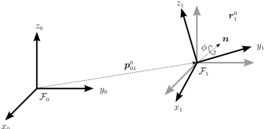
Definition 3.16. LetF0 be a frame that will be rotated of an angleφaround a unit norm axis n=nxˆı+nyˆ+nzˆk, andF1 be the resultant frame after the rotation. This rotation with respect to F0 is represented by the unit norm quaternion r01 given by

r0 1= cos

_φ

2

+nsin

_φ

2

. (3.16)

Letting φ= 0◦ _{we obtain a null rotation, which is equal to}₁_.

Given the quaternion rj

i representing a rotation from the frame Fj to Fi,2 and the

quaternion pi _{representing a point in} _F

i, the projection ofpi in the frame Fj, given by pj,

is expressed by

pj₌_rj ip

i₍_rj i)

∗

. (3.17)

Example 3.1. Let r0

1 and p 0

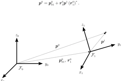
01 be quaternions representing, respectively, the rotation and translation from the frameF0 to F1, as depicted in Figure 3.1. The pointp1 with respect to F1, when represented with respect toF0, is computed by

p0₌_p0 01+r

0 1p

1₍_r0 1)

∗

.

F0

F1 z0

y0

x0

z1

y1

x1

p0 01,r

0 1

p1

p0

Figure 3.1: Example of the projection of a point.

Gait and balance kinematic control for a humanoid robot based on dual quaternion algebra

m

α

cr

φ

@ufmg

GAIT AND BALANCE KINEMATIC CONTROL

FOR A HUMANOID ROBOT BASED ON DUAL

QUATERNION ALGEBRA

GAIT AND BALANCE KINEMATIC CONTROL

FOR A HUMANOID ROBOT BASED ON DUAL

QUATERNION ALGEBRA

Acknowledgements

Resumo

Abstract

Contents

List of Figures

List of Tables

Acronyms

Notation

1

Introduction

1.1

Historical Background

1.2

Objectives

1.3

Contributions

1.4

Structure of the Text

2

State of the Art

2.1

Modeling of Biped and Humanoid Robots

2.2

Walking Pattern

2.3

Control of Gait and Balance

2.4

Chapter Overview

3

Mathematical Background

3.1

Basic Concepts in Dual Quaternion Theory

3.1.1

Quaternions

3.1.2

Dual Quaternions

3.2

Dual Quaternions Representing Rigid Motions

3.2.1

Rotations and Translations Represented by Quaternions