m
α
cr
φ
@ufmg
Universidade Federal de Minas Gerais
Programa de P´os-Gradua¸c˜ao em Engenharia El´etrica
MACRO Research Group - Mecatronics, Control and Robotics
WHOLE-BODY CONTROL OF A MOBILE
MANIPULATOR USING FEEDBACK
LINEARIZATION AND DUAL QUATERNION
ALGEBRA
Frederico Fernandes Afonso Silva Belo Horizonte, Brazil
Frederico Fernandes Afonso Silva
WHOLE-BODY CONTROL OF A MOBILE
MANIPULATOR USING FEEDBACK
LINEARIZATION AND DUAL QUATERNION
ALGEBRA
Dissertation submitted to the Programa de P´os-Gradua¸c˜ao em Engenharia El´etrica of Escola de En-genharia at the Universidade Federal de Minas Gerais, in partial fulfillment of the requirements for the degree of Master in Electrical Engineering.
Advisor: Bruno Vilhena Adorno
Acknowledgements
Two years go fast, so much happens in between though. A master’s degree has this accelerated pace and I would like to thank everyone that stayed by my side during this journey, not forgetting the ones that just arrived in my life alongside the road. Especial thanks to my parents, Flavio and Isabel, for the constant support and incentive. I would not be here without you. To my brother, Lucas, for all the laughs and company to movie marathons (specially the found footage ones).
My deepest thanks to Prof. Bruno Adorno, who has been advising me since the end of my undergraduate course. He has been a model of professionalism, ethics and management ever since. Always present in the work, in both the theoretical and practical aspects of it. I owe him a great deal of my capabilities of critical thinking, writing and work presentation. I am very grateful for all the “just five minutes” meetings, in which he would always find time in the middle of his attributions to pointing me in the right direction.
Thank you to all the UFMG’s staff, for helping in my academic formation during this degree. Specially to Prof. Guilherme Raffo, Prof. Luciano Pimenta and Prof. Leonardo Tˆorres, for being models of professionalism. Thank you to Vera, for never stressing with our mess in the laboratory and for always keeping things in order for us, always smiling. A especial thanks to Prof. Guilherme Raffo, for hosting the best event of the year: the annual MACRO’s barbecue! He honors the traditions of the “Brazilians of the South,” with the best meats and the coldest beers!
Thanks to all my friends that endured the moments of despair at the end of disciplines and papers’ deadlines, without never giving up. Thank you to Gabriela (Gabi), Stella, Rafael, Diana, Fredy, Juan (Juancho), Daniel, Brenner, Arturo, Marcelo, Mariana (Mari), Let´ıcia and Edson, for keeping the laboratory this great place to work in. Thanks also to the friends of the neighbor laboratory, Marcus, Petrus and Wendy, who never said no to a beer.
Finally, a very especial thanks to B´arbara, who, despite being in my life only since the beginning of the year, is teaching me the meaning of partnership, trust and how it is to have someone that is truly there for you.
Agradecimentos
Dois anos passam r´apido, mas tanto acontece nesse tempo. O mestrado tem um ritmo acelerado e eu gostaria de agradecer a todos aqueles que permaneceram ao meu lado durante essa jornada, sem esquecer daqueles que vieram a fazer parte da minha vida ao longo do caminho. Um agradecimento especial aos meus pais, Flavio e Isabel, por sempre me apoiar e incentivar. Eu n˜ao estaria aqui sem vocˆes. Ao meu irm˜ao, Lucas, por todas as risadas e maratonas de filmes (especialmente os found footage).
Meus mais sinceros agradecimentos ao Prof. Bruno Adorno, que vem me orientando desde o final da minha gradua¸c˜ao. Ele vem sendo um modelo de profissionalismo, ´etica e administra¸c˜ao desde ent˜ao. Sempre presente nos trabalhos, tanto nos aspectos te´oricos quanto nos pr´aticos. Eu lhe devo grande parte das minhas habilidades de pensamento cr´ıtico, escrita e apresenta¸c˜ao de trabalhos. Sou muito grato por todas as reuni˜oes de “apenas cinco minutinhos”, onde ele sempre encontrava tempo em meio `as suas atribui¸c˜oes
para me apontar a dire¸c˜ao correta.
Obrigado a todos os funcion´arios da UFMG, por terem ajudado na minha forma¸c˜ao acadˆemica. Um agradecimento especial aos professores Guilherme Raffo, Luciano Pimenta e Leonardo Tˆorres, por serem modelos de profissionalismo. Obrigado `a Vera, por nunca se estressar com as nossas bagun¸cas no laborat´orio e sempre manter tudo organizado para a gente, sempre sorrindo. Um agradecimento especial ao Prof. Guilherme Raffo, por sediar o melhor evento do ano: o churrasco anual do MACRO! Ele honra as tradi¸c˜oes dos “brasileiros do sul”, com as melhores carnes e as cervejas mais geladas!
Obrigado a todos os meus amigos que suportaram os momentos de desespero de final de disciplinas e datas finais de artigos, sem nunca desistir. Obrigado Gabriela (Gabi), Stella, Rafael, Diana, Fredy, Juan (Juancho), Daniel, Brenner, Arturo, Marcelo, Mariana (Mari), Let´ıcia e Edson, por manterem o laborat´orio esse ´otimo lugar para se trabalhar.
Obrigado tamb´em aos amigos do laborat´orio vizinho, Marcus, Petrus e Wendy, que nunca negaram uma cervejinha.
Finalmente, um agradecimento muito especial `a B´arbara, que, apesar de estar na minha vida apenas desde o come¸co do ano, vem me ensinando o significado de companheirismo, confian¸ca e como ´e ter algu´em verdadeiramente ao seu lado.
Resumo
Essa disserta¸c˜ao de mestrado apresenta o controle de corpo completo de um manipulador m´ovel n˜ao-holonˆomico utilizando controle por realimenta¸c˜ao entrada-sa´ıda e ´algebra de quat´ernios duais. O controlador, cuja referˆencia ´e um quat´ernio dual unit´ario representando a pose desejada do efetuador, age como um gerador dinˆamico de trajet´oria para o efetuador, e os sinais de entrada tanto para a base m´ovel n˜ao-holonˆomica quanto para o bra¸co manipulador s˜ao gerados utilizando a pseudo-inversa da matriz Jacobiana de corpo completo. Para lidar com as restri¸c˜oes de n˜ao-holonomia, o sinal de entrada para a base m´ovel gerado pelo controle de corpo completo ´e devidamente remapeado para garantir factibilidade. Restri¸c˜oes nos limites das juntas, existentes na plataforma real, s˜ao tratadas como restri¸c˜oes na matriz Jacobiana. A estabilidade de Lyapunov para o para o sistema em malha fechada ´e apresentada, utilizando o m´etodo direto de Lyapunov e o teorema de Matrosov, e resultados experimentais em uma plataforma real s˜ao realizados para comparar o esquema proposto com um controlador cinem´atico tradicional de corpo completo. Os resultados mostram que, para uma taxa de convergˆencia similar, o controlador n˜ao linear ´e capaz de gerar movimentos mais suaves, al´em de possuir menor esfor¸co de controle do que o controlador linear.
Palavras-chave: Controle n˜ao linear, realimenta¸c˜ao entrada-sa´ıda, controle cin-em´atico, manipulador m´ovel n˜ao-holonˆomico, quat´ernios duais.
Abstract
This master thesis presents the whole-body control of a nonholonomic mobile manipulator using feedback linearization and dual quaternion algebra. The controller, whose reference is a unit dual quaternion representing the desired end-effector pose, acts as a dynamic trajectory generator for the end-effector, and input signals for both nonholonomic mobile base and manipulator arm are generated by using the pseudoinverse of the whole-body Jacobian matrix. In order to deal with the nonholonomic constraints, the input signal to the mobile base generated by the whole-body motion control is properly remapped to ensure feasibility. Joint constraints, which are present in the real platform, are treated by means of constraints in the Jacobian matrix. The Lyapunov stability for the closed-loop system is presented, utilizing Lyapunov’s Direct Method and Matrosov’s theorem, and experimental results on a real platform are performed in order to compare the proposed scheme to a traditional classic whole-body linear kinematic controller. The results show that, for similar convergence rate, the nonlinear controller is capable of generating smoother movements while having lower control effort than the linear controller.
Keywords: Nonlinear control, feedback linearization, kinematic control, nonholonomic mobile manipulator, dual quaternions.
Contents
List of Figures x
List of Tables xiii
Acronyms xiv
Notation xv
1 Introduction 1
1.1 Objective and Contributions . . . 2
1.2 Dissertation Outline . . . 3
2 State of the Art 4 2.1 Whole-body Control . . . 4
2.2 Control of Nonholonomic Mobile Manipulators . . . 7
2.3 Nonlinear Control in Robotics . . . 9
2.4 Joints’ Constraints . . . 11
2.5 Chapter Conclusions . . . 12
3 Mathematical Background 13 3.1 Dual Quaternion Algebra . . . 13
3.1.1 Quaternions . . . 13
3.1.2 Dual Quaternions . . . 14
3.1.2.1 Unit Dual Quaternions . . . 15
3.2 Lyapunov’s Theory . . . 17
3.2.1 Equilibrium Points . . . 18
3.2.2 Lyapunov’s Stability . . . 18
3.2.2.1 Lyapunov’s Direct Method . . . 19
3.2.3 Matrosov’s Theorem . . . 19
3.3 Chapter Conclusions . . . 20
CONTENTS ix
4 Whole-body Modeling and Control 21
4.1 Whole-body kinematics of Mobile Manipulators . . . 21
4.1.1 Manipulator Kinematics . . . 22
4.1.2 Mobile Base Kinematics . . . 23
4.1.3 Whole-body Kinematics . . . 24
4.2 Nonlinear Controller Design . . . 24
4.2.1 Error dynamics for the end-effector pose . . . 25
4.2.2 Design of the feedback linearizing control law for the end-effector pose 26 4.2.3 Whole-body controller . . . 27
4.2.4 Stability analysis of the end-effector closed-loop dynamics . . . 29
4.3 Classic linear kinematic control . . . 33
4.4 Modified Jacobian Clamping . . . 33
4.5 Chapter Conclusions . . . 34
5 Experiments and Results 35 5.1 Experimental Setup . . . 35
5.2 Results . . . 36
5.2.1 Effects of the Nonlinear Controller Gains . . . 36
5.2.2 Comparison of Controllers . . . 37
5.2.3 Joints’ Constraints . . . 40
5.2.3.1 Simulations . . . 40
5.2.3.2 Experiments in the Real Robot . . . 42
5.3 Chapter Conclusions . . . 45
6 Conclusion and Future Works 48
List of Figures
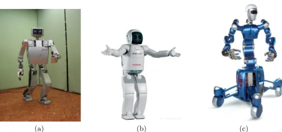
2.1 Robots used in works on whole-body control: (a) H7 (Nishiwaki et al., 2005); (b) ASIMO (courtesy of Honda); (c) Justin (courtesy of DLR). . . 6
3.1 Three-dimensional position(px, py, pz)being represented by the pure
quater-nion p= ˆıpx+ ˆpy + ˆkpz. . . 14
3.2 Rotation of an angle φ around a rotation axis nbeing represented by the rotation quaternion r = cos (φ/2) +nsin (φ/2). . . 15 3.3 Sequence of rigid transformations represented by unit dual quaternions. . . 16 3.4 Lyapunov’s concepts of stability (Slotine and Li, 1991). . . 18 3.5 Intuition behind the Matrosov’s Theorem. As the function W˙2 (solid blue
curve) is upper bounded by a definite negative function −ω (red dot-dashed
curve), lim
t→∞
˙
W2 = 0. . . 20
4.1 Mobile manipulator composed of a nonholonomic mobile base serially at-tached to a 5-DOF manipulator arm. . . 22 4.2 Differential-drive mobile base. In order to deal with the nonholonomic
con-straint, a change in the reference coordinate system is performed. Therefore, the coordinate system is transferred from the center (x, y) to a displaced point (xd, yd). . . 23
4.3 Overall scheme for the whole-body pose control of the nonholonomic mobile manipulator . . . 24
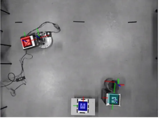
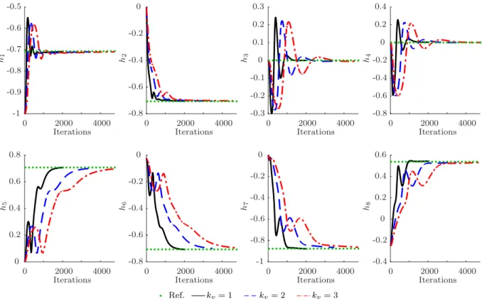
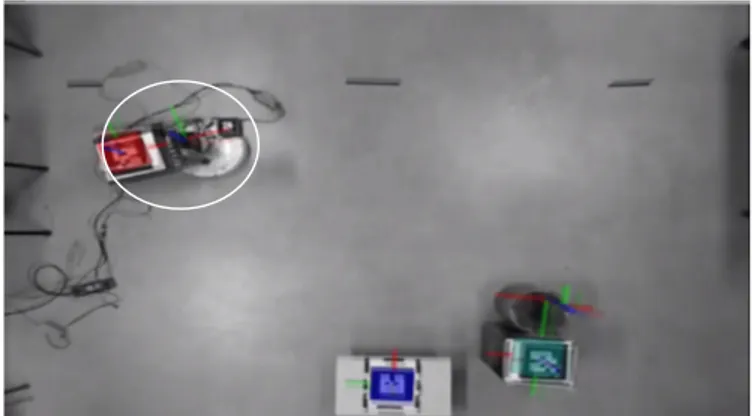
5.1 In the test scenario, the goal consisted of moving a small cube to a desired location and then dropping it into a basket. Both the robot’s end-effector pose and the pose of the goal were measured in real time by using a Kinect sensor located at the ceiling and fiducial markers. . . 36 5.2 Coefficients of the dual quaternion corresponding to the end-effector pose.
Thedotted green curve corresponds to the desired pose and in all experiments ¯
kp = 0.6. The solid black curve corresponds to kv = 1, the blue dashed
curve corresponds to kv = 2, and the red dot-dashed curve corresponds to
kv = 3. . . 37
LIST OF FIGURES xi
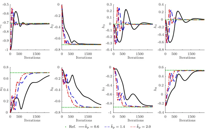
5.3 Coefficients of the dual quaternion corresponding to the end-effector pose. Thedotted green curve corresponds to the desired pose and in all experiments
kv = 2. The solid black curve corresponds to ¯kp = 0.6, the blue dashed
curve corresponds to ¯kp = 1.4, and the red dot-dashed curve corresponds to
¯
kp = 2. . . 38
5.4 Snapshots from the experiments, where the executed trajectories from both controllers are superimposed. The semi-transparent robot (marked with a white circle) shows the motion generated by the classic controller (4.46) and the regular (not transparent) robot shows motion generated by the nonlinear controller (4.27). . . 39 5.5 Coefficients of the dual quaternion error. The red dot-dashed curve
corre-sponds to the nonlinear controller whereas the solid blue curve corresponds to the classic linear kinematic controller. . . 40 5.6 Euclidean norm the end-effector pose error (kvec8(1−x˜)k). The red
dot-dashed curve corresponds to the nonlinear controller whereas the solid blue
curve corresponds to the classic linear kinematic controller. . . 41 5.7 Control inputs (joints velocities). The red dot-dashed curve corresponds
to the nonlinear controller whereas the solid blue curve corresponds to the classic linear kinematic controller. . . 41 5.8 Snapshots from the simulation of the Jacobian Clamping in Matlab. . . . 43 5.9 Coefficients of the dual quaternion corresponding to the end-effector pose.
The greyish area of the graph indicates the phase in which the robot is trying to converge to a pose that is unreachable without violating the joints’ limits. The solid black curve correspond to the desired pose of the nonlinear controller. The red dot-dashed curve corresponds to the nonlinear controller without the use of Jacobian Clamping whereas the dashed blue
curve corresponds to the nonlinear controller with the use of Jacobian Clamping. . . 44 5.10 Joint angles. Thesolid black curve correspond to the joints’ limits. Thered
dot-dashed curve corresponds to the nonlinear controller without the use of Jacobian Clamping whereas the dashed blue curve corresponds to the nonlinear controller with the use of Jacobian Clamping. . . 44 5.11 Snapshots from the experiments, where the executed trajectories from both
LIST OF FIGURES xii
5.12 Coefficients of the dual quaternion corresponding to the end-effector pose. The vertical dashed black line indicates the moment in which the motor stopped working and the experiment was interrupted. The solid black
curve correspond to the desired pose of the nonlinear controller. The red dot-dashed curve corresponds to the nonlinear controller without the use of Jacobian Clamping whereas the dashed blue curve corresponds to the nonlinear controller with the use of Jacobian Clamping. . . 47 5.13 Joint angles. The solid black curve correspond to the joints’ limits. The
List of Tables
5.1 Control Effort. Comparison of the control effort for all controllers . . . 40
Acronyms
ASIMO Advanced Step in Innovative MObility
CDTS Cooperative Dual Task-Space.
DLR German Aerospace Center.
DOF Degrees of Freedom.
JINT Journal of Intelligent & Robotic Systems.
LARS Latin American Robotics Symposium.
ROS Robot Operating System.
SBR Brazilian Robotics Symposium.
UAV Unmanned Aerial Vehicle.
Notation
H Set of quaternions.
H Set of dual quaternions.
I Identity matrix.
ˆı,ˆ,ˆk Imaginary units.
J† Damped pseudoinverse.
JT Transpose of J.
J Jacobian matrix.
p×q Cross product between dual quaternions pand q. D
p,qE Dot product between dual quaternions pand q.
R Set of real numbers.
Spin(3) Tridimensional spin group.
x∗ Conjugate of dual quaternion x.
˜
x Error related to dual quaternion x.
˙
x Time derivative of x.
ε Dual unit.
Lowercase bold letters represent column vectors or quaternions:
a =
a1
...
an
, a ∈R
n
LIST OF TABLES xvi
or
b=b1+ ˆıb2+ ˆb3+ ˆkb4, b ∈H.
Uppercase bold letters represent matrices:
A=
a11 · · · a1m
... ... ...
an1 · · · anm
, A∈R
n×m
.
Underlined variables represent dual numbers:
a=a1+εa2, a ∈ H,
whereas
h=h1+εh2, h∈ H
1
Introduction
Over the last years, humanoids and mobile manipulators have attracted increasing attention in academic research, thanks to the versatility offered by such platforms. They can be used in many daily tasks such as, for example, picking up a cup (Salazar-Sangucho and Adorno, 2014), interacting with objects in shelves (Dalibard et al., 2013), entertainment (Ishida, 2004) and personal assistance (Meeussen et al., 2010; Chen et al., 2013). When interacting with humans, specially in tasks of rehabilitation, it is often undesirable (if not prejudicial) that the robot present abrupt movements (Alcocer et al., 2012; Lasota et al., 2014). In order to allow fluid and human-like movements, a strategy of whole-body motion—i.e., motions that use all available degrees of freedom (DOF)—may be used to control both humanoids and mobile manipulators.
Although humanoids are the first type of robots that may come to mind when one thinks about robots for human environments, such robots present extra challenges in the control. For instance, let us assume a simple task of picking up an object that is out of the robot’s reach. In addition the proper control focused on performing the desired task, humanoids also need to perform simultaneously other tasks, such as, for example, balance and gait control. Another drawback in the usage of humanoids lies in the fact that the majority of these robots are very expensive.
On the other hand, mobile manipulators combine the dexterity of robotic arms with the mobility of mobile bases, being a versatile and low cost option to work in human environments. Another advantage of these platforms is that they do not need balance control, as the base is naturally in equilibrium. Nevertheless, one of the most common
CHAPTER 1. INTRODUCTION 2
mobile bases is the differential mobile base, which presents the challenge of being a first order nonholonomic system (i.e., it has restrictions in the instantaneous velocities that it may execute).
Classic approaches to control mobile manipulators consists of controllers whose control effort is proportional to the error. Therefore, when the error is to large (e.g., the robot end-effector starts far from its desired pose) the robots presents abrupt movements. In order to mitigate this problem, this work explores the development of a nonlinear control technique.
In order to control the end-effector pose (i.e., position and orientation) a suitable representation should be used. Dual quaternions are one good example, since they are more compact and computationally efficient than homogeneous transformation matrices and also do not present representational singularities (Adorno, 2011). In addition, dual quaternions can be used to represent rigid motions, twists, wrenches, and several geometric primitives (e.g., Pl¨ucker lines, planes, etc.) (Adorno, 2017). Thanks to their strong algebraic properties, different robots can be modeled using the same systematic procedure (e.g., single or cooperative manipulators (Adorno et al., 2010), mobile manipulators (Adorno, 2011), and humanoids (Oliveira and Adorno, 2015; Fonseca and Adorno, 2016)), and the resultant models can be directly used with standard kinematic controllers without the need of any intermediate parameterization (Pham et al., 2010; Adorno et al., 2010; Figueredo et al., 2013). Thanks to those aforementioned advantages, dual quaternion algebra is the main mathematical tool used in this dissertation for robot modeling and control.
Real platforms often present limitations in the angles that its joints may assume. If this aspect is not considered during the controller’s design and is not properly treated, it may potentially leads to instability of the system. Therefore, this work explores some existent techniques that aim to solve such problem.
1.1
Objective and Contributions
This work has as main objectives the design and implementation of a nonlinear kinematic controller for the whole-body control of a nonholonomic mobile manipulator. The motiva-tion behind the usage of a nonlinear control lies in the desire to mitigate the abrupt initial movement presented by classic approaches of kinematic control (i.e. controllers whose control effort is proportional to the error), when the initial error is too large.
CHAPTER 1. INTRODUCTION 3
and Adorno (2014).
The main contribution of this master’s thesis is the development of a whole-body control strategy for a first order nonholonomic mobile manipulator using feedback linearization and dual quaternion algebra. Although feedback linearization has already been developed for pose control using dual quaternion algebra (Wang and Yu, 2013), those techniques combined have never been adapted and applied to first order nonholonomic mobile manipulators. In addition, this dissertation has the following novel contributions
❼ The nonlinear dynamical controller proposed by Wang and Yu (2013) was adapted to a nonlinear kinematic controller, extending its applicability to robots actuated on velocity or joint position (e.g. the majority of commercial mobile manipulators);
❼ Removal of the cascade structure proposed by Salazar-Sangucho and Adorno (2014), ensuring feasible control inputs to the nonholonomic mobile base by means of a suitable input mapping (see Section 4.2.3);
❼ Formal stability proof of the end-effector closed-loop dynamics, using Lyapunov’s Direct Method and Matrosov’s Theorem (see Section 4.2.4);
❼ Modification of the Jacobian Clamping (Colome and Torras, 2015), removing its limitation of permanently blocking a joint and allowing the robot to potentially regain a lost degree of freedom.
The main contributions of this dissertation were accepted with minor revisions by the Journal of Intelligent & Robotic Systems (JINT) and the paper is currently under revision.
1.2
Dissertation Outline
2
State of the Art
This chapter presents a review of important works regarding whole-body control of humanoids and mobile manipulators and, also, nonlinear control in robotics. Techniques to deal with joints’ constraints are also discussed in this chapter. It is divided in four sections: Section 2.1 presents a review of whole-body control, Section 2.2 reviews some control techniques of nonholonomic manipulators and Section 2.3 presents some works related with the use of nonlinear control in robotics. Section 2.4 reviews works with techniques to deal with joints’ constraints.
2.1
Whole-body Control
Whole-body control is defined as a control technique in which all available degrees of freedom (DOF) of a robot are used at once to perform a given task. Usually, in this type of control, the goal is defined in the task space (e.g., a desired pose for the end-effector) and finding suitable joint positions to achieve it, is the task of the controller.
Nishiwaki et al. (2005) proposed a control strategy for the whole-body motion of a humanoid robot for the task of opening a crank while walking continuously. The strategy consists in first determining a desired hand position and, afterwards, deciding torso position and posture according to the position of the hand and the feet. Then, using the calculated torso and hand positions, the inverse kinematic of the arm is used to find the appropriate joint angles. Also, null space control was used to avoid joint constraints, by making the joint which is nearest to its limit farther from the limitation. The proposed control scheme
CHAPTER 2. STATE OF THE ART 5
was tested on the humanoid robot H7 (see Fig. 2.1a).
Sentis and Khatib (2006) proposed a whole-body control framework based on priori-tization of tasks consisting of three hierarchical levels, where constraint-handling tasks have highest priority, followed by operational tasks, and finally posture-optimizing tasks. The tasks with lower priority are projected into the null space of the higher priority tasks. Therefore, this strategy ensures that the constraints will never be violated. The framework was tested only in simulation.
Gienger et al. (2006) presented a control algorithm that allows “displacement intervals” in task space (i.e., valid regions around a given task variable), which are exploited to satisfy one or several cost functions, similar to how redundant control techniques exploit the null space. The strategy was demonstrated through simulation and was also implemented on the humanoid robot Asimo (see Fig. 2.1b).
Nagasaka et al. (2010) proposed a whole-body cooperative force control strategy, known as Generalized Inverse Dynamics, for a mobile manipulator that can achieve different control objectives and interact with both humans and objects while performing whole-body motions. The authors also proposed a hardware configuration, called Idealized Joint Unit, to ensure accurate response to the required torque according to virtual impedance properties (inertia and viscosity). The strategy was tested on a two-armed and two-wheeled robot with 21 DOF.
Pham et al. (2010) proposed a strategy to regulate the end-effector pose of manipulator robots, which is represented by a unit dual quaternion, and uses the pseudoinverse of the robot Jacobian to generate the velocity inputs for the robot joints. By representing position and orientation in a single element, the design of the controller was simplified. The proposed scheme was tested on a six-link manipulator showing the efficiency of the method.
Dietrich et al. (2011) proposed a whole-body impedance-based controller to the DLR’s mobile manipulator Justin (see Fig. 2.1c), which has two arms and a holonomic base. A synchronized behavior was achieved through the use of one single Jacobian for the whole system, except for the hands, and the approach was tested on the real platform.
Adorno (2011) presented an extension of the cooperative dual task-space (CDTS) proposed in Adorno et al. (2010) and evaluated the resultant control strategy through the simulation of a two-arm mobile manipulator for the task of pouring water. The whole-body model developed by Adorno was used in Salazar-Sangucho and Adorno (2014) to implement the whole-body control of a first order nonholonomic mobile manipulator in the task of picking and delivering a bottle of water. Park and Lee (2013) proposed a whole-body motion balance for humanoids robots based on the CDTS and evaluated the strategy by means of simulations.
Figueredo et al. (2013) proposed aH∞ robust controller using dual quaternion algebra
CHAPTER 2. STATE OF THE ART 6
(a) (b) (c)
Figure 2.1: Robots used in works on whole-body control: (a) H7 (Nishiwaki et al., 2005); (b) ASIMO (courtesy of Honda); (c) Justin (courtesy of DLR).
whereas ensuring convergence. A novel error metric in dual quaternion algebra, which is invariant with respect to coordinate changes, was introduced. Simulations highlighted the effectiveness of the proposed strategy in therms of its robustness and performance.
Marinho et al. (2015) proposed an optimal controller to efficiently balance the end-effector error and its task-space velocity, using dual quaternion algebra. Departing from the invariant error definition (Figueredo et al., 2013), they derived a perturbed time-varying linear system and then proposed an optimal criterion strategy to control the error in relation to perturbations, caused by a time-varying trajectory. The strategy was tested through simulation and compared with techniques using a proportional gain controller with and without feed-forward, demonstrating the efficiency of the former in following the trajectory.
Mello et al. (2016) presented a cascade control strategy to track a desired trajectory of the end-effector, in the presence of uncertainties, of a aerial manipulator, which is composed of a robotic arm serially coupled to a quadrotor unmanned aerial vehicle (UAV). The control structure has the inner loop composed of a partial feedback linearization controller obtained from Lie derivative and the outer loop is given by a kinematic controller designed through the linear H∞ controller using LMIs. The whole-body kinematic model
of the aerial manipulator is obtained using dual quaternion algebra.
CHAPTER 2. STATE OF THE ART 7
2.2
Control of Nonholonomic Mobile Manipulators
Robotic systems are invariably subjected to a variety of constraints. A wheeled robot has, for instance, the constraint of rolling without slipping. Such constraints, called Pfaffian constraints, can be written in the form (LaValle, 2006)
φ(q,q˙, t) =0, (2.1)
where q is the robot’s configuration. If the constraints in the form of (2.1) can be integrated in such way that they can be written in the form of φ(q, t) = 0, they are then called holonomic constraint. On the other hand, constraints in the form of (2.1) that cannot be integrated are known as first-order nonholonomic constraints. Physically, first-order nonholonomic constraints imply that the robot is unable to achieve some instantaneous velocities. For instance, a wheeled robot, as a conventional car, is incapable of instantaneously moving in a direction normal to its wheels. It is worth noticing that this limitations in the instantaneous velocities do not prevent the robot to achieve any arbitrary pose, they simply imply that a specific set of maneuvers will be required (e.g., parallel parking maneuvers).
Li and Liu (2004) proposed the modeling and control of a mobile manipulator composed of a three-wheeled mobile platform and a four-DOF manipulator. The nonholonomic constraints of the mobile base were taken into account by means of a constraint Lagrangian formulation. To allow the end-effector to follow a given trajectory, the authors designed a model-based controller, which was proved to be asymptotically stable through Lyapunov theory. The model proposed in that paper was then used by Li and Liu (2005) and Liu and Li (2006), where controllers based on fuzzy logic were developed. In both works a fuzzy self-motion planner was used in conjunct with a robust adaptive controller and a robust adaptive neural-network controller, respectively.
CHAPTER 2. STATE OF THE ART 8
Zhang et al. (2012) presented a control scheme in which a teleoperator provided the mobile manipulator’s end-effector with information of desired pose. To find the solution for the redundant system, the authors suggested the modeling as a multi-objective optimization problem. As restrictions for the optimization problem, nonholonomic constraints, joint limit avoidance, singularity removal, maximum manipulability, obstacle avoidance, among others, were used. The developed controller is based on the pseudo-inversion of the robot’s Jacobian and its null space projector. The effectiveness of the strategy was tested through simulation, using a mobile manipulator.
Jia et al. (2014) proposed a whole-body control strategy for a mobile manipulator composed of a mobile base and a robotic arm. The proposed scheme is composed of three levels. In the first one, a desired motion is given to the end-effector by a human operator using a spaceball. Data is sampled from the given motion and used as desired velocity for the end-effector. Finally, this desired trajectory for the end-effector is used to find a desired trajectory for the mobile base and for the manipulator. In the second level, a coordination planner receives information from the system and actively generates instantaneous input signals based on the original motion plan. The third and last level is a coordination controller that computes the joint’s velocities for both the mobile base and the manipulator to achieve the instantaneous output. It is worth noticing that although the coordination controller concatenates both control signals, the mobile base and the manipulator are controlled separately and each one has its own desired trajectory (obtained in the first level). For mobile base control, the nonholonomic constraints are dealt with through a modification of the kinematic model in order to explicit entail the admissible velocities with respect to such constraints.
Salazar-Sangucho and Adorno (2014) presented a control scheme for a mobile manipula-tor using a cascade structure, in which the outermost level consists in a controller based on the pseudoinverse of the Jacobian matrix and the innermost loop explicitly deals with the nonholonomic constraints of the base, by means of a input-output feedback linearization. The strategy was tested in a real platform for the task of picking up and delivering a bottle of water.
CHAPTER 2. STATE OF THE ART 9
2.3
Nonlinear Control in Robotics
Among the several existent nonlinear control strategies, one of the simplest and most used technique is the one called Feedback Linearization. This strategy consists in obtaining the error dynamics and proposing a feedback linearizing control law that will cancel the system’s nonlinearities and lead it to a virtual control law. The virtual control law is then designed in order to impose the desired dynamics into the system. The general framework of a feedback linearizing control law is given by
u=feedback linearization+virtual control law.
Gilbert and Ha (1984) proposed a systematic approach for feedback system design based on a general error expression. They relied on the inverse kinematics to find the desired joint anglesqd(t)once a desired end-effector pose xd(t)is given. Starting from the
nominal model of the manipulator dynamics and using as error
e
q =qd−q,
where q are the current joint angles, the authors obtained a feedback linearizing control law that compensates the nonlinearities of the system and leads the error dynamics to a virtual control law. As virtual control law, the authors suggested the use of a simple PID controller.
Spong and Vidyasagar (1985) presented a control scheme composed of an approximate feedback control law followed by a linear compensator. The feedback linearizing controller was obtained from the error dynamics starting from the nominal model of the manipulator dynamics, while the linear compensator was designed based on the stable factorization approach (Vidyasagar, 1985) to achieve optimal tracking and disturbance rejection.
Wen et al. (1991) studied the attitude control problem of a single free-floating rigid body. The authors discussed a general controller structure in the form of
u=proportional and derivative feedback+feedforward compensation, (2.2)
CHAPTER 2. STATE OF THE ART 10
Following the work of Wen et al. (1991), Wang and Yu (2013) developed a pose controller for a single free-floating rigid body based on feedback linearization and dual quaternion algebra. The authors developed their control law in the form of (2.2), having terms related to the logarithm of the dual quaternion error and to the twist error as proportional and derivative feedback terms, respectively. For the feedforward compensation, the authors relied on the full dynamic model with known parameters. The results of their work were presented through simulation by using the dynamic model of a “flying brick.”
de Almeida and Raffo (2015) proposed a cascade scheme with three input-output feedback linearization blocks to control a Tilt-rotor UAV carrying a suspended load. The two innermost levels control the aircraft’s altitude and attitude. The third level performs path tracking while reduces the load’s swing. The scheme was tested through simulation and compared with a simpler technique that uses the same controllers designed for the first and second level and replaces the third level by PID controllers, which considers the load as a disturbance. The simulations showed that the proposed scheme reduced the load swing, with an improvement of140%, at the cost of a worsening in 20% in the tracking error of the Tilt-rotor.
Rego et al. (2016) presented a leader-follower formation control problem, in which a Tilt-rotor UAV performed path tracking while being followed by other Tilt-Tilt-rotors UAVs. The control scheme consists of a hierarchical structure composed of a formation backstepping controller based on the Cooperative Dual Task-Space (CDTS) proposed by Adorno et al. (2010) and one linear state-feedback D-stable H∞ controller for each Tilt-rotor UAV,
based on its linearized dynamic equations, for individual reference tracking. The proposed structure was compared through simulation with a classic technique that uses a controller based on task-space inverse dynamics for individual reference tracking, instead of the backstepping controller. The results showed that while both schemes have almost the same behavior in a disturbance-free scenario, when disturbances where added to the acceleration signals generated by the formation controller, only the backstepping controller was able to reject them.
CHAPTER 2. STATE OF THE ART 11
reference for an input-output linearizing controller that explicitly takes into account the nonholonomic constraints of the mobile base. The proposed strategy eliminated the abrupt initial movement due to large errors that is characteristic of kinematic controllers based on the pseudoinverse of the robot Jacobian. The proposed whole-body nonlinear controller was implemented on a mobile manipulator composed of a five-DOF robotic arm attached to a three-DOF differential mobile base. No formal proof of stability was presented in this work.
2.4
Joints’ Constraints
Li´egeois (1977) presented a control strategy using gradient projection in order to solve a secondary task in the null space of the primary. He proposed the use of the quadratic form
H(q) = 1
n
n
X
i=1
qi−q¯
¯
q−qimax !2
,
where n is the number of joints of the robot and q¯= (qimax +qimin)/2, with qimax andqimin being the maximum and the minimum value allowed for the jointi, respectively, to make a manipulator draw a circle, while minimizing the deviation of the joints from its mean positions. It is worth noticing that from the value ofH(q)it is impossible to determine if a joint has reached its limit.
Following the work of Li´egeois (1977), Zghal et al. (1990) proposed a kinematic optimization scheme for the control of manipulators with multiples degrees of redundancy, in which the gradient used was given by
H(q) =
n
X
i=1
qimax −qimin (qimax −qi) (qi−qimin)
.
H(q)tends to infinite when approaching a joint limit and has a minimum value at the joint’s mean position, therefore pushing the joints to the center of their ranges.
Chan and Dubey (1995) proposed the use of a weighting matrix to penalize joints approaching their limits. They compared their technique with strategies using gradient projection, showing that the former reduces robot self-motion while ensuring joint limit avoidance, which, on the other hand, cannot be guaranteed by the later, as joint constraints are projected into the null space of the main task.
CHAPTER 2. STATE OF THE ART 12
defining the weighting matrix as a diagonal matrixH, whose elements are given by
hi =
0 ,if qi > qimax or qi < qimin,
1 ,otherwise. (2.3)
This way, any joint that violate its limit is blocked, but the joints are not pushed from their maximum (or minimum) values. If one joint is blocked, the robot loses one degree of freedom, but may continue to converge to the desired pose using the other available DOFs.
2.5
Chapter Conclusions
This chapter presented a review of whole-body control, control of nonholonomic manipula-tors, nonlinear control in robotics and strategies to deal with joints’ constraints. Although the use of feedback linearization and dual quaternion algebra for pose control was already proposed in the work of Wang and Yu (2013), their goal was to control a single free-floating rigid body and they relied in the full dynamical model of it, having torques and forces as control inputs. The modification of the control structure proposed in this master thesis removes the necessity of the dynamical model of the robot, allowing the implementation of the proposed nonlinear controller in robots actuated in velocity or joint position (e.g. the majority of commercial mobile manipulators).
So far the literature has not presented works applying nonlinear control using dual quaternion algebra to first-order nonholonomic mobile manipulators. Besides, to deal with nonholonomic constraints often one relies in either including such constraints directly in the model (or in the programming of the optimization problem) or using a cascade structure. The remapping of the unfeasible control inputs into feasible ones is one of the contributions of this work.
The Jacobian Clamping as proposed by Colome and Torras (2015), although guaran-teeing that the joints’ limits will be respected and being simple to implement, works in such a way that, once a joint is blocked, it remains blocked forever. A modification in the definition of the matrix H proposed in this dissertation allows the joints to be potentially unblocked during the execution of the movements. This way, the robot may regain the lost degree of freedom, extending the convergence capability of the system, which was fairly limited by the original strategy.
3
Mathematical Background
This chapter provides a brief revision of the principal concepts needed to understand this work. Section 3.1 gives an introduction to dual quaternion algebra, its operations and applications in robotics. Section 3.2 provides a summary of basic concepts of Lyapunov’s Theory and the Matrosov’s Theorem (Matrosov, 1962).
3.1
Dual Quaternion Algebra
This master thesis relies on dual quaternion algebra to obtain both the robot kinematics and the corresponding kinematic controllers, and thus this chapter presents some introductory concepts on dual quaternions. For a more complete account on the subject and its application to robotics, please refer to Adorno (2011); Selig (2005).
3.1.1
Quaternions
Quaternions were proposed by Hamilton in the 19th century (Hamilton, 1844, apud Adorno) with the purpose of extending the algebra of complex numbers, and they are elements of the set given by
H,{h1+ ˆıh2 + ˆh3+ ˆkh4 : h1, h2, h3, h4 ∈R andˆı2 = ˆ2 = ˆk2 = ˆıˆkˆ=−1}. (3.1)
Addition and multiplication of quaternions are analogous to their counterparts of real and complex numbers; one must only respect the properties of imaginary unitsˆı,ˆ,kˆ given
CHAPTER 3. MATHEMATICAL BACKGROUND 14
in (3.1). Quaternions whose real part (i.e., the element not multiplied by any imaginary unit) is equal to zero are called pure quaternions.
Pure quaternions are used to represent positions(px, py, pz) in the three-dimensional
space by means of position quaternions
p= ˆıpx+ ˆpy+ ˆkpz, (3.2)
as shown in Fig. 3.1.
ˆı
ˆ
ˆ
k px
pk
pj
Figure 3.1: Three-dimensional position(px, py, pz)being represented by the pure quaternion
p= ˆıpx+ ˆpy + ˆkpz.
Definition 3.1 (Adorno (2017)). The norm of a quaternion h=hr+ ˆıhx+ ˆhy + ˆkhz is
defined as
khk=√hh∗ =√h∗h,
where h∗ =hr−ˆıhx−ˆhy−ˆkhz is the conjugate of h.
Quaternions whose norm is equal to one are called unit quaternions and are used to represent rotations by means of rotation quaternions
r = cos φ 2
!
+nsin φ 2
!
, (3.3)
where φ is the rotation angle around the rotation axis n = ˆınx+ ˆny + ˆknz, knk = 1,
(Selig, 2005), as illustrated in Fig. 3.2.
3.1.2
Dual Quaternions
Clifford extended the algebra of quaternions in 1873 giving rise to dual quaternions (Selig, 2005), which are elements of the set
H ,{hP +εhD : hP,hD ∈H, ε6= 0, ε2 = 0}. (3.4)
Addition and multiplication of dual quaternions are analogous to their counterparts of real and complex numbers; one must only respect the properties of imaginary unitsˆı,,ˆkˆ
CHAPTER 3. MATHEMATICAL BACKGROUND 15
ˆı
ˆ
ˆ
k
n
φ
ˆı
ˆ
ˆk
Figure 3.2: Rotation of an angle φ around a rotation axis n being represented by the rotation quaternion r = cos (φ/2) +nsin (φ/2).
Definition 3.2 (Adorno (2017)). Given a dual quaternion h=hP +εhD, the operators
P(h),hP,
D(h),hD,
(3.5)
provide the primary part and dual part of h, respectively.
Definition 3.3 (Adorno (2011)). The norm of a dual quaternion x=xP +εxD is given
by
kxk=√xx∗ =√x∗x, (3.6)
where x∗ = x∗P +εx∗
D. When applied to quaternions, this norm is equivalent to the
Euclidean norm.
Dual quaternions whose norm is equal to one are called unit dual quaternions.
3.1.2.1 Unit Dual Quaternions
A subset of dual quaternions, theunit dual quaternions, is used to represent poses (position and orientation) in the three-dimensional space and form the group Spin(3)⋉R3 (Selig, 2005). Unit dual quaternions can always be written as (Selig, 2005)
x=r+ε1
2pr, (3.7)
where p and r are given by (3.2) and (3.3), respectively. Alternatively, (3.7) can be rewritten as
x=r+ε1
2rp
b
CHAPTER 3. MATHEMATICAL BACKGROUND 16
wherepb =Ad(r∗)pis the position with respect to the body frame,1and Ad(r∗)p,r∗pr
with r∗ = cos (φ/2)−nsin (φ/2), such that rr∗ =r∗r = 1.
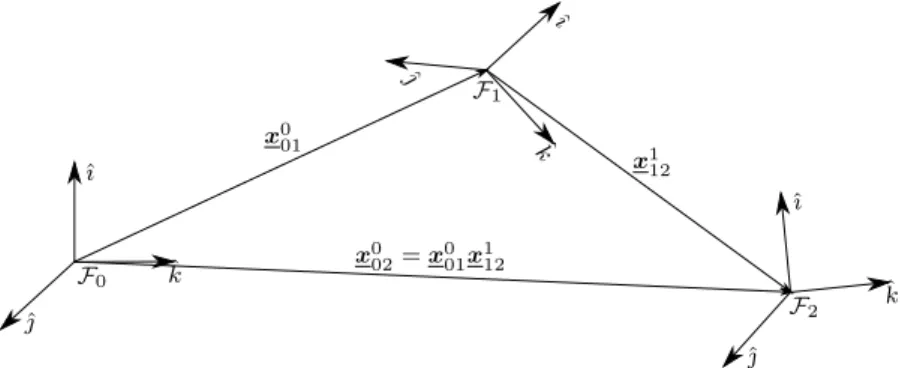
Unit dual quaternions as given by (3.7) or (3.8) can be used to represent a sequence of rigid transformations, wich is done by a sequence of dual quaternion multiplications. Fig. 3.3 shows a sequence of rigid transformations represented by unit dual quaternions.
ˆı
ˆ
ˆ
k
ˆ
ı
ˆ
ˆ
k x0
01
ˆı
ˆ
ˆ
k
x1 12
x0 02=x
0 01x
1 12
F0
F1
F2
Figure 3.3: Sequence of rigid transformations represented by unit dual quaternions.
The time derivative of x is given by (Han et al., 2008)
˙
x= 1
2ξx, (3.9)
where ξ = ω+ε( ˙p+p×ω) is the twist expressed in the inertial frame, with p given by (3.2) andω = ˆıωx+ ˆωy+ ˆkωz is the angular velocity expressed in the inertial frame.
Furthermore,
p×ω , pω−ωp
2 (3.10)
is the cross-product between pure quaternions, which is analogous to the cross product between vectors inR3 and can be verified by direct calculation (Adorno, 2017). In addition, the dot product between two pure quaternions pand q is given by
hp,qi,−(pq+qp)
2 (3.11)
and can also be verified by direct calculation (Adorno, 2017). Alternatively to (3.9),
˙
x= 1 2xξ
b
(3.12)
with ξb = ωb+εp˙b+ωb×pb being the twist expressed in the body frame (Adorno, 2017).
1
CHAPTER 3. MATHEMATICAL BACKGROUND 17
Definition 3.4 (Han et al. (2008)). Given a dual quaternion xas in (3.7), its logarithm is given by
logx= φn 2 +ε
p
2, (3.13)
with inverse mapping given by x= exp (logx)(Adorno, 2011).
Definition 3.5 (Adorno (2017)). The operator vec8 : H 7→R8 gives a bijective mapping
between dual quaternions and an eight-dimensional vector space. More specifically, given
x∈ H such that x=x1+ ˆıx2+ ˆx3+ ˆkx4+ε
x5 + ˆıx6+ ˆx7+ ˆkx8
, then
vec8x=
h
x1 x2 x3 x4 x5 x6 x7 x8
iT
. (3.14)
Definition 3.6. The operator vec
8 : R8 7→ H performs the inverse mapping given by
(3.14). More specifically, givenx∈R8 such that x=hx1 x2 x3 x4 x5 x6 x7 x8
iT
, then
vec
8x=x1+ ˆıx2+ ˆx3+ ˆkx4+ε
x5+ ˆıx6+ ˆx7+ ˆkx8
. (3.15)
The vec8 operator, together with the Hamilton operators +
H(·) and H− (·), are very useful to perform algebraic manipulations. More specifically, givenx,y∈ H the Hamilton operators satisfy (Adorno, 2011)
vec8
xy=H+ (x) vec8y=
−
Hyvec8x,
where
+
H(h)=
+
H4(P(h)) 04
+
H4(D(h)) H+4(P(h)) ,
−
H(h) =
−
H4(P(h)) 04
−
H4(D(h)) H−4(P(h))
, (3.16)
with
+
H4(h) =
h1 −h2 −h3 −h4
h2 h1 −h4 h3
h3 h4 h1 −h2
h4 −h3 h2 h1
, H−4(h) =
h1 −h2 −h3 −h4
h2 h1 h4 −h3
h3 −h4 h1 h2
h4 h3 −h2 h1
.
3.2
Lyapunov’s Theory
CHAPTER 3. MATHEMATICAL BACKGROUND 18
3.2.1
Equilibrium Points
If the system trajectory (i.e., the curve in state space corresponding to the system’s solution) corresponds to a single point, this point is known as equilibrium point.
Definition 3.7 (Slotine and Li (1991)). A state x′ is anequilibrium state (or equilibrium point) of the system if once x(t) is equal to x′, it remains equal to x′ for all future time.
Mathematically, this means that x′ satisfies
f(x′) = 0,
where x˙ =f(x).
3.2.2
Lyapunov’s Stability
Lyapunov’s concept of stability and asymptotic stability are given by the following defini-tions.
Definition 3.8 (Slotine and Li (1991)). The equilibrium point x=0 is said to be stable if, for any R > 0, there exists r > 0, such that if kx(0)k < r, then kx(t)k < R for all
t≥0. Otherwise, the equilibrium point is unstable.
In other words, if the system’s trajectory starts sufficiently close to an equilibrium point and it can be kept arbitrarily close to it, then this equilibrium point is called stable. Such point is also known as marginally stable.
Definition 3.9 (Slotine and Li (1991)). An equilibrium point x = 0 is asymptotically stable if it is stable, and if in addition there exist some r >0such that kx(t)k< rimplies that x(t)→0 ast → ∞.
That is, if the equilibrium point is asymptotically stable, states starting close to it will converge to this equilibrium point ast→ ∞.
The concepts of Lyapunov’s stability and asymptotic stability are illustrated in Fig. 3.4.
CHAPTER 3. MATHEMATICAL BACKGROUND 19
3.2.2.1 Lyapunov’s Direct Method
Lyapunov’s Direct Method consists in finding a function of the states of the system and analyzing its time derivative to determine the stability of the equilibrium point at the origin. The method is stated in the Definition 3.10.
Definition 3.10 (Slotine and Li (1991)). Given a function V (x) of the states of the system, such as
❼ V (x) is differentiable
❼ V (x) is positive definite
❼ V (x)→ ∞ askxk → ∞
if V˙ (x)≤0, then the equilibrium at the origin is globally stable. If V˙ (x)<0, then the equilibrium at the origin is globally asymptotically stable.
The idea behind the method is that V (x) is a “energy-like” function of the dynamic system. Therefore, by analyzing its time derivative it is possible to infer the system behavior.
3.2.3
Matrosov’s Theorem
Originally proposed by Matrosov (1962), a simplified version of Matrosov’s Theorem was presented by Astolfi and Praly (2011) and states that if V˙ ≤0 and there exist two differentiable functions W1, W2 : Rn → R, two continuous and positive semi-definite
functions N1, N2 : Rn → [0,∞), a continuous function ψ : R→R satisfying ψ(0) = 0,
and a positive definite functionω : Rn →
R such that
˙
W1 ≤ −N1,
˙
W2 ≤ −N2+ψ(N1),
ω≤N1+N2,
then the origin is an equilibrium point globally asymptotically stable and all bounded trajectories converge to it. Matrosov’s theorem is usually used in its simplified version (Astolfi and Praly, 2011) by letting W1 , V. In addition, choosing N1 , 0 (which is
clearly differentiable and positive semi-definite), then it is only necessary to choose the appropriate functions W2 and ω such that
˙
W2 ≤ −ω (3.17)
CHAPTER 3. MATHEMATICAL BACKGROUND 20
The intuition behind Matrosov’s Theorem is that, as the functionW˙2 that is related to
the system’s states is upper bounded by the negative definite function −ω,2 lim
t→∞
˙
W2 = 0
independently of its momentarily behavior in the past few instants. Fig 3.5 illustrate this idea.
time
v
a
lu
e
−ω W˙2
Figure 3.5: Intuition behind the Matrosov’s Theorem. As the functionW˙2 (solid blue curve)
is upper bounded by a definite negative function−ω (red dot-dashed curve), lim
t→∞
˙
W2 = 0.
3.3
Chapter Conclusions
This chapter reviewed some fundamental mathematical concepts to this work, such as dual quaternion algebra, Lyapunov Stability and Matrosov’s Theorem. Section 3.1 presented the definitions, operations, properties and applications of dual quaternions in the representation of rigid transformations. Section 3.2 reviewed the concepts of equilibrium point, Lyapunov’s stability and asymptotic stability and presented the Matrosov’s Theorem.
2
4
Whole-body Modeling and Control
This chapter presents the whole-body kinematic modeling of the mobile manipulator and the nonlinear control law proposed in this work. Section 4.1 shows how the whole-body kinematic model is obtained using dual quaternion algebra. Section 4.2 presents the design of the nonlinear control and the stability for the end-effector closed-loop dynamics. Section 4.3 reviews the classic kinematic control, which will be used as base of comparison to evaluate the proposed control scheme.
4.1
Whole-body kinematics of Mobile Manipulators
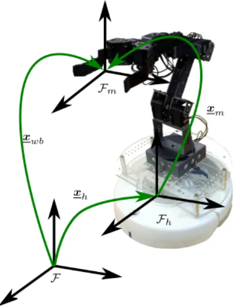
This section briefly presents the whole-body kinematics of the mobile manipulator used in this work (see Fig 4.1), starting from the robot kinematics of each subsystem (i.e. the robot manipulator and the mobile base) to the whole-body model that is used in the final controller. For more details, please refer to (Adorno, 2011).
Furthermore, it is used the mobile base iRobot Create that has three DOF but only two actuations in a differential drive configuration, which results in a first-order nonholonomic system.
CHAPTER 4. WHOLE-BODY MODELING AND CONTROL 22
F
Fh
Fm
xh
xm
xwb
Figure 4.1: Mobile manipulator composed of a nonholonomic mobile base serially attached to a 5-DOF manipulator arm.
4.1.1
Manipulator Kinematics
The forward kinematics of any robot can be represented by a suitable mapping f : Rn→
Spin(3)⋉R3 such that
x=f(q), (4.1)
whereq ∈Rn is the vector of the robot configuration vector and x∈Spin(3)⋉R3 is the
end-effector pose (Adorno, 2011).
This way, given a mobile manipulator composed of a mobile base serially attached to a five-DOF manipulator robot, as shown in Fig. 4.1, the forward kinematics of the robot manipulator is given by
xm =f
m(qm), (4.2)
where qm =hθ1 · · · θ5
iT
is the vector of manipulator joints and xm is the pose of the end-effector with respect to the manipulator base. The corresponding differential forward kinematics is
vec8x˙m =Jmq˙m, (4.3)
where vec8(·) is given by (3.14) andJm ∈R8×5 is the manipulator Jacobian matrix that
CHAPTER 4. WHOLE-BODY MODELING AND CONTROL 23
4.1.2
Mobile Base Kinematics
When used to represent the forward kinematics of a mobile base, the dual quaternion xh
that represents its pose is a function of the Cartesian coordinates(x, y)and the angle φ of the base (Adorno, 2011). Therefore,
xh =rh+
1
2εphrh, (4.4)
with ph = ˆıx+ ˆy and rh = cos (φ/2) + ˆksin (φ/2) .
The forward differential kinematics of the mobile base, without considering the non-holonomic constraints, is given by
vec8x˙h =Jhq˙h, (4.5)
where qh =hx y φiT and Jh ∈R8×3 is the holonomic Jacobian, which is also obtained
algebraically (Adorno, 2011).
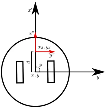
In order to deal with the nonholonomic constraint of the mobile base, a change in the coordinate system is performed (Siciliano et al., 2009), as illustrated in Fig. 4.2. It is easily noticeable that the point (x, y) in the center of the base cannot instantaneously move in the y-axis. However, a displaced point (xd, yd) does not have such constraint and
this fact will be used in the end of Section 4.1 to map the control inputs generated by the whole-body controller into feasible control actions to the mobile base.
x, y xd, yd
x′
y′
x”
y”
d
φ
CHAPTER 4. WHOLE-BODY MODELING AND CONTROL 24
4.1.3
Whole-body Kinematics
The whole-body forward kinematics is given by
xwb=xhxm, (4.6)
where xwb is the end-effector pose with respect to the inertial frame and considers the coupled kinematic chain. The whole-body differential kinematics is given by (Adorno, 2011)
vec8x˙wb =Jwbq˙wb, (4.7)
where qwb =hqT h qTm
iT
and
Jwb =
−
H(xm)Jh
+
H(xh)Jm
,
where H+ (·) and H− (·) are given by (3.16).
4.2
Nonlinear Controller Design
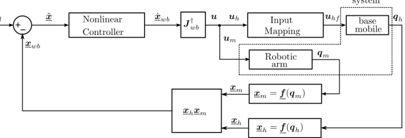
The overall scheme for the whole-body pose control of the mobile manipulator is shown in Fig. 4.3. The reference for the nonlinear controller is a unit dual quaternion representing the desired end-effector pose. The resultant input signal from the nonlinear controller is split into two input signals, one for the manipulator and other for the nonholonomic mobile base. The control signal generated for the latter is properly mapped into feasible inputs to deal with the nonholonomic constraints of the differential mobile base.
xwb
xd x˜ x˙wb
J†wb u uh uhf
qm
xm
xh
um
xm=f(qm)
xh=f(qh)
xhxm
Controller Nonlinear
Mapping Input
mobilebase
Robotic arm
qh
system
CHAPTER 4. WHOLE-BODY MODELING AND CONTROL 25
4.2.1
Error dynamics for the end-effector pose
In order to design the nonlinear controller, first a suitable error in unit dual quaternion space must be defined, such as
˜
x,x∗dxwb
= ˜r +1 2˜rp˜
b
, (4.8)
where xwb=rwb+ε(1/2)rwbpbwb and xd=rd+ε(1/2)rdpbd are the current and desired
end-effector pose, respectively, andr˜= cosθ/˜ 2+nsinθ/˜ 2.
It is important to note that xwb → xd implies x˜ →1, which in turn implies p˜b
→ 0
and ˜r →1. Last, r˜→1 impliesθ˜→0. The time derivative of x˜ is given by
˙˜
x= ˙x∗dxwb+x∗dx˙wb =
1
2xdξ
b d
∗
xwb+x∗d
1
2xwbξ
b wb
=−1 2ξ
b dx
∗
dxwb+
1 2x
∗
dxwbξbwb
=−1 2ξ
b dx˜+
1 2xξ˜
b wb
= 1 2x˜
ξbwb−Ad(˜x∗)ξbd, (4.9)
where Ad(˜x∗)ξb
d,x˜
∗ξb
dx˜, withx
∗ =x∗
P +εx∗D.
Defining
˜
ξb =ξb
wb−Ad(˜x
∗)ξb
d, (4.10)
the time derivative of the dual quaternion error is given by
˙˜
x= 1 2x˜ξ˜
b