EXTRACTING RELATIVE THRESHOLDS FOR
PALOMA MAIRA DE OLIVEIRA
EXTRACTING RELATIVE THRESHOLDS FOR
SOURCE CODE METRICS
Tese apresentada ao Programa de Pós--Graduação em Ciência da Computação do Instituto de Ciências Exatas da Universi-dade Federal de Minas Gerais como req-uisito parcial para a obtenção do grau de Doutor em Ciência da Computação.
Orientador: Marco Tulio Valente
Belo Horizonte
PALOMA MAIRA DE OLIVEIRA
EXTRACTING RELATIVE THRESHOLDS FOR
SOURCE CODE METRICS
Thesis presented to the Graduate Program in Ciência da Computação of the Univer-sidade Federal de Minas Gerais in partial fulfillment of the requirements for the de-gree of Doctor in Ciência da Computação.
Advisor: Marco Tulio Valente
Belo Horizonte
c
2015, Paloma Maira de Oliveira. Todos os direitos reservados.
Oliveira, Paloma Maira de
O48e Extracting Relative Thresholds for Source Code Metrics / Paloma Maira de Oliveira. — Belo Horizonte, 2015
xxiii, 106 f. : il. ; 29cm
Tese (doutorado) — Universidade Federal de Minas Gerais
Orientador: Marco Tulio Valente
1. Computation - thesis. 2. Source Code Metrics. 3. Thresholds. 4. Heavy-tailed distribution. 5. Software Quality. 6. Software Engineer. I. Título.
This thesis is dedicated to my husband Arthur and my parents Ari and Clelia, who has always supported me.
Acknowledgments
This work would not have been possible without the support of many people.
I thank God to provide me the discipline and persistence to reach a Ph.D. degree.
I thank my dear husband Arthur, who has had patience in difficult moments and has always been at my side.
I thank my whole family—especially my father Ari, my mother Clélia, and my sister Fernanda—for having always supported me.
I thank my advisor M. T. Valente for his attention, motivation, patience, dedication, and immense knowledge. I certainly could not complete my Ph.D study without him.
I thank A. Serebrenik for giving me the opportunity to work under his supervision in The Netherlands.
I thank A. Bergel for the valuable collaboration in the case studies.
I thank my colleagues of the IFMG—especially A. F. Camargos, B. Ferreira, D. F. Resende, E. Valadão, F. P. Lima, G. Ribeiro, M. P. Junior, and W. A. Rodrigues—for the friendship and cooperation.
I thank the members of the ASERG research group—especially A. Hora, C. Couto, H. Borges, and L. L. Silva—for the friendship and technical collaboration.
I would like to express my gratitude to the members of my thesis defense—D. Serey (UFCG), E. Figueiredo (UFMG), E. S. Almeida (UFBA), K. A. M. Ferreira (CEFET-MG) and M. A. S. Bigonha (UF(CEFET-MG).
Resumo
Valores de referência confiáveis são necessários para promover o uso de métricas de soft-ware como um efetivo instrumento de medida da qualidade interna de sistemas. Assim, nesta tese de doutorado propõe-se o conceito de Valores de Referência Relativos (VRR) para avaliar métricas que estão em conformidade com distribuições de cauda-pesada (heavy-tailed). Os valores de referência propostos são ditos relativos, pois eles devem ser seguidos pela maioria das entidades de código fonte, contudo tolera-se um número de entidades acima do limite definido. Os VRR são extraídos a partir de um con-junto de sistemas. Descreve-se também uma análise extensiva dos VRR: (i) aplicamos nossos VRR em uma amostra de 308 repositórios disponíveis no GitHub. Conclui-se que a maioria dos repositórios seguem os VRR; (ii) comparamos os VRR propostos com valores de referência extraídos usando um método amplamente usado pela indús-tria de software. Conclui-se que ambos os métodos transmitem informações similares. Contudo, o método proposto detecta automaticamente sistemas que não seguem os VRR; (iii) avaliamos a influência do contexto em nossos resultados e concluímos que o impacto do contexto nos VRR é limitado; (iv) executamos uma análise histórica a fim de verificar se as diferentes versões de um sistema seguem os VRR propostos. Conclui-se que os VRR capturam propriedades de software duradouras; (v) verificamos se classes que não seguem o limite superior de um VRR são importantes. Conclui-se que essas classes são importantes em termos de atividade de manutenção; (vi) inves-tigamos a relação entre presença de bad smells em um sistema e sua aderência com os VRR. Nessa análise, nenhuma evidência foi encontrada; (vii) avaliamos a dispersão dos valores de métricas em sistemas que seguem os VRR usando o coeficiente de Gini. Os resultados mostraram que existem diferentes distribuições de métodos por classe; e (viii) conduzimos um estudo qualitativo para avaliar nosso método com desenvolve-dores. Os resultados indicam que sistemas bem projetados respeitam os VRR e que desenvolvedores geralmente têm dificuldade para indicar sistemas de baixa qualidade.
Palavras-chave: Métricas de código fonte, Valor de referência, Cauda pesada.
Abstract
Meaningful thresholds are needed for promoting software metrics as an effective in-strument to measure the internal quality of systems. To address this challenge, in this PhD Thesis, we propose the concept of Relative Thresholds (RT) for evaluating metrics data following heavy-tailed distributions. The proposed thresholds assume that metric thresholds should be followed by most entities, but that it is also natural to have a number of entities in the “long-tail” that do not follow the defined limits. We describe an empirical method for deriving RT from a corpus of systems. We also perform an extensive analysis of RT: (i) we apply RT on a sample of 308 GitHub repositories. We found that most repositories follow the extracted RT; (ii) We compare the proposed RT with thresholds extracted according to a method used by the software industry. We concluded that both methods convey similar information. However, our method derives RT that can be automatically used to detect noncompliant systems; (iii) we evaluate the influence of context in our results and we concluded that the impact on RT of context changes is limited; (iv) we perform a historical analysis to check whether the proposed RT are followed by different versions of the systems under analysis. We found that our RT capture enduring software properties; (v) we check the importance of classes that do not follow the upper limit of a RT and we found these classes are important in terms of maintenance activities; (vi) we investigate the relation between the presence of bad smells in a system and its adherence to the proposed RT. We do not found evidence that noncompliant systems have more density of bad smells; (vii) we evaluated the dispersion of the metric values in the systems respecting the proposed RT, using the Gini coefficient. We found that there are different distributions of meth-ods per class among the systems that follow the proposed RT; and (viii) We conducted a qualitative study to evaluate our method with developers. The results indicate that well-designed systems respect the RT. In contrast, we observed that developers usually have difficulties to indicate poorly-designed systems.
Keywords: Source code metrics, Thresholds, Heavy-tailed Distributions.
List of Figures
1.1 (a) Histogram of the number of attributes(NOA) for the classes inFindBugs.
(b) Quantile plot for the same data. . . 3
1.2 Relative threshold method . . . 5
2.1 (a) histogram of the populations of all US cities with population of 10 000 or more. (b) another histogram of the same data, but plotted on logarithmic scales. The approximate straight-line form of the histogram in the right panel implies that the distribution follows a heavy-tailed. Data from the 2000 US Census. Figure and caption originally used by Newman et al.[76] 15 3.1 ComplianceRate and ComplianceRatePenalty functions . . . 30
3.2 Compliance Rate Function (NOA metric) . . . 31
3.3 Compliance Rate Penalty Function (NOA metric) . . . 32
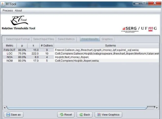
3.4 RTTool stages . . . 37
3.5 Configuration window . . . 38
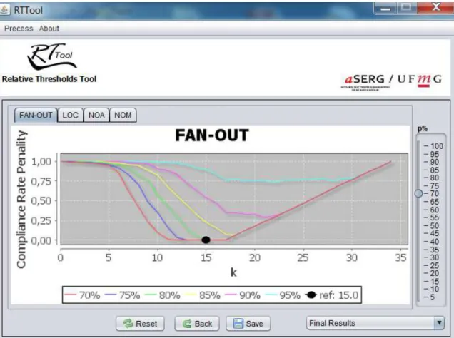
3.6 Final results — with thresholds and noncompliants systems for each metric 39 3.7 ComplianceRate function (FAN-OUT metric) . . . 40
3.8 ComplianceRatePenalty function (FAN-OUT metric) . . . 41
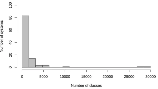
4.1 Size of the systems in the our Corpus . . . 44
4.2 Quantile functions . . . 47
4.3 Percentage of high and very-high risk classes for each system in the Qualitas Corpus. Black bars represent noncompliant systems. . . 54
4.4 Contextual analysis . . . 56
4.5 Contextual analysis for noncompliant systems . . . 57
4.6 Possible states of a class: following or not the upper limit of a relative threshold . . . 58
4.7 Percentage of classes following the upper limit of a relative threshold (pa-rameterk) during the systems’ evolution . . . 60
4.8 Relation between creation and deletion of classes regarding the classes that
do not follow the relative thresholds . . . 62
4.9 Relation between creation and deletion of classes regarding the classes that follow the relative thresholds. In this figure, the percentage of created classes are represented by gray bars, while the percentage of deleted classes are represented by white bars . . . 63
4.10 Percentage of changes in classes that do not follow the upper limits of the relative thresholds proposed for NOM, SLOC, FAN-OUT, RFC, WMC, and LCOM . . . 65
4.11 Number of changes per classes that follow and that do not follow the upper limits of the relative thresholds proposed for NOM, SLOC, FAN-OUT, RFC, WMC, and LCOM . . . 66
4.12 Rate of class-level and method-level bad smells in systems in the Tools subcorpus. The black bars represent noncompliant systems and the gray bars are compliant systems . . . 71
4.13 Inequality Analysis using Gini coefficients . . . 72
4.14 Quantile functions for noncompliants regarding the Gini values . . . 73
5.1 Size of the systems in the PharoCorpus . . . 79
5.2 FAN-OUT quantiles—dashed lines represent PetitParser, PharoLauncher, Pillar, Roassal, and Seaside, which are systems perceived as well-written but that do not follow the relative threshold for FAN-OUT . . . 82
5.3 FAN-OUT example . . . 83
5.4 Gini coefficients . . . 84
5.5 Top-5 maintainers analysis in noncompliant systems . . . 86
5.6 Effort to Maintain (EM) . . . 87
6.1 Percentile plots of scattering degrees (SD). Figure and caption originally used by Queiroz et al. [87] . . . 93
List of Tables
2.1 Source code metric distributions . . . 19
2.2 Source code metric distributions . . . 20
2.3 Thresholds approaches . . . 25
2.4 Thresholds approaches . . . 26
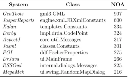
3.1 Classes with highest NOA values . . . 33
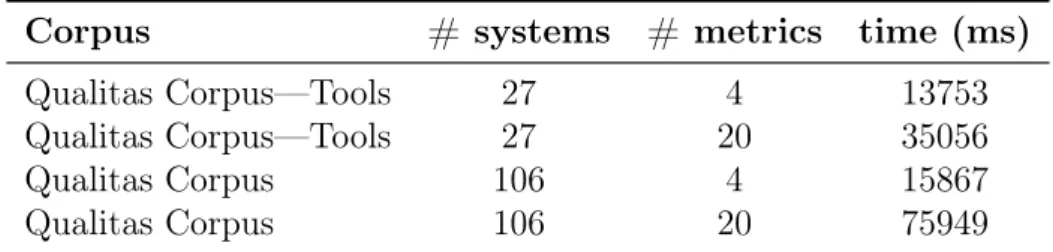
3.2 Runtime of RTTool . . . 40
4.1 Number and percentage of systems with heavy-tailed metric values distri-butions . . . 46
4.2 Relative Thresholds . . . 48
4.3 Top-10 popular GitHub Java repositories (ordered by # stars) . . . 49
4.4 Repositories that follow the proposed relative thresholds . . . 49
4.5 Percentage of classes in the top-10 popular Java repositories that respect the upper limit k of a relative threshold (the underlined value is the only case when a threshold is not respected). . . 50
4.6 Noncompliant repositories for at least three metrics . . . 51
4.7 Relative vs SIG thresholds . . . 52
4.8 Subcorpus by Application Domain . . . 55
4.9 Subcorpus by size . . . 55
4.10 Systems used in the Historical Analysis . . . 59
4.11 Percentage of classes that changed from a state following the upper limit of a threshold to a state not following this limit (ToViolate column) and vice-versa (ToFollow column) . . . 61
4.12 Data on commits log . . . 64
4.13 Top-15 classes with the highest number of changes in Lucene. The table also shows whether each class follow or not the proposed upper limits for the relative thresholds of six metrics . . . 67
4.14 Top-15 classes with the highest number of changes in Spring. The table also shows whether each class follow or not the proposed upper limits for
the relative thresholds of six metrics . . . 68
4.15 Noncompliant systems in theTools subcorpus . . . 69
4.16 Evaluated bad smells . . . 69
5.1 Relative Thresholds for Pharo . . . 80
5.2 Main noncompliant systems . . . 81
5.3 Well-written systems . . . 81
5.4 Percentage of classes in the well-written systems that follow the upper limit k of a relative threshold (underlined values show the cases when the thresh-olds are not respected). . . 82
5.5 Poorly-written systems . . . 84
5.6 Percentage of classes in the poorly-written systems that follow the upper limit k of a relative threshold (underlined values show the cases when the thresholds are violated). . . 85
6.1 Relative thresholds derived by Valeet al. . . 92
Contents
Acknowledgments xi
Resumo xiii
Abstract xv
List of Figures xvii
List of Tables xix
1 Introduction 1
1.1 Motivation . . . 1
1.2 Problem Statement . . . 2
1.3 Goals and Contributions . . . 4
1.4 Thesis Outline . . . 6
1.5 Publications . . . 7
2 Background 9 2.1 Software Quality . . . 9
2.1.1 Software Process Quality . . . 9
2.1.2 Software Product Quality . . . 10
2.2 Source Code Metrics . . . 12
2.2.1 The CK Metrics Suite . . . 13
2.3 Statistical Properties of Source Code Metrics . . . 15
2.3.1 Metrics Values Distributions . . . 17
2.3.2 Discussion . . . 19
2.4 Thresholds Definitions . . . 19
2.4.1 Extracting Thresholds using Traditional Techniques . . . 20
2.4.2 Extracting Thresholds from Repositories . . . 21
2.4.3 Extracting Thresholds using Error Models . . . 23 2.4.4 Extracting Thresholds using Clustering Algorithms . . . 24 2.4.5 Discussion . . . 25 2.5 Studies with Developers . . . 26 2.6 Final Remarks . . . 27
3 Proposed Method 29
3.1 Relative Thresholds . . . 29 3.2 Illustrative Example . . . 31 3.3 Method Properties and Characteristics . . . 33 3.3.1 Adherence to Requirement of Metric Aggregation Techniques . . 33 3.3.2 Staircase Effects . . . 34 3.3.3 Tolerance to Bad Smells . . . 35 3.3.4 Statistical Properties . . . 35 3.4 RTTool . . . 36 3.4.1 Example of usage . . . 37 3.4.2 Performance . . . 39 3.4.3 Availability . . . 40 3.4.4 Related Tools . . . 41 3.5 Final Remarks . . . 41
4 Relative Thresholds for the Qualitas Corpus 43
4.1 Corpus and Metrics . . . 43 4.2 Study Setup . . . 45 4.3 Results . . . 45 4.4 Application on Popular GitHub Repositories . . . 46 4.4.1 Study Setup . . . 48 4.4.2 Results . . . 49 4.5 Comparison with SIG Method . . . 51 4.5.1 Results . . . 52 4.6 Contextual Analysis . . . 53 4.6.1 Study Setup . . . 53 4.6.2 Results . . . 55 4.7 Historical Analysis . . . 57 4.7.1 Study Setup . . . 58 4.7.2 Results . . . 59 4.8 Change Analysis . . . 64
4.8.1 Study Setup . . . 64 4.8.2 Results . . . 65 4.9 Bad Smells Analysis . . . 68 4.9.1 Study Setup . . . 68 4.9.2 Results . . . 69 4.10 Inequality Analysis . . . 72 4.11 Threats to Validity . . . 73 4.12 Final Remarks . . . 74
5 Validating Relative Thresholds with Developers 77
5.1 Study Design . . . 77 5.1.1 Research Questions . . . 77 5.1.2 Corpus and Metrics . . . 78 5.1.3 Methodology and Participants . . . 79 5.2 Results . . . 80 5.2.1 Relative Thresholds for the Pharo Corpus . . . 80 5.2.2 RQ 9: Do systems perceived as well-written by the expert
devel-opers follow the derived relative thresholds? . . . 80 5.2.3 RQ 10: Do systems perceived as poorly-written by the expert
developers do not follow the derived relative thresholds? . . . . 84 5.2.4 RQ 11: Do the noncompliant systems require more effort to
main-tain? . . . 85 5.3 Threats to Validity . . . 87 5.4 Final Remarks . . . 88
6 Conclusion 89
6.1 Summary . . . 89 6.2 Applications of Relative Thresholds . . . 91
6.2.1 A Comparative Study on Metric Thresholds for Software Product Lines . . . 91 6.2.2 Extracting Relative Thresholds for Feature Annotations Metrics 92 6.2.3 Using Relative Thresholds in Industrial Context . . . 94 6.3 Contributions . . . 94 6.4 Further Work . . . 95
Bibliography 97
Chapter 1
Introduction
In this chapter, we start by presenting our motivation (Section 1.1). Next, we present our problem statement (Section 1.2) and an overview of the proposed solution (Sec-tion 1.3). Finally, we present the outline of the thesis (Sec(Sec-tion 1.4) and our publica(Sec-tions (Section 1.5).
1.1
Motivation
With software systems constantly growing in complexity and size, better support is re-quired for measuring and controlling software quality [40]. Essentially, software quality is the degree to which a software meets its requirements [47]. However, evaluating a software system in order to improve its overall quality is not a trivial task. To this purpose, Meyer proposed a set of properties that can be used to evaluate software quality [73]. According to the author, software quality can be evaluated by external factors, i.e., those factors perceived by users, and by internal factors,i.e., those factors only perceived by the development team (developers and maintainers).
Since the inception of the first programming languages, we are witnessing the proposal of a variety of metrics to measure both internal and external quality factors [1, 22, 34, 45, 54, 61]. For example, internal quality factors can be measured by source code metrics, including properties such as modularity, coupling, cohesion, size, inheritance, and complexity. External quality factors include properties such as effi-ciency, correctness, robustness, extensibility, reusability, and ease of use. These metrics provide a quantitative measure of a wide spectrum properties of a software system and they can be used to control the software development and maintenance process. Particularly, software quality managers can rely on metrics to evaluate and control the internal and external quality of a software system, e.g., to certify new components
2 Chapter 1. Introduction
or to monitor the degradation in quality that happens due to software aging. Metrics can also be used to compare and rate the quality of software products, and thus help to define acceptance criteria or service-level agreements between software producers and clients [5, 58]. In spite of such potential benefits of metrics, they are rarely used to control in an effective way the quality of software products [34]. To promote the use of metrics as an effective measurement instrument, it is essential to establish cred-ible thresholds [5, 35, 44, 92]. Metric thresholds are defined by Lorenz and Kidd [67] as:
“Heuristic values used to set ranges of desirable and undesirable metric values for mea-sured software. These thresholds are used to identify anomalies, which may or may not be an actual problem.”
Thresholds have been already defined for many metrics. For example, McCabe pro-posed a threshold value of 10 for his complexity metrics, beyond which a subroutine is deemed unmaintainable and untestable [72]. Another example is that industrial code standards for Java recommend that classes should have no more than 20 methods and that methods should have no more than 75 lines of code [18]. These threshold values are inspired by personal experience and therefore they are not intended as univer-sally applicable. Recently, Alves et al. proposed a more transparent method to derive thresholds from benchmark data [5]. They illustrate the application of the method in a large software corpus and derived, for example, thresholds stating that methods with McCabe complexity above 14 should be considered as very-high risk. However, for most metrics, thresholds are still missing or they do not generalize beyond the context of their inception.
1.2
Problem Statement
The definition of thresholds for source code metric is not a trivial task, because metric values usually follow right-skewed or heavy-tailed distributions [13, 64, 68, 86]. Heavy-tailed distribution are found in many object-oriented properties, describing a common behavior which states that there are few very complex modules while most modules have low complexity [76].
1.2. Problem Statement 3
The histogram is highly right-skewed, meaning that while the bulk of the distribution occurs for fairly small sizes—most classes have few attributes (NOA ≤ 10)—there is a small number of classes with NOA much higher than the typical value, producing the long tail to the right of the histogram. In order to allow an alternative visualization of the full metric distribution, Figure 1.1b depicts the distribution of the NOA values for FindBugs using a quantile plot. The x-axis represents the percentage of observations (percentage of classes) and the y-axis represents the NOA metric values. In Figure 1.1b we can observe that 90% of classes have NOA ≤ 10.
Number of Attributes
FindBugs
0 50 100 150 200
0
200
400
600
800
(a)
0.0 0.2 0.4 0.6 0.8 1.0
0
20
40
60
80
100
Quantiles (% of NOA)
Number Of Atr
ib
uttes
(b)
Figure 1.1. (a) Histogram of the number of attributes(NOA) for the classes in
4 Chapter 1. Introduction
Therefore, in this PhD thesis we assume that in most systems it is “natural” to have source code entities not respecting the existing metric thresholds for several rea-sons, including complex requirements, performance optimizations, machine-generated code, etc. In the particular case of coupling for example, a recent study shows that high coupling can never be entirely eliminated from software design and that in fact some degree of high coupling might be quite reasonable [96].
Existing methods for extracting metric thresholds rely for example on the per-sonal experience of software quality experts [18, 25, 72, 75], on standard statistical measures (e.g., arithmetic mean and standard deviation) [32, 61], machine learning algorithms [44], log transformations [92], and linear regression [14]. There also methods that rely on benchmark for derive thresholds [5, 35]. Thus, a method to define metric thresholds should consider the right-skewed behavior normally observed in source code metric values, as widely reported in the literature.
1.3
Goals and Contributions
We claim in this PhD thesis that metric thresholds should be complemented by a second piece of information, denoting the percentage of entities the upper limit should be applied to. In this context, the main goal of this PhD thesis is to propose and to
validate the concept ofrelative thresholdsfor evaluating source code metrics. Basically, we propose an empirical method to derive relative thresholds based on the analysis of a software corpus. A relative threshold is represented by pairs [p, k] and have the following format:
p% of the entities should have M ≤ k
whereM is a source code metric calculated for a given software entity (method, class,
etc.),kis an upper limit, and pis the minimal percentage of entities that should follow
this upper limit. For example, a relative threshold can state that “80% of the classes should have NOA ≤ 8”. Essentially, this threshold expresses that high risk classes impact the quality of a system whenever they represent more than 20% of the whole population of classes. In other words, the percentage of classes that exceeds the upper limit k do not constitute a threat to the internal quality of the entire project nor an indication of an excessive technical debt [29, 71].
1.3. Goals and Contributions 5
stating that “99% of the classes should have less than 100 attributes” is probably satisfied by most systems in any corpus, it is hardly useful or can be seen as reflecting an acceptable quality principle.
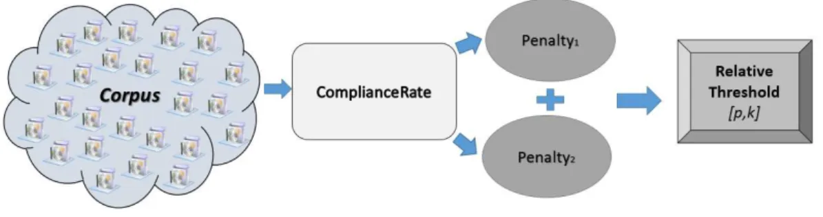
Figure 1.2 presents an overview of our method. Initially, we assume that the values of p and k that characterize a relative threshold for a metric M should emerge
from a curated set of systems, which we call our Corpus. A relative threshold [p, k] is derived using two functions, called ComplianceRate and ComplianceRatePenalty. The function ComplianceRate [p, k] returns the percentage of systems in the Corpus that follow the relative threshold defined by the pair [p, k]. However, this function on its own is not sufficient to optimize p and k. Hence, we introduce the notion of penalties to find the values ofpand k. We penalize a ComplianceRate function in two situations. The first penalty fosters the selection of thresholds followed by at least 90% of the systems in the Corpus. The goal is to derive thresholds that reflect real design rules, which are widely common in the Corpus. Furthermore, ComplianceRate[p, k] receives a second penalty whenever k is greater than metric values that are perceived
as being very high. Finally, the ComplianceRatePenalty function is the sum of penalty1[p, k] and penalty2[k]. A derived relative threshold is the one with the lowest
ComplianceRatePenalty[p, k]. A detailed description of our method is presented in the Chapter 3.
Figure 1.2. Relative threshold method
6 Chapter 1. Introduction
who are the right experts to check whether metric thresholds are indeed able to infer maintainability and design problems.
1.4
Thesis Outline
This thesis is structured in the following chapters:
• Chapter 2 provides a general discussion on software quality and source code met-rics. This chapter also presents related work to our research, such as statistical properties of source code metrics and methods to derive source code metrics thresholds.
• Chapter 3 presents our method to extract relative thresholds from the measure-ment data of a benchmark of software systems. An illustrative example of the proposed method is also presented. Finally, the chapter discusses some aspects and properties of the proposed method. We conclude by presenting RTTool, an open source tool that automates our method.
• Chapter 4 reports an extensive evaluation, through which we apply our method to extract relative thresholds for six source code metrics using Qualitas Corpus. Section 4.4 investigates whether popular open source Java repositories, avail-able at GitHub, follow the relative thresholds; Section 4.5 compares our results with thresholds extracted using a method proposed by the Software Improvement Group (SIG method); Section 4.6 evaluates the influence of context in our results; Section 4.7 checks how the proposed thresholds apply to different versions of the systems under analysis; Section 4.8 investigates the importance of classes that do not follow the upper limit of a relative threshold, by checking how often such classes are changed; Section 4.9 investigates the relation between the presence of bad smells in a system and its adherence to the proposed relative thresholds; Sec-tion 4.10 evaluates the dispersion of the metric values in the systems respecting the proposed thresholds, using the Gini coefficient.
1.5. Publications 7
• Chapter 6 presents the final considerations of this PhD thesis, including applica-tions of relative thresholds conducted by other authors, contribuapplica-tions, and future work.
1.5
Publications
This PhD thesis generated the following publications and therefore contains material from them:
1. Reference [80]: Paloma Oliveira, Marco Tulio Valente, Alexandre Bergel and Alexander Serebrenik. Validating Metric Thresholds with Developers: an Early Result. In 31th International Conference on Software Maintenance and Evolution- Early Research Achievements (ICSME - ERA Track), pages 546— 550, 2015.
2. Reference [79]: Paloma Oliveira, Fernando Lima, Marco Tulio Valente and Alexander Serebrenik. RTTool: A Tool for Extracting Relative Thresholds for Source Code Metrics. In 30th International Conference on Software Maintenance and Evolution (ICSME - Tool Demo Track), pages 629—632, 2014.
3. Reference [81]: Paloma Oliveira, Marco Tulio Valente and Fernando Lima. Ex-tracting Relative Thresholds for Source Code Metrics. In IEEE Conference on Software Maintenance, Reengineering and Reverse Engineering (CSMR-WCRE), pages 254—263, 2014.
4. Reference [78]: Paloma Oliveira, Hudson Borges, Marco Tulio Valente and Heitor Costa. Metrics-based Detection of Similar Software. In 25th International Con-ference on Software Engineering and Knowledge Engineering (SEKE), pages 447—450, 2013.
Chapter 2
Background
In this chapter, we discuss background work related to our PhD thesis. First, Sec-tion 2.1 provides a discussion about software quality. Second, SecSec-tion 2.2 provides an overview on source code metrics. Third, Section 2.3 describes different statistical dis-tributions, which are used to describe source code metrics. Moreover, we also present related work that use such distributions to study software metrics. Fourth, Section 2.4 discusses methods to extract thresholds. Finally, Section 2.6 concludes this chapter with a general discussion.
2.1
Software Quality
The primary goal of software engineering is to produce high quality software. Many definitions of software quality are proposed in the literature and the focus of most of them is the attendance of the customer needs [54, 85, 95].
Software quality can be reach using two important concepts: Software Process Quality and Software Product Quality [85]. In the next sections, we describe these two concepts of software quality.
2.1.1
Software Process Quality
A software process is a set of activities, practices, methods, and transformations used to develop and to maintain software and the associated products (e.g., project plans, design documents, code, test cases, and user manuals) [85]. The adopted development process reflects in productivity, cost, and in the software quality [45].
Currently, there are several reference models for improving the software pro-cess that are widely accepted by software organizations and professionals. The most
10 Chapter 2. Background
known models are CMMI-DEV— Capability Maturity Model Integration for Develop-ment [89], ISO/IEC 15504 or SPICE [50], ISO/IEC 9000 [51], and MR-MPS—Reference Model for Software Process Improvement [94].
These reference models focus on processes improvement defining generic prac-tices, requirements, and guidelines to help organizations to reach their goals in a more structured and efficient way. They contain essential elements of effective processes for one or more disciplines and they describe an evolutionary improvement path from ad hoc, immature processes to disciplined, mature ones with improved quality and effectiveness [23].
CMMI, SPICE, and MPS organizations are appraised to a certain compliance level defining the extent to which the organization follows the defined guidelines. These levels are called maturity level in CMMI and MPS, and capability level in SPICE. Moreover, ISO/IEC 9000 organizations are certified via a certification body. A process maturity model provides a indication of the process “maturity” presented by a software organization [85]. A key aspect to the success of these models is the fact that they provide foundations for measurement, comparison, and evaluation.
2.1.2
Software Product Quality
Software product quality has been given less importance when compared to other areas of software quality, with exception for testing. For a long time, reliability (as measured in number of failures) has been the single criteria for gauging software product quality [49]. In this section, we present an overview about software product quality.
The recognition of the need of a well-defined criteria for software product quality lead to the development of the standards ISO/IEC 91261
[49] and ISO/IEC 145982 [48]. ISO/IEC 9126 and 14598, which are closely related to each other. More recently, a new standard was proposed named ISO/IEC 250003, also known as SQuaRE [52]. SQuaRe is a standard family that combines and replaces the older ISO/IEC 9126 and the ISO/IEC 14598.
SQuaRe defines a complete evaluation process for a software product and it assists in specifying and evaluating of the quality requirements [52]. SQuaRE recommends the use of a quality model, which refines the required quality into characteristics and sub-characteristics and clarifies the relationship among them. SQuaRE is divided into five different divisions4
, as follow [52]:
1
ISO/IEC 9126—International Standard for Software Engineering—Product Quality. 2
ISO/IEC 14598—International Standard for Software Engineering—Product evaluation. 3
ISO/IEC 25000—Software Quality Requirements and Evaluation standard family. 4
2.1. Software Quality 11
1. Quality Management Division (ISO/IEC 2500n): The standard proposed by this division defines all common models, terms, and definitions referred further by all other standards from SQuaRE. This division also provides requirements and guid-ance for a support function which is responsible for the management requirement specification and evaluation.
2. Quality Model Division (ISO/IEC 2501n): The standard proposed by this divi-sion presents a detailed quality model including characteristics for internal and ex-ternal software quality, and software quality in use. Furthermore, the inex-ternal and external software quality characteristics are decomposed into sub-characteristics.
3. Quality Measurement division (ISO/IEC 2502n): The standard proposed by this division includes a software product quality measurement reference model, math-ematical definitions of quality measures, and practical guidance for their applica-tion. Moreover, this division also defines general requirements for quality metrics and guides the users to use those metrics.
4. Quality Requirements Division (ISO/IEC 2503n): The standard proposed by this division helps specifying quality requirements. These requirements can be used in the process of quality requirement elicitation for a software product or as input for an evaluation process.
5. Quality Evaluation Division (ISO/IEC 2504n): The standard proposed by this division defines general requirements for software quality specification and eval-uation.
To summarize, the SQuaRE standard replaced the ISO/IEC 9126 and ISO/IEC 14598 standards. SQuaRE binds into one standard family providing best practices and lessons learned from both ISO/IEC 9126 and ISO/IEC 14598 standards. The differences between SQuaRE, ISO/IEC 9126, and ISO/IEC 14598 standards are as follow: (i) the introduction of a reference model; (ii) the introduction of measurement primitives; (iii) the introduction of quality requirement division; and (iv) an adapted version of evaluation process [52].
12 Chapter 2. Background
the challenges of software quality research is to identify how to use metrics to drive the development processes and to improve the software product. Then, Section 2.2 presents an insight to the most popular source code metrics suites. Next, Section 2.3 discuss some distinguishing statistical properties of source code metrics.
2.2
Source Code Metrics
Source code metrics can be used to identify possible problems or chances for improve-ments in software quality [34, 85]. A variety of metrics to measure source code proper-ties like size, complexity, cohesion, and coupling have been proposed [1, 10, 22, 58, 61]. However, source code metrics are rarely used to support decision making because they are ultimately just numbers that are not easy to interpret [85, 95]. Usually, metrics are classified into three categories: process, project, and product, as described next [45, 54]:
• Process metrics: enable the organization to evaluate the development process.
They can be used to improve software development and maintenance practices. As examples of process metrics, we can mention function point, change metrics, number of files involved in bug fixing, etc.
• Project or resources metrics: enable the organization to evaluate the progress
of a software project. Basically, they describe the project characteristics and execution. As examples of project or resources metrics, we can mention number of developers, cost, schedule, and productivity.
• Product metrics: enable software engineers to evaluate internal properties of a
software product. As examples of product metrics, we can mention size, com-plexity, coupling, and cohesion.
Particularly, in this PhD thesis, we focus on product metrics, since they are most adequate to the quantitative assessment of internal quality of software systems [5, 34, 85]. Whitmire describes nine distinct and measurable characteristics for product metrics [106]:
1. Size: it is usually defined in terms of four views: population (static count of en-tities), volume (dynamic count of enen-tities), length, and functionality (an indirect indication of the value delivered to the customer by a system).
2.2. Source Code Metrics 13
3. Coupling: it is the physical connections between entities of the system.
4. Sufficiency: it compares the abstraction from the point of view of the current application.
5. Completeness: it has an indirect implication about the degree to which the ab-straction or design component can be reused.
6. Cohesion: it is determined by examining the degree to which the set of properties it possesses is part of the problem or design domain.
7. Primitiveness: it is the degree to which a method is atomic. It is related to simplicity of entities.
8. Similarity: it is the degree to which two or more classes are similar in terms of their structure, function, behavior, or purpose.
9. Volatility: it measures the likelihood that a change will occur.
Each characteristic is associated with a set of metrics, moreover, a particular metric may be associated with more than one characteristic. In the following sections, we discuss the CK metrics suite that provides an indication of quality at object-oriented systems.
2.2.1
The CK Metrics Suite
Chidamber and Kemerer have proposed one of the most widely referenced sets of object-oriented software metrics [21, 22]. Often referred to as the CK metrics suite, it includes six class-based design metrics:
1. Weighted Methods per Class (WMC): represents the complexity of the class as measured by its methods. The calculation of the metric is given by the sum of the complexity of the methods in the class. According to Chidamber and Kemerer, WMC is an indicator of how much time and effort are required to develop and maintain a given class. Currently, some authors define WMC as the number of methods in the class.
14 Chapter 2. Background
3. Number of Children (NOC): denotes the number of immediate subclasses of a class. This metric is an indicator of the importance that a class has in the system. If a class has a large number of children, it might, for example, require more tests.
4. Coupling between Object Class (CBO): indicates the number of classes to which a certain class is coupled to. For Chidamber and Kemerer, a coupling between two classes exists when the methods implemented in one class use methods or instance variables defined by other classes. This metric can be used to reveal design problems. For example, it is widely accepted that excessive coupling is harmful to modular design, because the more independent a class is, more easy is to reuse it in other systems.
5. Response for a Class (RFC): indicates the number of methods that can be called in response to a message received by a class, defined as the number of methods of the class plus the number of methods invoked by them. RFC is considered an indicator of coupling.
6. Lack of Cohesion in Methods (LCOM): indicates the lack of cohesion between the methods in a class. Chidamber and Kemerer propose that cohesion between methods can be captured by the use of common instance variables. In this way, LCOM is usually computed as the number of method pairs that have no instance variables in common minus the number of method pairs with common instance variables. Therefore, the smaller the value of LCOM, the more cohesive is the class.
In summary, CK metrics cover different internal properties of software systems, such as complexity (WMC), coupling (CBO and RFC), inheritance (DIT and NOC), and cohesion (LCOM). It is also important to state that, there are other object-oriented metrics cited in the literature [1, 61, 67]. Among such metrics, we can mention number of lines of code (SLOC), number of methods (NOM), number of attributes (NOA), number of other classes referenced by a class (FAN-OUT), etc.
2.3. Statistical Properties of Source Code Metrics 15
2.3
Statistical Properties of Source Code Metrics
There are many studies on the distribution of source code metrics. However, usually all of such studies indicate that source code metric values follow right-skewed or heavy-tailed distributions [2, 9, 13, 64, 68, 84, 86, 105]. Heavy-heavy-tailed is a distribution that has been found in many object oriented properties. A heavy-tailed describes a common behavior which states that there are few very complex modules while most modules have low complexity [76].
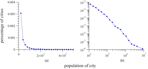
A classic example of this type of distribution is the size of towns and cities [76]. Figure 2.1 plots the histogram of the size of cities. In figure (a) is showed a simple histogram of the distribution of US city sizes. The histogram is highly right-skewed, meaning that while the bulk of the distribution occurs for fairly small sizes—most US cities have small populations—there is a small number of cities with population much higher than the typical value, producing the long tail to the right of the histogram. Figure 2.1 (b) shows the histogram of city sizes again, but this time replotted using a logarithmic scale in the horizontal and vertical axes. As can be observed, a remarkable pattern emerges: the histogram follows a straight line [76, 110].
Figure 2.1. (a) histogram of the populations of all US cities with population
of 10 000 or more. (b) another histogram of the same data, but plotted on logarithmic scales. The approximate straight-line form of the histogram in the right panel implies that the distribution follows a heavy-tailed. Data from the 2000 US Census. Figure and caption originally used by Newman et al. [76]
16 Chapter 2. Background
p(X =x) α Kx(−α) (1)
whereα is a constant parameter of the distribution known as the exponent or scaling
parameter. The scaling parameter typically lies in the range2< α <3, although there are exceptions. In practice, few empirical phenomena obey power laws for all values of
x. More often the power law applies only for values greater than some minimum xmin. In such cases, we state that the tail of the distribution follows a power law.
Another examples of heavy-tailed distributions are Pareto, Lognormal, Exponen-cial, Caughy, and Weibull etc. [13, 35, 37, 76, 104]. There are several approaches to check whether a population follow a heavy-tailed distribution, which we highlight four:
1. Histogram and doubly logarithmic plot: This is a visual approach and it
is most often used. This approach consists in plotting a histogram, applying linear regression, and taking the logarithm of both sides of Equation 1. We can see that the distribution obeys ln(p(x)) = K−α ln(x), implying that it follows a straight line on a doubly logarithmic plot. A common way to check for power-law behavior, therefore, is to measure a variable of interest x, construct a histogram representing its frequency distribution, and plotting that histogram on doubly logarithmic axes. If we discover a distribution that approximately falls on a straight line, we can say that the distribution follows a heavy-tailed, with a scaling parameterαgiven by the absolute slope of the straight line. Typically, this
slope is extracted by performing a least-square linear regression on the logarithm of the histogram. Although this approach is frequently described in the literature, it is subjected to systematic errors under relatively common conditions, and as a consequence the results it provides might not be reliable [24, 103].
2. Statistical approach proposed by Clauset et al. [24]: this approach is a
statistical framework for discerning and quantifying heavy-tailed behavior in em-pirical data. It combines maximum-likelihood fitting methods with goodness-of-fit tests based on the Kolmogorov-Smirnov statistic and likelihood ratios. It also uses numeric methods to estimate the parameters Xmin and α, where Xmin indi-cates the start of the tail and α represents the scaling parameter of the dataset.
Next, the approach calculates the goodness-of-fit between the data and the power law. If the resulting p-value is greater than 0.1 the heavy-tailed is a plausible hypothesis for the data, otherwise it is rejected.
3. Quantile Function: this approach examines a distribution of values and plots
2.3. Statistical Properties of Source Code Metrics 17
dependent variable) as a function of the percentage of observations (independent variable). Also, by using the percentage of observations instead of the frequency, the scale becomes independent of the size of the system making it possible to compare different distributions. Moreover, the quantile function allows for better visualization of the full metric distribution. Therefore, in this PhD thesis all dis-tributions are depicted with quantile plots. Alveset al.also use this approach [5].
4. Adherence test: This approach is also frequently mentioned in the
litera-ture [13, 35]. It relies on rigorous best-fits to several distributions, and checks first whether it is reasonable to fit a heavy-tailed, second whether a given distri-bution is more reasonable than the others, third whether the data can be divided into two or more groups according to which distribution fits “best”.
2.3.1
Metrics Values Distributions
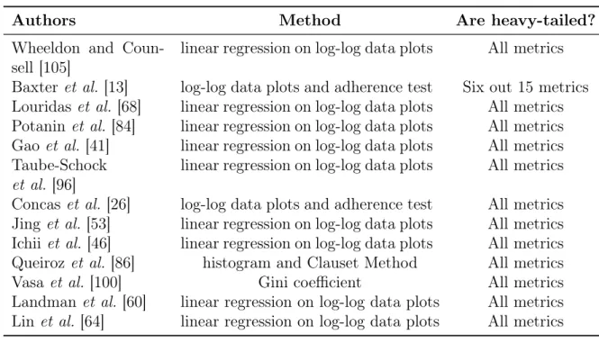
Wheeldon and Counsell analyzed three Java systems: JDK (Java Development Kit), Apache Ant, and Tomcat using 12 metrics related to object-oriented coupling, namely, inheritance, aggregation, interface, parameter type and return type [105]. These met-rics are: Number of methods(nM), Number of fields(nF), Number of constructors(nC), Subclasses (SP), Implemented interfaces (IC), Interface implementations (IP), Refer-ences to class as a member (AP), Members of class type (AC), ReferRefer-ences to class as a parameter (PP), Parameter-type class references (PC), and References to class as return type (RP). To identify the power laws the authors perform linear regres-sion on log-log data plots. They concluded that all metric values follow Power Law distributions.
Baxter et al. analyzed 17 metrics in 56 Java systems for verifying their internal structure [13]. The authors performed adherence tests to identify three types of distri-bution: Power Laws, Lognormal, and Exponential. The goal of this work is to extend the work proposed by Wheeldon and Counsell [105] in order to check heavy-tailed distribution in 17 object-oriented metrics. However, they added the following met-rics: Methods returning classes (RC), Depends on (DO), Depends on inverse (DOinv), Public method count (PubMC), Package size (PkgSize), and Method size (MS). The authors report that, AP, PP, RP, SP, IC, and MS are metrics that follow heavy-tailed distributions. But AC, PC, RC, PubMC, nF, nM, Do, IP, and DoInv do not follow such distributions. Finally, the results for nC and Ms are not conclusive.
18 Chapter 2. Background
heavy-tailed distributions, independently of programming language. These findings are different than those of Baxteret al., which suggests that out-degree metrics are not heavy-tailed [13]. Studies conducted by Potaninet al.[84], Gao et al.[41], and Taube-shock et al. [96] confirm such results for coupling metrics. Potanin et al. analyzed 35 systems and they concluded that coupling metrics are in conformity with heavy-tailed distributions [84]. Gao et al. analyzed four open source Java systems and they also concluded that out-degree and in-degree metrics are in conformity with heavy-tailed distributions [41]. Taube-shock et al. analyzed coupling metrics using 97 open source Java systems from the Qualitas Corpus [96]. The goal of this work was checking the following hypothesis: (i) the between-module connectivity network of source code entities follows a heavy-tailed distribution; and (ii) The between-module connectivity network of source code entities follows a heavy-tailed distribution, and the degree of left skewness has some maximum level. The authors concluded that these two hypothesis can be accepted and that high coupling is impracticable to eliminate entirely from software design.
Concaset al.examined 10 source code metrics of three systems: one implemented in Smalltalk (VisualWorks) and two implemented in Java (JDK e Eclipse) [26]. The goal of this work was to check whether large object-oriented systems follow heavy-tailed distributions. Jing et al. found heavy-tailed in the values of Weighted Methods per Class (WMC) and Coupling Between Objects (CBO) for four open source software systems [53]. Ichii et al. examined four source code metrics on six systems, finding that in-degree follows a Power Law while out-degree follows other heavy-tailed distri-bution [46].
Queirozet al.analyzed the scattering degree of #ifdefsin five
2.4. Thresholds Definitions 19
2.3.2
Discussion
In this section, we provided a discussion about source code metrics distributions, which is summarized in Tables 2.1 and 2.2. We reported that source code metrics tend to follow a heavy-tailed distribution. This means that, typically, software systems follow this pattern: few software entities contain much of the complexity and functionality, whereas the others define simple data abstractions and utilities [101]. Moreover, since non-Gaussian distributions are common in the case of source code metric values de-scriptive statistics, e.g., mean and variance, are not adequated to define thresholds for such metric data. Although, the works reported in this section have theorical value, they fall short in concluding how to use these distributions and their coefficients in practical terms, to establish baseline values to judge systems. Therefore, the next section presents methods to derive source code metric thresholds.
Table 2.1. Source code metric distributions
Authors # Systems Language
Wheeldon and Counsell [105] 3 Java
Baxter et al. [13] 56 Java
Louridas et al. [68] 11 C, Perl, Ruby, and Java
Potanin et al. [84] 35 Java
Gao et al.[41] 4 Java
Taube-Schock et al.[96] 97 Java
Concas et al. [26] 3 Java and Smalltalk
Jing et al.[53] 4 Java
Ichii et al. [46] 4 Java
Queiroz et al. [86] 5 C
Vasa et al. [100] 47 Java and C#
Landman et al.[60] 13K Java
Lin et al. [64] 4 Java
2.4
Thresholds Definitions
20 Chapter 2. Background
Table 2.2. Source code metric distributions
Authors Method Are heavy-tailed?
Wheeldon and Coun-sell [105]
linear regression on log-log data plots All metrics
Baxter et al. [13] log-log data plots and adherence test Six out 15 metrics Louridas et al. [68] linear regression on log-log data plots All metrics Potanin et al.[84] linear regression on log-log data plots All metrics Gao et al.[41] linear regression on log-log data plots All metrics Taube-Schock
et al. [96]
linear regression on log-log data plots All metrics
Concas et al. [26] log-log data plots and adherence test All metrics Jing et al. [53] linear regression on log-log data plots All metrics Ichii et al. [46] linear regression on log-log data plots All metrics Queiroz et al. [86] histogram and Clauset Method All metrics Vasa et al.[100] Gini coefficient All metrics Landman et al. [60] linear regression on log-log data plots All metrics Lin et al. [64] linear regression on log-log data plots All metrics
2.4.1
Extracting Thresholds using Traditional Techniques
Erni and Lewerentz proposed the use of mean (µ) and standard deviation (σ) to derive a thresholdT from project data [32]. For this, the authors used coupling, complexity, and
cohesion metrics. A thresholdT is calculated asTlow =µ+σorThigh =µ−σ, indicating
that high or low values of a metric can cause problems, respectively. This method is a common statistical technique which data are normally distributed. However, the authors did not analyze the underlying distribution, and only applied it to one system, using three releases. Lanza and Marinescu also proposed a method based on descriptive statistics and experts experience [61]. They performed an experiment using source code metrics related to inheritance, coupling, size, and complexity. For this, the authors used 82 systems developed in C++ (37 systems) and Java (45 systems). This method consisted of a intervals of thresholds, where the mean as typical value and standard deviation as upper limit.
2.4. Thresholds Definitions 21
2.4.2
Extracting Thresholds from Repositories
Alves et al. proposed an empirical method to derive threshold values for source code metrics from a benchmark of systems [5]. Their ultimate goal was to use the extract thresholds to build a maintainability assessment model [8, 27, 42]. Specifically, the goal was to define quality profiles to rank entities according to four categories: low risk (0 to 70th percentiles), moderate risk (70th to 80th percentiles), high risk (80th to 90th percentiles), and very-high risk (90th percentile). For this purpose, metric values for a given program entity are first weighted according to the size of the entities in terms of lines of code (SLOC), in order to generate a new distribution where variations in the metrics values are more clear. They illustrated the method using as example the McCabe complexity metric [72] and a benchmark of 100 object-oriented systems, which it was implemented in C# (18 systems) and Java (82 systems), including both proprietary (77 systems) and open source (23 systems). The method of Alves et al. is summarized in six steps [5]:
1. Metrics extraction: the value of the metrics are extracted from a benchmark of systems. For each system S and for each entity E (e.g., method or class), they record a metric value and weight metric. They considered as weight the SLOC of the entity. As example, for the Vuze system, there is a method (entity) called MyTorrentsView.createTabs() with a McCabe value of 17 and
weight value of 119 SLOC;
2. Weight ratio calculation: in this step, for each entity E, they divide the en-tity weight by the sum of all weights of the same system. For each sys-tem, the sum of all entities WeightRatio must be 100%. As example, for the
MyTorrentsView.createTabs() method entity, the result is 119 SLOC
di-vided by 329,765 (total SLOC for Vuze) which represents 0.036% of the overall Vuze system;
3. Entity aggregation: they aggregate the weights of all entities per metric value, which is equivalent to computing a weighted histogram. As example, all entities with a McCabe value of 17 represent 1.458% of the overall SLOC of the Vuze system;
22 Chapter 2. Background
5. Weight ratio aggregation: in this step, a density function (or quantile function) is computed, in which the x-axis represents the weight ratio (0-100%), and the y-axis the metric scale. As example, in the benchmark they used, for 60% of the overall code the maximal McCabe value is 2.
6. Thresholds derivation: thresholds are extracted by choosing the percentage of the overall code we want to represent. For example, for McCabe metric the extracted thresholds are 6, 8 and 14, which represents 70%, 80%, and 90% quantiles.
The authors claimed that the distribution of the metric values is preserved and that the method is resilient to the influence of large systems or outliers. Thresholds were derived using 70%, 80% and 90% quantiles and checked against the benchmark to show that thresholds indeed represent these quantiles. This method was replicated using four other metrics from the SIG quality model: unit size, unit interfacing, FAN-IN, and module interface size. The method also was used by Luijten et al. to derive thresholds to other metrics of the SIG group [69]. Luijten et al.also found empirical evidence that systems with higher technical quality have higher issue solving efficiency. In a more recent work, Alves et al. improved their method to include the calibration of mappings from code-level measurements to system-level ratings, using an N-point rating system [4].
Ferreira et al. defined thresholds for six source code metrics from a benchmark with 40 open source Java systems. The analyzed metrics included coupling factor (COF), number of public fields (NPF), number of public methods (NPM), lack of co-hesion in methods (LCOM), depth of inheritance tree (DIT), and afferent couplings (AC) [35]. The authors used EasyFit tool5
to fit the data to various probability distribu-tions, such as Bernoulli, Binomial, Uniform, Geometric, Hypergeometric, Logarithmic, Binomial, Poisson, Normal, t-Student, Chi-square, Exponential, Lognormal, Pareto, and Weibull. For each metric, the data was collected and two graphics were gener-ated: a scatter plot and the same data in doubly logarithmic scale. Using the EasyFit tool, they concluded that the metric values, with exception of DIT, follow heavy-tailed distributions. After this conclusion, the authors established three threshold ranks: (i) good: refers to most common values; (ii) regular: refers to values with low frequency, but that are not irrelevant; and (iii) bad: refers to values with rare occurrences. How-ever, they do not predefined the percentage of classes tolerated in these categories. For example, the LCOM threshold is: 0 (good cohesion), 1—20 (regular cohesion), and greater than 20 (bad cohesion).
5
2.4. Thresholds Definitions 23
The authors extracted general thresholds for object-oriented software metrics, and thresholds by application domain, size, and system type (tool, library, and frame-work). They did not find relevant differences among them. The identified thresholds were evaluated in two case studies. The results of this evaluation indicated that the proposed thresholds can help to identify classes that violate design principles. Recently, Filo et al.extended and improved this work and they applied it to extract thresholds to 17 source code metrics using a benchmark with 111 open source Java systems [36].
The goal of the methods proposed by Alves et al. [5] and Ferreira et al. [35] is to rank entities, i.e., classes or methods. In the work of Alves et al., a new method was proposed—the use of weighting by size using SLOC metric. The goal of weighing by SLOC is to emphasize the metric variability when plotting the quantile function. Ferreira et al. extracted three thresholds for each metric, which are used to rank the classes as good, regular, or bad. In summary, this works extracted absolute thresholds, meaning that all classes with high value metric are considered as presenting high risk or bad quality. However, several works showed that source code metrics follow a heavy-tailed distribution. Consequently, in this type of distribution is natural to find entities with high values.
2.4.3
Extracting Thresholds using Error Models
24 Chapter 2. Background
succeed in deriving monotonic thresholds,i.e., lower thresholds were derived for higher error categories than for lower ones.
Benlarbiet al.analyzed the relation of source code metric thresholds and software failures using linear regressions [14]. This study was performed using five CK metrics (WMC, DIT, NOC, CBO, and RFC) and two C++ systems. The authors compared two error probability models, one with threshold and another without. For the model with threshold, zero probability of error exists for metric values below the threshold. They concluded that there was no empirical evidence supporting the model with threshold as there was no significant difference among the models. However, this result is only valid for this specific error prediction model and for the metrics the authors took into account. Other models can, potentially, give different results.
Herbold et al. used a machine learning algorithm to define a method for the calculation of metric thresholds [44]. For this, they analyzed 11 metrics related to size, coupling, complexity, and inheritance. In this work, an entity is analyzed according to a set of metrics and the global result is binary. This method is based on a given metric setM and a set of software entitiesX with known classifications Y. As result, the algorithm yields pairs of upper and lower bounds. Specifically, the thresholdsT is
zero (bad) when at least one metric mexceeds its threshold t, and is one (good) when
none of the metrics exceeds its threshold. The authors performed four case studies using eight systems including C functions, C++, C# methods, and Java classes. The results showed that this method is able to improve the efficiency of existing metric sets. The proposed method, however, produces a binary classification and can therefore only differentiate between good and bad; further shades of gray are not possible. Another point is that the extracted thresholds are in entities level. Therefore, system level thresholds are not provided.
2.4.4
Extracting Thresholds using Clustering Algorithms
2.4. Thresholds Definitions 25
However, K-means suffers from important shortcomings: it requires an input parameter that affects both the performance and the accuracy of the results. Thus, different thresholds can be extracted for the same dataset and metric.
2.4.5
Discussion
In this section, we provided a discussion about threshold extraction methods, which are summarized in Table 2.3 and 2.4. We observed that there are several methods for this purpose. However, there is not a method that is widely recognized by researchers and software engineers as an effective instrument to control the internal quality of software systems. We also observed that using benchmark of systems is an interesting approach, which tends to reflect the software development practice.
Table 2.3. Thresholds approaches
Authors Systems Languages Metrics
Erni and Lewer-entz [32]
1 Smaltalk Complexity, coupling, and cohe-sion
Lanza and Mari-nescu [61]
82 C++
and Java
Inheritance, coupling, size, and complexity
Alves et al. [5] 100 C#
and Java
McCabe complexity, unit size, unit interfacing, module interface size, and FAN-IN
Ferreira et al. [35] 40 Java LCOM, DIT, COF, Afferent cou-pling, NOMP, and NOAP
Shatnawi et al. [93] 1 Java CBO, RFC, WMC, LCOM,
DIT, NOC, CTA, CTM, NOAM, NOOM, NOA, and NOO
Catal et al. [20] 5 C and
C++
SLOC, MCave, EC, DC
Benlarbi et al. [14] 2 C++ WMC, DIT, NOC, CBO, and
RFC
Herbold et al. [44] 8 C,
C++, C# and Java
Size, coupling, complexity, and inheritance
Oliveira et al. [83] 86 Java Size metrics
26 Chapter 2. Background
Table 2.4. Thresholds approaches
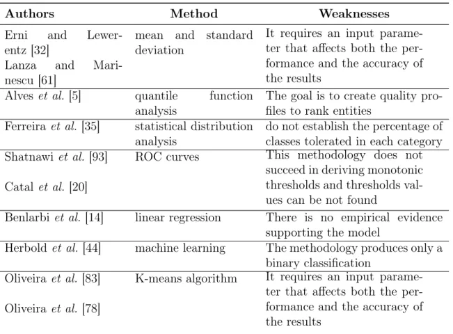
Authors Method Weaknesses
Erni and Lewer-entz [32]
mean and standard deviation
It requires an input parame-ter that affects both the per-formance and the accuracy of the results
Lanza and Mari-nescu [61]
Alveset al. [5] quantile function analysis
The goal is to create quality pro-files to rank entities
Ferreiraet al. [35] statistical distribution analysis
do not establish the percentage of classes tolerated in each category Shatnawiet al. [93] ROC curves This methodology does not
succeed in deriving monotonic thresholds and thresholds val-ues can be not found
Catalet al. [20]
Benlarbiet al. [14] linear regression There is no empirical evidence supporting the model
Herbold et al. [44] machine learning The methodology produces only a binary classification
Oliveira et al. [83] K-means algorithm It requires an input parame-ter that affects both the per-formance and the accuracy of the results
Oliveira et al. [78]
2.5
Studies with Developers
2.6. Final Remarks 27
involved 80 developers with different levels of experience and academic degree. They found that most of the developers are familiar with cohesion and that developers per-ceive cohesion as a measure of a class responsibilities. Moreover, the results showed that conceptual cohesion metrics capture the developers notion of cohesion better than traditional structural cohesion metrics. To the best of our knowledge, the study pre-sented in Chapter 5 is the first on interviewing developers on metric thresholds.
2.6
Final Remarks
Measurement is a fundamental part of Software Engineering research and practice [95]. In this context, software metrics refer to measurements that can be applied to check the quality of processes, projects, and software products. Evaluating software quality through metrics allows to define quantitatively the success or failure of a particular at-tribute, identifying the needs of improvement. In this chapter, we provided a discussion about software quality and presented an overview of source code metrics, specifically, we presented the CK metric suite. We discussed the importance of considering the sta-tistical distribution of software metrics in order to extracted credible thresholds. Next, we presented the state-of-the-art in methods to extract thresholds and we performed a critical appraisal of related work. Finally, we presented related work which explore how developers rate different software quality attributes.
Chapter 3
Proposed Method
This chapter presents the method to extract relative thresholds from a set of systems (Section 3.1). An illustrative example of its usage is presented in Section 3.2. Sec-tion 3.3 discuss some aspects and properties of the proposed method. SecSec-tion 3.4 presents RTTool, an open source tool that automates our method.
3.1
Relative Thresholds
Software metrics have been proposed to analyze and evaluate software by quantitatively capturing a specific characteristic or view of a software system. Despite much research, the practical application of software metrics remains challenging.
We focus on source code metrics that follow heavy-tailed distributions, when measured at the level of classes as long as low(er) metric values are considered to be more desirable than the high(er) ones. Numerous metrics including NOA, NOM, FAN-OUT, RFC, and WMC satisfy these conditions [81, 91, 105]. Examples of a metric that does not follow the traditional heavy-tailed distribution and therefore should not be subject to our method are DIT (Depth of Inheritance) [35] and Dn [90].
Our goal is to derive relative thresholds, i.e., pairs [p, k]such that at least p%of the classes should have M ≤ k, where M is a given source code metric and p is the minimal percentage of classes in each system that should respect the upper limit k. A relative threshold tolerates, therefore, (100−p)% of classes with M > k.
We derive the values of pand k from a curated set of systems, which we call our Corpus. Figure 3.1 defines the functions used to calculate the parameters p and k for a given metric M. First, the function ComplianceRate [p, k] returns the percentage of systems in the Corpus that follows the relative threshold defined by the pair [p, k]. The function ComplianceRatecan be easily increased by increasing k or decreasing p.
30 Chapter 3. Proposed Method
Therefore, ComplianceRate on its own is not sufficient to optimize p and k. Hence, we introduce the notion of a penalty to find the values of p and k. We penalize a ComplianceRatefunction in two situations:
• A ComplianceRate [p, k] less than 90% receives a penalty proportional to its distance to this percentile, as defined by function penalty1[p, k]. As mentioned,
the proposed thresholds should reflect real design rules that are widely common in the Corpus. Therefore, this penalty formalizes this guideline, by fostering the selection of thresholds followed by at least 90% of the systems in the Corpus. In other words, this penalty punishes systems that are somehow “atypical” in the Corpus.
• A ComplianceRate [p, k]receives the second penalty proportional to the distance between k and the median of the 90-th percentiles, of the values of M in each
system in the Corpus, denoted as Median90, as defined by function penalty2[k].
We assume that Median90 is an idealized upper value for M, i.e., a value representing classes that, although present in most systems, have very high values of M1
.
Figure 3.1. ComplianceRate and ComplianceRatePenaltyfunctions
As defined in Figure 3.1, the final penalty of a given threshold is the sum of penalty1[p, k] and penalty2[k], as defined by function ComplianceRatePenalty. Finally,
1
3.2. Illustrative Example 31
the relative threshold is the one with the lowestComplianceRateP enalty[p, k]. In case of ties, we defined a tiebreaker criterion: we select the result with the highest p and then the one with the lowest k.
3.2
Illustrative Example
To illustrate our method we derive a threshold for the Number of Attributes (NOA) metric, based on the systems in the Qualitas Corpus [97]. Figure 3.2 plots the values of the ComplianceRate function, for different values of p and k. As expected, for a
fixed value of p ComplianceRate is a monotonically increasing function, on the val-ues of k. Moreover, as we increase p the function starts to present a slower growth.
This figure 3.2 shows the importance of penalty2. For example, we can observe that ComplianceRate [85,17] = 100%,i.e., in 100% of the systems at least 85% of the classes have NOA ≤ 17. In this case Median90 = 9, i.e., the median of the 90th percentile for the NOA values in the considered Corpusis nine attributes. Therefore, the relative threshold defined by the pair [85,17] relies on a high value for k (k = 17) to achieve a compliance rate of 100%. To penalize a threshold like that, the value of penalty2 is (17−9) /9 = 0.89.Since penalty1 = 0 (due to the 100% of compliance), we have that
ComplianceRatePenalty[85,17] = 0.89.
● ● ● ● ● ● ● ● ● ● ● ● ● ● ● ● ● ●
5 10 15
0 20 40 60 80 100 k Compliance Rate ● ● ● ● ● ● ● ● ● ● ● ● ● ● ● ● ● ● ● ● ● ● ● ● ● ● ● ● ● ● ● ● ● ● ● ● ● ● ● ● ● ● ● ● ● ● ● ● ● ● ● ● ● ● ● ● ● ● ● ● ● ● ● ● ● ● ● ● ● ● ● ● p 75% 80% 85% 90% 95%