www.hydrol-earth-syst-sci.net/18/2265/2014/ doi:10.5194/hess-18-2265-2014
© Author(s) 2014. CC Attribution 3.0 License.
Retrospective analysis of a nonforecasted rain-on-snow flood in
the Alps – a matter of model limitations or unpredictable nature?
O. Rössler1, P. Froidevaux2, U. Börst3, R. Rickli4, O. Martius2, and R. Weingartner1
1Oeschger Center for Climate Change Research and Group for Hydrology, Institute of Geography, University of Bern,
Bern, Switzerland
2Oeschger Center for Climate Change Research and Mobiliar Lab for Climate Impact Research and Natural Hazards,
Institute of Geography, University of Bern, Bern, Switzerland
3Department of Geography, University of Bonn, Bonn, Germany 4BKW FMB Energy AG, Bern, Switzerland
Correspondence to:O. Rössler (ole.roessler@giub.unibe.ch)
Received: 20 September 2013 – Published in Hydrol. Earth Syst. Sci. Discuss.: 29 October 2013 Revised: 13 March 2014 – Accepted: 26 March 2014 – Published: 19 June 2014
Abstract. A rain-on-snow flood occurred in the Bernese Alps, Switzerland, on 10 October 2011, and caused signifi-cant damage. As the flood peak was unpredicted by the flood forecast system, questions were raised concerning the causes and the predictability of the event. Here, we aimed to recon-struct the anatomy of this rain-on-snow flood in the Lötschen Valley (160 km2) by analyzing meteorological data from the synoptic to the local scale and by reproducing the flood peak with the hydrological model WaSiM-ETH (Water Flow and Balance Simulation Model). This in order to gain process un-derstanding and to evaluate the predictability.
The atmospheric drivers of this rain-on-snow flood were (i) sustained snowfall followed by (ii) the passage of an atmo-spheric river bringing warm and moist air towards the Alps. As a result, intensive rainfall (average of 100 mm day−1) was
accompanied by a temperature increase that shifted the 0◦ line from 1500 to 3200 m a.s.l. (meters above sea level) in 24 h with a maximum increase of 9 K in 9 h. The south-facing slope of the valley received significantly more precipitation than the north-facing slope, leading to flooding only in tribu-taries along the south-facing slope. We hypothesized that the reason for this very local rainfall distribution was a cavity circulation combined with a seeder-feeder-cloud system en-hancing local rainfall and snowmelt along the south-facing slope.
By applying and considerably recalibrating the standard hydrological model setup, we proved that both latent and sen-sible heat fluxes were needed to reconstruct the snow cover dynamic, and that locally high-precipitation sums (160 mm in 12 h) were required to produce the estimated flood peak.
However, to reproduce the rapid runoff responses during the event, we conceptually represent likely lateral flow dynamics within the snow cover causing the model to react “oversensi-tively” to meltwater.
Driving the optimized model with COSMO (Consortium for Small-scale Modeling)-2 forecast data, we still failed to simulate the flood because COSMO-2 forecast data underes-timated both the local precipitation peak and the temperature increase. Thus we conclude that this rain-on-snow flood was, in general, predictable, but requires a special hydrological model setup and extensive and locally precise meteorological input data. Although, this data quality may not be achieved with forecast data, an additional model with a specific rain-on-snow configuration can provide useful information when rain-on-snow events are likely to occur.
1 Introduction
buried for several hundred meters, and the underlying water reservoir was filled with 200 000 m3of debris. Fortunately, there were no injuries, but the flood caused total damages of approximately CHF 90 million (Andres et al., 2012).
Flood predictions using coupled numerical weather pre-dictions (NWP) and deterministic hydrological models are today a standard approach that is further extended using ensemble forecast systems (EPS) to cope with model un-certainties (see review of Cloke and Pappenberger, 2009). In Switzerland, this approach is implemented by combin-ing COSMO (Consortium for Small-scale Modelcombin-ing) and COSMO-LEPS (COSMO- Limited-area Ensemble Predic-tion System) forecast data with an extended HBV (Hydrol-ogiska Byråns Vattenbalansavdelning) hydrological model (FOEN, 2009). A dense network of discharge gauging sta-tions is maintained, and the Federal Office for the Environ-ment (FOEN) operationally forecasts the discharge of sev-eral river systems. In fact, rising water levels for the river Kander (Bernese Oberland) were predicted for this flood, but the peak on 11 October 2011 was strongly underestimated – below the warning level.
Shortly after this extreme event, the following questions were raised: (a) what exactly caused the flood? and (b) why was this event not properly forecasted to warn the public? The authority in charge of hydrological warnings, the FOEN commissioned a study to analyze the causes of this flood event. The present study is based on a contribution to the FOEN study (Rössler et al., 2013).
The flood was preceded by a special weather situation: during the first week of October 2011, a strong high-pressure system brought a period of warm and clear weather to the Swiss Alps. These stable weather conditions were replaced by an extratropical cyclone on 7 October that led to extensive snowfall down to 1200 m a.s.l.(abovesealevel).The snowfall lasted until 9 October. After some hours of sunshine on 9 Oc-tober, a warm front reached the Alps from the northwest in the early morning of 10 October and triggered heavy rainfall locally. The flood was hence a typical rain-on-snow event.
Rain-on-snow floods are known as one of five flood types occurring in temperate climate mountain river systems (Merz and Blöschl, 2003). While most studies about rain-on-snow events have been done in North America (e.g., Kattelmann, 1997; Marks et al., 1998; McCabe et al., 2007), this flood type is also reported in Europe (e.g., Sui and Koehler, 2001), Japan (Whitaker and Sugiyama, 2005), and New Zealand (Conway, 2004). The entering rainfall water is generally irregularly distributed in the snowpack, forming saturated zones, vertical flow fingers and lateral flow forms (Kattel-mann and Dozier, 1998). Kattel(Kattel-mann and Dozier (1998) also stated that the idea of a uniform wetting front is inappro-priate. Eiriksson et al. (2013) showed that especially during rain-on-snow events significant volumes of fast lateral flows contributed to the total runoff amplifying the water responses from soils. Although these highly dynamic processes have been described since decades (e.g., Wankiewicz, 1978),
cur-rent state-of-the-art hydrological models represent these pro-cesses in a much more static manner: snow is regarded as a 1-D (one-dimensional) single-linear storage with a defined water holding capacity that releases water to the soil surface for infiltration. Lateral processes in the snow cover are not considered.
According to McCabe et al. (2007), the main driving fac-tors for a rain-on-snow flood are the extent of the snow-covered area, the freezing and thawing elevations, the wa-ter equivalent of the snow cover, and the liquid precipitation amount. Merz and Blöschl (2003) also stress the importance of latent heat input and point to the occurrence of overland flow during rain-on-snow events because soils are saturated by antecedent snowmelt processes. In the present case, soils were certainly not saturated as indicated by the dry pre-event conditions and the continuous freezing temperature level dur-ing the snow accumulation period. Interestdur-ingly, the rapid runoff responses observed still point to the occurrence of sur-face flow.
In general, the prediction of floods remains challeng-ing as small differences in precipitation and temperature cause strong biases in the hydrological prediction, especially in mountainous areas with small response times, and the sensitive effect of the snow limit determination on runoff (Jasper et al., 2002). The prediction of rain-on-snow events is even more challenging as it requires accurate informa-tion on snow-covered area and snow water equivalent. Mc-Cabe et al. (2007) stated that the prediction of rain-on-snow events is not only limited by the meteorological input pa-rameter, but also by insufficient knowledge about the impor-tant processes involved. The latter is even more valid for Eu-rope with far less research attention on rain-on-snow events, than for instance in North America. Hence, data of observed rain-on-snow events and case studies revealing in detail the causes and process sequences of this important and fascinat-ing hydro-meteorological process is required to improve our process understanding and to improve the forecastability of such extreme events.
predictability of the rain-on-snow flood by driving the hydro-logical model with COSMO-2 forecast data. This will lead to a final assessment of past and future predictability of such rain-on-snow events.
2 Materials and methods 2.1 Study area
The Lötschen Valley lies just south of the Bernese Alps, which acts as the first barrier for the predomi-nantly northwestern atmospheric inflows. As a result, the highest annual precipitation amounts in Switzerland are found within this mountain range (Jungfrau, Eiger, Mönch,
>3600 mm year−1, Kirchhofer and Sevruk, 2010). The
Lötschen Valley is situated in the transition zone between this area of highest precipitation amounts and the driest re-gion in Switzerland (Rhone Valley, Stalden, 535 mm year−1).
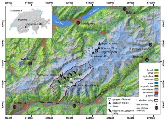
The valley (Fig. 1) stretches from 600 m at the southern out-let up to approximately 4000 m a.s.l., with a mean elevation of 1800 m a.s.l. The valley bottom extends from the south-west to the northeast and rises slightly from approximately 1200 to 2100 m a.s.l. at the glacier tongue; all of the sur-rounding mountain ridges are approximately 3000 m a.s.l., and the mountain tops are higher. Dominant vegetation types are coniferous mountain forests and Alpine pastures. Nearly 18 % of the catchment is glaciated. The Lonza is the main river in the valley and is fed by numerous small tributary rivers from the north- and south-facing slopes and the high-est elevations. The black arrows in Fig. 1 mark the rivers that had extraordinary floods during the October event (from left to right: Ferdenbach, Milibach, Tännbach, and Gisentella). Notably, none of the rivers on the north-facing slope showed any extreme flooding.
2.2 Methods for reconstructing the flood 2.2.1 Reanalysis and soundings data
The 4-day synoptic evolution preceding the event is analyzed using the ERA-Interim (Interim ECMWF Re-Analysis) data set from the European Center for Medium-Range Weather Forecasts (ECMWF) (Dee et al., 2011). This reanalysis data set results from a numerical weather prediction model frozen in time that is continuously forced by a complex assimilation of various observations of the atmosphere, ocean, and land surface. It is commonly used for the retrospective analysis of meteorological situations. The main atmospheric variables are available on a three-dimensional grid (T255 horizontal resolution, interpolated to a 1◦×1◦grid, 90 vertical layers)
every 6 h. In addition to these gridded data, vertical charac-teristics of the atmosphere recorded from weather balloons launched in Payerne (cp. Fig. 1) were analyzed. The Payerne upper-air soundings station is located in the Swiss Plateau 80 km northwest of the Lötschen Valley (upstream of the
in-vestigated flood event, see Fig. 1). These weather balloons are launched twice a day and provide high-resolution profiles of temperature, humidity, wind velocity, wind direction and pressure. Here, we compared radio-sounding data from the day before (9 October, 00:00 UTC – Coordinated Universal Time) with data from the day of the flood event (10 October, 00:00 UTC).
2.2.2 Local meteorological observations
The local development of the hydro-meteorological event is analyzed in detail using data from a dense network of obser-vations in the Lötschen Valley. The Lonza River discharge is officially measured by the FOEN at the center of the val-ley (Blatten gauge, Fig. 1), and inflow to the reservoir of the EnAlpin hydropower plant was provided by the operat-ing company for the event period (Ferden reservoir gauge, Fig. 1). Eight meteorological stations are distributed in the valley. These stations are located on both sides of the valley at different elevations. Two stations are operated by the In-stitute for Snow and Avalanche Research (SLF), and one is operated by a private weather service, MeteoMedia. All other stations were set up by the Department of Geography, Uni-versity of Bonn (GIUB) during a previous research project (Börst, 2005, cp. Table 1). This high network density enables a very detailed analysis of the meteorological conditions in the valley during the rain-on-snow event. The meteorological stations are equipped with standard measuring devices for temperature, precipitation, air humidity, wind speed, wind direction, global radiation, and snow depth. Table 1 summa-rizes the location and equipment at each station; IDs refer to the numbers in Fig. 1. All rain gauges are unheated; there-fore, precipitation depth and duration during snowfall and in the transition from snow to rainfall must be analyzed with caution.
2.2.3 Hydrological modeling
Figure 1.Location of the Lötschen Valley in Switzerland and the land cover characteristics of the valley. The black arrows indicate the flooding rivers, red dots and black circles represent meteorological stations and white triangles represent discharge gauges. Recordings from the meteorological stations in the Lötschen Valley will be analyzed in Sect. 3.2. The stations’ names are (1) Ried, (2) Chumme, (3) Grund, (4) Grossi Tola, (5) Mannlich, (6) Sackhorn, (7) Gandegg, and (8) Wiler.
Table 1.Meteorological stations in the catchment with the param-eters measured, the elevation of the location, and the supporting institution.
ID
cp.
Fig.
1
Meteorological station Institution Ele
v
ation,
m
a.s.l.
T
emperature Precipitation Snow
height
W
ind
speed
W
ind
direction
Relati
v
e
humidity
1 Ried GIUB 1470 × × × × × ×
2 Chumme GIUB 2210 × × × × × ×
3 Grund GIUB 1855 × × × × × ×
4 Grossi Tola GIUB 2880 × × – × × ×
5 Mannlich GIUB 2250 × × × × × ×
6 Sackhorn SLF 3200 × – – × × ×
7 Gandegg SLF 2717 × × × × × ×
8 Wiler MeteoMedia 1415 × × – × × ×
are superposed for runoff generation, and runoff concentra-tion is described by conceptual recession parameters that re-fer to the response time of a catchment after rainfall. These recession constants are used for direct runoff (kd) and
in-terflow (ki) and need to be derived from the hydrograph or
need to be calibrated (Hölzel et al., 2011). WaSiM-ETH re-quires spatial data of soil and land use types and a digital elevation model. The characteristics of the two former data sets must be parameterized according to the assigned types
(e.g., soil hydraulic properties, soil magnitude, root depth, and leaf area index). Meteorological information for each raster cell is generated by interpolating meteorological point data to the entire catchment, which can be achieved in sev-eral ways. The simplest methods are the Thiessen polygon interpolation and the inverse distance weighting (hereafter IDW) methods; these methods depend solely on the spa-tial distribution of the meteorological stations. A more ad-vanced method is the combination of IDW with an elevation-dependent regression (IDWREG). Elevation-elevation-dependent re-gression can be useful in areas with high elevation gradi-ents, such as the Lötschen Valley. In addition, WaSiM-ETH is able to make use of externally processed data, such as the COSMO forecast data sets. All of these methods are described in more detail by Schulla (2013). As the focus of this study is the simulation of a rain-on-snow event, the reproduction of snowmelt is crucial. In WaSiM-ETH, dif-ferent methods can be applied. The standard technique is a degree-day-factor model (hereafter called SM1) that sim-ply multiplies a degree-day factor (C0) with the temperature
above the temperature of snowmelt (T0). In addition,
WaSiM-ETH offers the possibility to consider latent heat fluxes as they occur during rain-on-snow events using an energy bal-ance model after Anderson (1973) (hereafter called SM2). For precipitation sums of more than 2 mm day−1, the SM2
heat (degree-day factors (C1, C2) considering wind speed,
(C1+C2·windspeed)·snowmelt temperature), latent heat considering saturation deficit
(C1+C2·windspeed)·(saturation vapro pressure−
6.11)·psychrometric constant−1, radiation melt
(1.2·air temperature), and energy from liquid
precipi-tation (0.0125·precipitation·air temperature) (cp. Schulla, 2013). The factor in the latter equation represents the heat transfer of rainfall water into the snow and is the specific heat of water (4.184 J g−1K−1) divided by melting energy of
snow (333.5 J g−1). When the precipitation amount during
one time step is less than 2 mm, melt is calculated using the simple degree-day-factor model (SM1). In addition, the SM2 also subdivides the snow cover into a liquid and a solid part and the maximum water holding capacity has to be parameterized (standard 10 %, Schulla, 2013). In both model versions the water from snowmelt and rainfall percolates without delay through the snow cover and infiltrates into the soil. To account for lateral processes in the snow cover, a fraction of this water is directly attributed to surface runoff (parameterSF). This fraction needs to be calibrated.
To analyze the key processes causing the flood, we ap-plied a previously calibrated model version (Rössler and Löf-fler, 2010) in a recent version of WaSiM-ETH (version 9.2, Schulla, 2013). The model has a temporal resolution of 1 h and a spatial resolution of 50 m×50 m. It was calibrated (cal.) against discharge for the year 2002 and validated (val.) for the 2003–2007 period. Statistical measures such as the Nash– Sutcliffe index (cal.: 0.84, val.: 0.8), Pearson’sr(cal.: 0.94, val.: 0.95) and the index of agreement (cal.: 0.96, val.: 0.95), in addition to the water balance, demonstrated the model’s ability to reproduce discharge from the Lonza catchment (Rössler and Löffler, 2010).
2.2.4 Stepwise recalibration of the standard hydrological model
The hydrological modeling in general should not be stood as an end in itself but as a tool to improve the under-standing of the process and the forecast. The former is espe-cially the case if models are not consistent with the obser-vations (Beven, 2001). Applying a previously calibrated hy-drology to the flood event, we found that the model strongly underestimated the event. Thus, we assumed that recalibrat-ing this model to fit the observations will indicate the rel-evant flood-generating processes. As this event was a one-time flood, the classical calibration–validation–verification procedure is inapplicable. Instead, a stepwise recalibration based on hard and soft information of processes was applied following Hölzel et al. (2011). Each recalibration step was underpinned by hypothetical assumptions of the underlying processes. These recalibration steps were done consecutively with increasing degree of standard model modifications: first, we changed individual model parameters, then we tried dif-ferent snow-model algorithms, and finally we changed input
data sets to reproduce this rain-on-snow flood event. This ap-proach enabled the evaluation of the extent to which the stan-dard model deviated from this extreme event and indicated the key processes and model configurations leading to this flood. However, the transferability of the recalibrated model to other events or other regions remained unproved.
1. Recalibrating model parameters
In the course of this study, three model parameters (“fraction of direct flow from snowmelt” (SF),
“run-time of direct flow (kd) and interflow (ki)”, and the melt
factors of the snow modules (C0, C1, C2)) were
re-calibrated to account for deviations between the mod-eled and the observed discharge. The “fraction of di-rect flow from snowmelt” (SF, Schulla, 2013) defines
the proportion of liquid water in the snow cover that in-filtrates into the soils and the proportion that is directly assigned to surface runoff. In this study, we increased this value considerably (from 10 to 90 %) under the as-sumption that the snow cover was saturated very quickly and that lateral flow processes were dominant. Although this recalibration was necessary to fit the model to the observed runoff, the increased value is quite high and therefore unlikely, but still possible. For the same rea-sons, we decreased the “response times of direct flow and interflow”, which indicate the response time to pre-cipitation events in the catchment. These parameters are typically derived from a hydrograph if observations are available. These conceptional parameters are also used to increase runoff response time due to lateral water movement in the snow cover.
Finally, melt factors determine the amount of water that is melted per time step and the energy available (latent and sensible). The melt factors were calibrated with respect to both discharge and snow water equiva-lent (SWE) by comparing model output with observed runoff at Lonza (Ferden) and observed snow water equivalent at the SLF station Gandegg (2717 m a.s.l.). Observed SWE is derived from measured snow depth, assuming a snow density of 0.1 g cm−3for newly fallen
snow. Accordingly, derived observed SWE was com-pared only with the modeled solid part of the snow cover. Nevertheless, snow density is very sensitive to the validation of the modeled SWE: according to Judson and Doesken (2000) snow density can range from 0.05 to 0.35 g cm−3; Jonas et al. (2013) assumed for the same
rain-on-snow event a value of 0.15 g cm−3; and an
(0.075–0.125 g cm−3). We avoided applying multiple
variable snow densities during the event, as this would result in wide range of possible SWE and impede the validation of modeled SWE. The modeling of the snow dynamic was validated at all further stations in the Lötschen Valley.
2. Changing the snow module algorithm
We used two of the four different snow modules avail-able in WaSiM-ETH. First, we applied the simple but straightforward empirical temperature degree-day ap-proach (SM1). This apap-proach tries to conceptually de-scribe all melting energy by using only the sensible heat (temperature). Second, a more physically based snowmelt model was used that calculates the melt as the sum of sensible- (temperature) and latent-heat-related melt (SM2). Latent-heat-related melt is calculated from wind speed, air humidity, and radiation. The perfor-mance of these modules indicates whether sensible heat alone or a combination of latent and sensible heat con-trols snowmelt and runoff generation.
3. Refining the input data sets
Precipitation is a crucial input data set; accordingly, the applied regionalization approach and the chosen meteo-rological stations determine the modeling results. Ini-tially, we used the IDWREG approach based on the same official meteorological stations as used in the first calibration and added one additional station (Gandegg, Fig. 1) situated directly within the most affected catch-ment Milibach. Subsequently, we used a refined data set that incorporates all official (see Fig. 1) and all private meteorological stations available (see Table 1), despite their inaccuracies in recording solid versus liquid pre-cipitation. Snowfall measurements from the SLF station Gandegg was found to be more accurate compared to snow measurements from private stations. Hence, we fitted the precipitation against snow depths (assuming a density of 0.1 g cm−3) measured at the SLF IMIS
(Inter-cantonal Measurement and Information System) station Gandegg. This resulted in a correction factor of 0.85 for snowfall. In terms of liquid precipitation an overestima-tion is likely as this measured rainfall is biased by the snow in the rain gauge. Here, we also applied a reduc-tion of 15 % (up to 24 mm). As this procedure is quite uncertain, we evaluated these corrections against dis-charge and snow measurements from all private stations and found the best performance using this correction. All model parameters for the standard model setup as well as the recalibrated values of all model versions used are sum-marized in Table 2.
2.2.5 Test of the event’s predictability
To test the predictability of the event, we applied the opti-mized model that reproduced the flood peak best and used the COSMO-2 forecast model data (Meteoschweiz, 2010) as meteorological input data. COSMO-2 is a high-resolution numerical weather forecast model with a spatial resolution of 2.2 km×2.2 km. It is used by several meteorological ser-vices in Europe; in Switzerland, it is applied in combination with the coarser resolution COSMO-7 model. COSMO-2 is updated eight times a day and provides a forecast of 24 h. Here, we used COSMO-2 temperature and precipitation data from 18, 12, and 6 h in advance of the flood peak on Monday, 10 October 2011, 12:00 UTC.
3 Results
3.1 Precursor weather conditions
The weather conditions in the Lötschen Valley between 7 and 10 October first changed from warm, dry, and bright conditions to cold temperatures and snowfall on 7 October (−14 K from 6 October 11:00 UTC to 7 October 11:00 UTC, ECMWF data), and then changed back to warm conditions with significant amounts of liquid precipitation on 10 Octo-ber (+9 K and more than 100 mm of rain locally, ECMWF data). The following large-scale atmospheric flow evolution was responsible for these rapid changes in temperature and precipitation.
Figure 2.ECMWF reanalysis data on 7 October 2011 00:00 UTC (top row), 8 October 2011 12:00 UTC (middle row), and 10 October 2011 00:00 UTC (bottom row). The left column(a–c)displays temperature in degrees Celsius at 850 hPa (color) together with sea level pressure in hectopascal (contours). The right column(d–f)shows the vertically integrated precipitable water of the atmosphere in millimeters (color) together with the 740 hPa wind in meters per second (arrows). The red line in the right column refers to the potential vorticity (PV) and illustrates the 2 PV unit limit on the 320 K isentrope. Violet lines in(d–f)indicate the outline of atmospheric river conditions, based on the definition by Ralph and Dettinger (2011).
fulfilled the characteristics of an atmospheric river (AR, vi-olet contour line in Fig. 2d–f) as defined by Ralph and Det-tinger (2011). The vertically integrated precipitable water ex-ceeded 20 mm, wind speed in the lowest 2 km was greater than 12.5 m s−1, it was a few hundred kilometers wide and
it extended for thousands of kilometers across the North At-lantic (Fig. 2d–f).
Comparing the event with all October data in the ERA-Interim at the grid point upstream of the Lötschental (47◦N, 7◦E), we found that negative temperatures at 850 hPa oc-curred on approximately 3 days month−1in October during
the 33 years considered. The warm temperature on 10
associated with the passage of a high potential vorticity (PV) trough, or positive PV anomaly, at the tropopause level. The evolution of the tropopause level flow is illustrated using the dynamical tropopause on the 325 K isentropic surface (Fig. 2d–f, red line). The dynamical tropopause is co-located with the jet. Positive upper level PV anomalies influence the structure of the atmosphere underneath them, such that colder air and reduced stability are typically found below (e.g., Schlemmer et al., 2010). The red line in Fig. 2d–f show the subsequent development of the PV anomaly. The excur-sion of polar air towards the Equator is located below the positive PV anomaly and the passing of the cold and warm fronts corresponds to the upstream and downstream flanks of the trough, respectively. A more general statement is that the passage of a trough followed by the passage of a ridge and the associated major variations of upper level PV must co-incide with important changes in stability, vorticity and tem-perature in the mid to low troposphere. Such rapid and in-tense changes of the flow properties over areas as large as the Alpine range must coincide with the meridional transport of air masses and abrupt air mass transitions.
The vertical extent of the change from cold and dry to warm and wet atmospheric conditions was captured by the upper air soundings launched in Payerne at 00:00 UTC on 9 and 10 October (Fig. 3). The comparison of the two profiles shows that the freezing level rose from 1500 to 3000 m a.s.l.
in 24 h. This strong warming was associated with a remark-able moistening as depicted by the concomitant rise of the zero-degree dew point temperature from approximately 1500 to 3000 m a.s.l. In the profile from 10 October, two differ-ent air masses can be distinguished: a very stable (isother-mic) and cold layer extended from the surface up to 800 hPa on top of which a less stable layer extended over the whole tropopause. This points to flow blocking along the northern face of the Alps at the time of the warm front’s arrival. The low-level cold pool might have played a role in determining the distribution of precipitation by prelifting the air and by creating a level of wind shear (between the retarded blocked flow and the fast unblocked flow). Strong shear can favor the development of turbulent cells embedded in a cloud layer and associated up- and downdrafts, which in turn might in-fluence precipitation growth mechanisms significantly (see, e.g., Houze and Medina, 2005). The wind direction (not shown) was mostly NW–N from 2000 m upwards.
That the air was lifted over the Alps rather than being blocked by the Alpine barrier can be determined from the Froude number (F) (Reinecke and Durran, 2008).F is the ratio between the kinetic energy of the wind and the energy required to pass over a barrier. IfF >1, the air can surpass the Alpine barrier. F was >1 from 2200 m upwards (not shown), indicating that the air masses located approximately 2200 m a.s.l.above Payerne were flowing over the Alps, re-sulting in a north foehn condition. Values of F <1 below 2200 m a.s.l.confirm the presence of a blocked cold air pool near the surface.
Figure 3.Skew-t–log-P diagram showing the vertical atmospheric structure as measured from weather balloons launched at Payerne (cf. Fig. 1) on 9 October 2011 00:00 UTC (blue lines) and 10 Oc-tober 2011 00:00 UTC (orange lines). The profile of the Lötschen Valley as retrieved by surface meteorological stations is included for comparison (red for 9 October 00:00 UTC and black for 10 Octo-ber 00:00 UTC). The main ridge of the Lötschen Valley has a mean elevation of approximately 3000 m a.s.l.(thick horizontal line).
It is interesting to compare the temperature profiles re-trieved from the upper air sounding with the 2 m tempera-ture profiles of the Lötschen Valley retrieved from surface thermometers (Fig. 3). While the vertical profiles are very similar on 9 October 00:00 UTC, the valley floor is signif-icantly cooler than the free air on 10 October 00:00 UTC. This difference might be the result of the intense snowmelt during the passage of the warm front. Snowmelt requires sig-nificant energy input from the surface air and evidence for it is given later by station measurements. The soundings them-selves also show that large-scale conditions were very suit-able for widespread and intense snowmelt. Both the tempera-ture and the dew point temperatempera-ture reached positive values up to 3000 m a.s.l.A positive dew point temperature is very im-portant for snowmelt. If air with a positive dew point temper-ature is in contact with snow, and hence cooled to 0◦C, it will be oversaturated and condensation will set in. Each gram of condensed water vapor releases sufficient energy to melt 7 g of snow; therefore, snowmelt will be significantly enhanced by latent heat transfer adding to sensible heat transfer from the air into the snow.
climatology. This situation would have been harmless, how-ever, without an unusually rapid rise of the snow line and the sudden arrival of warm and moist air (AR) from the north-west on the evening of 9 October. The AR resulted in an exceptionally intense transport of moisture towards the Alps and significant amounts of rainfall on 10 October over the freshly snow-covered areas.
3.2 Local meteorological conditions
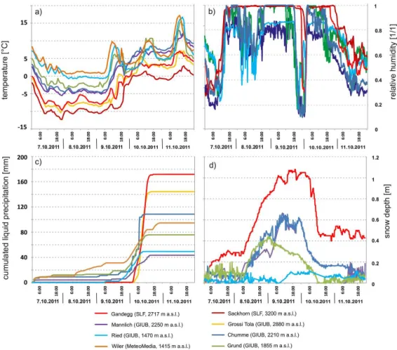
Eight stations distributed throughout the Lötschen Valley confirmed the course of the general weather conditions pre-viously described. Figure 4a–d summarize the development of the 2 m air temperature (Fig. 4a), the relatively humidity (Fig. 4b), the accumulated liquid (Fig. 4c), and the solid pre-cipitation (Fig. 4d) from 7 to 10 October at each station. A strong cooling occurred on 7 October and negative tempera-tures where recorded down to 1470 m a.s.l.(Ried) on 8 Oc-tober and early 9 OcOc-tober, confirming that the snow limit was situated at approximately 1500 m. Only the Wiler sta-tion, at 1415 m, experienced slightly positive temperatures. On 9 October, the stations at the valley bottom recorded a diurnal temperature increase of up to 9 K, which might in-dicate an intermediate period of clear sky. In contrast, no significant diurnal temperature cycle was recorded at higher elevations. Between 9 October in the evening and the morn-ing of 10 October, a rapid warmmorn-ing was recorded at all sta-tions (up to+10 K). The zero-degree line was found around 1500 m a.s.l.(Wiler) before and around 3200 m a.s.l.during the event (Sackhorn). This warming coincided with the ar-rival of the warm front and was most pronounced close to the northern crest, at the Sackhorn and Gandegg stations (cp. Fig. 1).
The temporal evolution of liquid (Fig. 4c) and solid (Fig. 4d) precipitation was similar at all stations, but the recorded precipitation amounts varied significantly. Rainfall amounts generally increased with altitude and, interestingly, significantly more rain fell on the south-facing slope than on the north-facing slope. For example, the Chumme station recorded more than twice as much precipitation (108 mm) than the Mannlich station (42 mm) at the same elevation on the opposite slope. The small-scale wind field that caused this rainfall pattern will be discussed at the end of this sec-tion. The highest precipitation amounts at the valley bottom were found near Wiler; precipitation first decreased going eastward (Ried) before increasing with increasing elevation (comparing Wiler–Ried–Grund–GrossiTola).
Snow depth was more linearly correlated to altitude than rainfall, with snowfall starting earlier, lasting longer and be-ing more intensive at higher elevations. For example, the snow amounts recorded at Chumme and Mannlich are simi-lar. Evidence for snowmelt is given by the rapid decrease of snow depths, amounting to 40 cm at Chumme and Mannlich and 60 cm at Gandegg within 6 h in the morning of 10 Octo-ber. The onset of snowmelt is delayed by several hours
go-ing from 1900 (Grund) to 2200 (Chumme and Mannlich) to 2700 m (Gandegg) because of lower temperatures at higher elevations. Minor snow accumulation is also recorded at Ried (1470 m a.s.l.) with a maximum of 10 cm. A slight ablation is also visible. A more exact estimation of the snow cover dynamic is not possible due to the measurement uncertain-ties. Those uncertainties are expressed in the strong and short fluctuations visible in all snow depth curves and stem from wind drift, movements of the underlying grass, shrinking and swelling of the soil, and freeze–thaw processes.
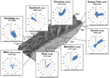
Figure 5 shows wind directions recorded on 10 October at 8 stations inside the Lötschen Valley. The diagrams indicate the numbers of measurements (relative frequency) from each direction. Sackhorn station (located at the valley crest) is the only one recording a high frequency of NW wind consis-tent with the synoptic-scale flow (the wind blew exclusively from a WNW to NW direction). It is the only station directly exposed to the incoming synoptic wind from the NW. All of the other stations, located on northern flank of the val-ley, i.e., the lee side of the northern crest, registered local circulations inside the valley. Ried, Grund, and Grossi Tola stations along the WSW–ENE valley axis recorded along-valley winds with a predominance of wind in the downs-lope direction. At Wiler, the wind direction was highly vari-able. Both mid-slope stations, Chumme and Mannlich, show wind directions similar to those at the valley bottom. Particu-larly interesting is the Gandegg station, which is the only one recording a SE wind. Remarkably, the wind direction at Gan-degg was opposite to the wind direction at Sackhorn, which is located only 1.3 km away.
The synoptic situation was conductive to a rain-on-snow event with the successive passage of two precipitation– producing fronts, a rapid rise of the snow line and excep-tional amounts of moisture transported towards the Alps. In addition to the synoptic forcing, the dense network of me-teorological stations points to strong variations at the local scale. The rain-on-snow event was intense close to the north-ern crest (10 K temperature increase in 12 h, approx. 160 mm in 12 h, and a snow depth decrease of 60 cm in 12 h at Gan-degg) and gradually less intense from north to south across the valley. Rainfall totals decreased by a factor of 4 along a 6 km cross section between Gandegg and Mannlich. This remarkably steep rainfall gradient indicates kilometer-scale heterogeneity of the atmospheric flow.
Figure 4.Temperature(a), relative humidity(b), accumulated liquid precipitation(c), and snow height(d)measured at eight meteorological stations in the Lötschen Valley. The time series describe the overall course of the weather and reveal strongly heterogeneous rainfall amounts.
(see e.g., example Wirth et al., 2012). We have no proof of a cavity circulation early on 10 October, but some evidence points towards its probable occurrence. First, the wind di-rections recorded at Gandegg were upslope, i.e., opposite to the background wind. Second, relative humidity indicated the occurrence of a surface cloud along the upper southward fac-ing slope. Third, the Froude number was much larger than unity, indicating the presence of “flow over” conditions nec-essary for the formation of cavity circulation. A cavity cir-culation implies upslope ascent on the lee side of the moun-tain crest as shown in Fig. 6. Such an upslope ascent and the associated adiabatic cooling, saturation, and cloud for-mation at low levels, can enhance snowmelt very efficiently through sensible and latent heat transfer to the snow. Rain-fall can also be enhanced significantly by low level clouds through the seeder–feeder effect. Indeed, in the case of low-level clouds, the hydrometeors created higher above by the seeder cloud fall through a saturated layer and are not evap-orated. Moreover, they collide with the low-level droplets so that rainfall efficiency can rise significantly. Forced ascent from the topography and saturated air is likely to have pro-duced a low-level cloud on the windward side of the northern crest as well; therefore, intense snowmelt and intense
precipi-tation is likely to have occurred on both sides of the Lötschen Valley’s northern crest. There is unfortunately no measure-ment station on the windward side, but flooding, landslides, and damages have been reported from the Gasteren Valley, which contributed to the 100-year flood event in the Kander Valley.
The rapid decrease of snow depth as measured at the Gan-degg station might be interpreted as either efficient snowmelt accelerated by high surface-water vapor and/or snowpack melt and compaction by locally enhanced rainfall. The rain was most likely stored in the fresh snowpack until saturation was reached. Additionally, the snowpack not only acted as a runoff enhancer by trapping and releasing the rainfall water, but also by contributing a considerable amount of snowmelt water to the runoff.
3.3 Retrospective modeling of the event
Figure 5.Frequency of 2 m wind directions from station measure-ments on 10 October in the Lötschen Valley. The radial component of each direction (in blue) indicates the number of measurements when the wind was blowing from that respective direction in 24 h. Note that the total number of measurements varies since wind is measured every 60, 30 or 10 min depending on the station. Particu-larly remarkable is that the neighboring stations Sackhorn and Gan-degg recorded opposite wind directions. This can be explained by the presence of cavity circulation (schematized in Fig. 6).
performance of both the initial model and the recalibrated model. In a second step, modeled discharge was evaluated for the ungauged tributary river of the Lonza at the south-ern slope, Milibach, affected by the highest precipitation amounts and flooding (estimated at 32 m3s−1, unpublished
data, Geoplan Naturgefahren).
Figure 7 comprehensively illustrates the modeled temper-ature, precipitation and the resulting simulated and observed discharge for Lonza at Blatten and Ferden during the pe-riod of interest for standard and refined meteorology. Apply-ing the standard meteorology (model versions V1–V3), the temperature showed clear diurnal variations between 1 and 6 October. Then, along with a rapid temperature decrease, snow began to fall and continued to fall constantly for two and a half days. Intense rainfall accompanied by rising tem-peratures started after a short period of dry conditions. The observed runoff corresponded to these weather conditions, with diurnal runoff cycles of glacier melt followed by con-stant base flow during the cold period and an abrupt rise in flow around noon on 10 October, Observations from Lonza at Ferden are missing after 10 October 12:00 UTC due to dam-ages at the gauge. The recorded 123 m3s−1are assumed as the flood peak, although this remains uncertain.
Using the hydrological model calibrated in a previous study for mean-flow representation (V1, Fig. 7), the gen-eral sequence of the runoff is reproduced, but the flood’s peak on 10 October is strongly underestimated, especially for the Lonza at Ferden (Lonza, Blatten: 42 m3s−1
mod-Figure 6.Schematic depiction of our interpretation of the atmo-spheric conditions. The question mark indicates that a second cav-ity circulation might be present in the adjacent valley, but of that we have no evidence.
eled, 64 m3s−1 observed; Lonza, Ferden: 60 m3s−1 mod-eled, 123 m3s−1observed).
Therefore, two different peak-optimized model versions were set up to reproduce the flood maximum for Lonza at Blatten and Lonza at Ferden with increasing degrees of de-viation from the standard model. One model version was ob-tained by recalibrating only one model parameter (V2, Fig. 7 and Table 2) using SM1 under standard meteorology: the fraction of snowmelt that is directly routed to the drainage without infiltration (SF) was increased from 10 to 90 %. In the second model version (V3, Fig. 7), we used SM2, which extends the sensible heat determined by the degree-day ap-proach by incorporating the latent heat transfer from precip-itation, radiation, wind, and humidity. Both model versions show a much better representation of the flood peak and are able to reproduce the flood for the Lonza at Blatten, while underestimating the flood at the underlying gauge for the Lonza, at Ferden.
An additional third model version used refined meteorol-ogy from our meteorological station network for the model inputs and recalibrated parameters for the snow (SM2 ap-proach) and routing modules (V4, Fig. 7 and Table 2); the model parameters were recalibrated to simulate the Milibach catchment’s flood peak (see below). This model version is able to reproduce both flood peaks, but overestimated runoff in the days before the event. The standard hydrological model using SM1 under refined meteorology (V5, Fig. 7) simulated a flood peak of only 75 m3s−1. Thus, the
hydro-logical model recalibration was more relevant than the re-fined meteorology to achieve a good representation of the flood peak. This refined meteorology was generated as fol-lows.
Figure 7.Retrospective modeling of the flood event at two gauges, Lonza, Ferden and Lonza, Blatten, under standard (left column) and refined meteorology (right column) shows that the standard WaSiM-ETH model setup (V1, blue lines) is not able to replicate the observations (black dotted lines), while the three peak-optimized model setups (V2, V3, V4, orange, green, magenta lines) are capable of matching the observations. Meteorology is depicted as temperature (red line), rainfall (blue) and snowfall (yellow) in the top row.
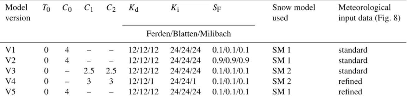
Table 2.Summary of the most important parameters, snowmelt algorithms, and meteorological input data applied in the different model versions.
Model T0 C0 C1 C2 Kd Ki SF Snow model Meteorological
version used input data (Fig. 8)
Ferden/Blatten/Milibach
V1 0 4 – – 12/12/12 24/24/24 0.1/0.1/0.1 SM 1 standard
V2 0 4 – – 12/12/12 24/24/24 0.9/0.9/0.9 SM 1 standard
V3 0 – 2.5 2.5 12/12/12 24/24/24 0.1/0.1/0.1 SM 2 standard
V4 0 – 3 3 12/12/1 24/24/1 0.1/0.1/0.1 SM 2 refined
(b) refined meteorology
cummulated precipitation [mm]
(a) standard meteorology
Figure 8. Accumulated liquid precipitation from 9 October 14:00 UTC to 10 October 20:00 UTC, as regionalized by the hy-drological model using the inverse distant and height regression ap-proaches with the official meteorological stations and the SLF Gan-degg station (cp. Fig. 1), and using(a)the refined meteorology with all available meteorological stations with a correction function and (b)a fixed southwest–northeast interpolation orientation following the topography.
on official meteorological stations and the Gandegg station – had a homogeneous, strongly height-dependent precipitation pattern (Fig. 8a, standard meteorology) with minor internal valley variations. Accordingly, the precipitation sums on the north-facing slope are overestimated (110 mm modeled vs. 42 mm measured at Mannlich, cp. Fig. 4d) and those on the south-facing slope are underestimated. We refined the inter-polation by including all of the meteorological stations avail-able, and we specified a mainly southwest–northeast precip-itation field to correspond with the topography of the valley (Fig. 8b, refined meteorology). The resulting liquid precipi-tation distribution is closer to that described in the local me-teorology section.
The effect of this refined meteorology is analyzed using the model performance in the Milibach tributary catchment. Figure 9 shows the modeled and observed runoff as well as weather and snow depth at the Gandegg meteorological
sta-tion, which is located within the Milibach catchment. The left column summarizes the performance for the standard me-teorology with both snowmelt algorithms (SM1 and SM2) applied, while the right column shows the model output for the SM2 melting using the refined meteorology. For the lat-ter, we also recalibrated the snowmelt parameters to repro-duce the snow cover depletion correctly. As the reference, we used observed snow depth at Gandegg that was converted into SWE by assuming a constant snow density of 0.1 m3s−1
with uncertainty bands of±25 %.
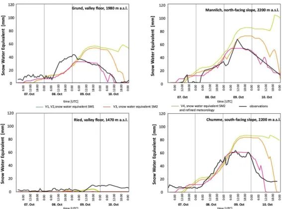
Under standard meteorology and standard parameter set-tings, the SM1 approach is not able to melt the snow cover, because energy input from sensible heat (temperature) was too low at this elevation. Using the SM2 approach snow is melted, but both snow accumulation and snowmelt were overestimated. These limitations were removed in the recal-ibrated model version under refined meteorology. In addi-tion, we increased the water holding capacity from 10 to 20 % of SWE to account for overestimations of discharge at gauges in Blatten and Ferden. Under both SM2 approaches and both water holding capacities, the snow is saturated af-ter the first rainfalls shortly afaf-ter midnight on 10 October. To ensure that the modeled snow dynamic is also correct in the other parts of the valley, we compared the modeled SWE with SWE derived from snow height observations (Fig. 4d). Figure 10 illustrates the snow accumulation and snowmelt for all three model versions at four different stations in the Lötschen Valley. It proves that the recalibrated hydrologi-cal model using SM2 and refined meteorology (magenta line, V4) is able to simulate the snow dynamics, in general, in the entire valley. Smaller differences occur at the south-facing slope (Chumme) with too-intense snowmelt and by underes-timating the small snow cover at Ried. In contrast, SM1 (light green line, V1 and V2) and SM2 (orange line, V3) with stan-dard meteorology cannot reproduce the observed snow dy-namics at any station.
Two conclusions can be drawn from this comparison: (1) the usage of the extended snowmelt module SM2 (V3, orange line, Fig. 9) is necessary to reproduce the snowmelt, and (2) using the refined meteorology and model (V4, right column, Fig. 9) provides a better representation of the snow cover depth and a higher amount of rainfall within the Milibach catchment. However, none of the models are able to reproduce the observed discharge peak (maximum flow is 9.3 m3s−1simulated vs. 32 m3s−1estimated). Only a strong
reduction of the runoff response times for direct-flow and in-terflow from this subcatchment (kdandki, Table 2) leads to a further concentration of discharge and a peak of 24.6 m3s−1
(Fig. 9, dotted orange line). These two parameters are nor-mally calibrated against an observed hydrograph, but as the Milibach catchment is ungauged, the recalibration of the pa-rameters is speculative. A recalibration of the parameterSF
alone as done in V2 was not sufficient to reproduce the dis-charge peak in the Milibach catchment (10.2 m3s−1
Figure 9.Model performances with standard and refined meteorology for precipitation and temperature (top row), snow depth (center row) and runoff (lower row) for the tributary river Milibach using both snow models (SM1 and SM2, model V2 and V3). Shaded grey area indicates the uncertainty origin from unknown snow density (±25 % of 0.1 g cm−3). Dashed violet line depicts the liquid water content in the snow cover. Refined meteorology and snowmelt from latent and sensible heat are able to reproduce both snow cover accumulation and depletion.
Applying this recalibrated model to the entire Lonza catch-ment provides also a good representation of the flood peak at Blatten and Ferden (V4, Fig. 7). However, there are large overestimations in the diurnal melting cycles before the event due to the overestimation of the SM2 melting rates. The re-calibrated model therefore is only valid for the rain-on-snow flood. Still, the reliability of this model version for the time of the flood peak is higher than that of previous versions, as the observed catchment’s internal characteristics, such as precip-itation distribution and snow depletion, are incorporated.
The comparison of the recalibrated model with the stan-dard model revealed that the processes during the flood event were far from standard conditions as model parame-ters, snowmelt algorithms, and input data sets differ between both model versions (Table 2, V1, V4). These differences point to the processes relevant during the flood event: firstly, the recalibration during the flood event demonstrated the
im-portance of both latent and sensible energy in the melting process, as suggested by the analysis of the local meteorol-ogy. Moreover, the refinement of the meteorology was im-portant for representing the strong heterogeneous runoff pat-tern, which proves the strong regional concentration of pre-cipitation during this flood that official meteorological sta-tions alone are unable to capture. Finally, model parameters related to response times and runoff generation (kd andki,
Table 2) have to be set in a way that rainfall and snowmelt directly contribute to the discharge with a higher runoff con-centration than under standard conditions.
Still, some limitations remain in the representation of the flood peak of Milibach (25 m3s−1 simulated vs. 32 m3s−1
Figure 10.Snow model performance of standard (V1 and V2, green lines), and enhanced snow modules (V3, orange lines), as well as recalibrated SM2 under refined meteorology (V4, magenta lines) in terms of SWE at four different meteorological stations (Reid, Grund, Mannlich, Chumme, see Fig. 1) representing different altitudes and expositions. Observations (black line) are derived from snow height measurements assuming a snow density of 0.1 g cm−3.
Milibach catchment led to a flood peak of 31 m3s−1 (not
shown here), but resulted in an overestimation at the gauge Lonza, Ferden, too.
Assuming that this recalibrated model captures the main processes, the water fluxes and the hydrological runoff coef-ficients are calculated for this event using the SM2 model un-der standard meteorology and parameters and unun-der refined meteorology with recalibrated parameters (Table 3). For the two larger catchments differences between the versions are small, with a little less snow and runoff applying the re-fined meteorology. However, for the Milibach catchment, the changes are significant. The refined meteorology shifts the proportions of solid and liquid precipitation, reducing the in-fluence of snowmelt and enhancing direct runoff from rain-fall. As the snow cover was not entirely melted and soils were filled up during the flood event, the models suggest that there was even the potential for an even higher flood. Considering only modeled rainfall and runoff as the input, the runoff co-efficient9 was calculated as9 >1, which emphasized the strong contributing role of snow for this event. Of the flood water, 30 % originated from snow in each of the (sub-) catch-ments using the optimal model configuration. Snowmelt con-tribution under the standard meteorology and SM2 approach is remarkably high (at least 62 %).
To conclude, using standard meteorology, the peak op-timized hydrological model (V2) is able to approximately reproduce the flood peak at the catchment scale. But a de-tailed analysis at the subcatchment scale showed that these reproductions were due to the wrong reasons: using uni-formly distributed precipitation amounts in the catchment and a runoff promoting snow cover (SF=0.9) resulted in a correct representation of the flood peak of the Lonza, but failed to reproduce the uneven distributed flooding in the trib-utary rivers and strongly underestimated the flood peak at the Milibach. The optimal hydrological model (V4) reproduced flood peaks at the catchment and subcatchment scales rea-sonable well, but requires a meteorological refinement and an extensive recalibration of model parameters.
3.4 Predictability of the event
Table 3.Water fluxes, storages and characteristic values during the peak flow from 6 to 10 October 2011 for SM2 melt modules under standard and refined meteorology and parameters.
Ferden (140 km2) Blatten (78 km2) Milibach (3.3 km2)
Meteorology
Standard Refined Standard Refined Standard Refined
Rain [mm] 93.6 94.5 75.5 77.4 92.6 167.9
Snow [mm] 124.2 104.3 122.6 121.8 103.9 84.4
Total runoff [mm] 102.2 95.7 92 80.3 109.3 188.4
Direct flow [mm] 39.7 39.6 36.5 31.2 45.8 99.4
Interflow [mm] 92.5 55.9 55.4 48.9 63.5 88.8
Base flow [mm] 0 0.2 0 0.2 0 0.1
Max. snow cover [mm] 85.3 62.3 102.9 79.6 97.3 72.1
Snow cover after event [mm] 21.8 34.9 43.7 67.8 22.9 12.8
Change in snow cover [mm] −63.5 −27.4 −59.2 −11.8 −74.4 −59.3
Change in soil moisture [mm] 6.7 33.2 6.3 29.4 7.1 46.9
Rainfall–runoff coefficient [1/1] 1.09 1 1.22 1 1.18 1.1
Snowmelt–runoff ratio [1/1], Jasper et al. (2002) 0.62 0.3 0.64 0.1 0.68 0.3
meteorology (rain: blue bars, snow: yellow bars, temperature curve in black). COSMO-2 data (12 h before flood peak) un-derestimate both the temperature increase and the precipi-tation amount in the morning of 10 October, resulting in a strong underestimation of the flood peak (25 m3s−1, 18 h in advance; 24.8 m3s−1, 12 h in advance; and 35 m3s−1, 6 h
in advance at Lonza, Blatten). The forecast 6 h in advance resulted at least in a flood peak at the 2-year-return level (35 m3s−1). This corresponds to a medium hazard level at
Lonza, Blatten. Comparing the total precipitation sums on 10 October of the COSMO-2 forecast data (12 h in advance, Lonza at Ferden catchment: 71.7 mm, Milibach catchment: 72 mm), standard meteorology (Lonza at Ferden catchment: 90.1 mm, Milibach catchment: 87.1 mm), and refined mete-orology (Lonza at Ferden catchment: 112.8 mm, Milibach catchment: 164.7 mm), and regarding that using the standard meteorology a higher flood peak was achieved (Fig. 7, left column), the underestimation of precipitation is not the only crucial deviation. The lower temperatures in the night and morning of 10 October led to a higher proportion of snow-fall instead of rainsnow-fall on 10 October and reduced snowmelt. In addition, it should be noted that using the optimized hy-drological model and the best forecast data available (6 h in advance), the predicted flood peak at Lonza, Ferden, was still underestimated by at least 50 %.
4 Discussion
Extreme flood events typically result from adverse spatial and/or temporal combinations of factors: spatially, when in-tense weather occurs over particularly vulnerable regions (sealed, saturated, steep); temporally, when a particular se-quence of (not necessarily extreme) weather conditions result in an extreme flood. In the present case, a temporally adverse
sequence of weather conditions can be traced back to the suc-cessive interaction of two (a cold and a substantially warmer) air masses with the complex Alpine topography. Compared to a climatology of ERA-Interim reanalysis October temper-atures, the temperatures of the air masses were anomalous but not extreme. The very rapid transition between the two air masses was, however, highly unusual. The amount of mois-ture transported towards the Alps during the rainfall event was exceptional. This moisture was transported over the At-lantic and around the Azores high in a narrow corridor of moist air that fulfills the criteria to be called “atmospheric river” (AR, see e.g., Bao et al., 2006; Ralph and Dettinger, 2011).
While ARs are known to cause river flooding, especially on the west coast of North America (Ralph et al., 2006), little focus has been placed on the effects of ARs in Europe. Knip-pertz and Wernli (2010) and Stohl et al. (2008) showed the presence of ARs in Europe, but linking these wet air masses to floods has seldom been performed for that region. Re-cently, Lavers and colleagues proved that major flood events in Great Britain (Lavers et al., 2011) and annual maxima of precipitation in western Europe (Lavers and Villarini, 2013) are directly linked to AR. Stohl et al. (2008) were able to relate two flood events to ARs that were formed by extrat-ropical transitions of textrat-ropical cyclones.
This flood event is not only a result of the high precipi-tation amounts brought upon the Alps by an AR; it is also a result from the presence of fresh snow and of the intense tem-perature increase that accompanied the moisture. The impor-tant role of the freezing level and snow-covered area during rain-on-snow events was stressed by McCabe et al. (2007). Minimum and maximum temperature levels must suit the el-evation distribution of the affected snow-covered valley to become problematic. Here, the 9 K temperature increase dur-ing the night of 9–10 October activated the meltdur-ing of the snow cover up to an elevation of 3000 m a.s.l., which is 81 % (1400–3000 m a.s.l.) of the valley area. The snow cover in the Lötschen Valley was hence very sensitive to this temper-ature increase and, accordingly, 30 % of the total runoff water originated from snowmelt (Table 3).
In addition to this synoptic-scale meteorological situation, the intensity of the rain-on-snow event was highly variable at the valley scale. Evidence points to the important role of a cavity circulation (upslope winds and formation of a sur-face cloud). This interpretation is consistent with findings of several other studies where seeder–feeder effects are known to cause significant local enhancements of the precipitation amounts (e.g., Roberts et al., 2009; Gray and Seed, 2000). In Pennsylvania, Barros and Kuligowski (1998) found that “leeward-side effects” enhance the local precipitation during rain-on-snow events and that there is a correlation between “leeward-side effects” and significant hydrological flooding. The cavity circulation not only enhanced the rainfall amount but also brought warm and moist air masses in di-rect contact with the snow cover, resulting in intensified
snowmelt through sensible and latent heat transfer. Espe-cially wind speed and humidity are essential for an enhanced snowmelt as indicated by the melting equations: assuming a relatively small degree-day factor of 0.5 for latent heat melt-ing and only 1 m s−1wind speed, 40 mm of rainfall are nec-essary to generate the same amount of snowmelt from rain-fall as from condensation. This relation gets even more un-balanced with higher wind speeds and degree-day factors. Strong surface winds, warm temperatures and high humidity indeed proved to contribute directly to high snowmelt rates recorded in catastrophic rain-on-snow floods like in 1996 in the Pacific northwest (Marks et al., 1998) and in northern Pennsylvania (Leathers et al., 1998). Our findings are con-sistent with these studies.
The application and the recalibration of the hydrological model for this flood reconstruction confirmed the observed rapid response of the catchment to the rainfall and snowmelt. We emphasize the importance of latent energy for the rapid snowmelt process because only the snow module considering sensible-andlatent-heat flow (SM2) was able to reproduce the snow depletion. The importance of latent and sensible heat for snowmelt during rain-on-snow events is consistent with results from other studies, e.g., (Marks et al., 1998), in which an energy-balance model was applied to a rain-on-snow event.
Besides the strong energy input, snow cover structure and lateral flow processes are crucial in explaining the rapid runoff. Kroczynski (2004) compared two similar rain-on-snow events with different consequences, one leading to a major flood and one without any flooding. He argued that the cause for the major flood was the prior condition of the snow cover (a ripened snow cover) that led to a saturated snow cover. Singh et al. (1997) experimentally showed that saturated snow cover produces a very rapid runoff response and maximum melt flow due to the presence of preferential vertical flows.
In the present case, the snow cover was not ripe but rather fresh. As observational data on liquid water content are missing, we refer to the model data to estimate the snow cover saturation: the snow cover up to 2700 m a.s.l. was modeled to be saturated shortly after midnight on 10 Oc-tober by the lighter preceding rainfall, so the subsequent heavy rainfall (on the morning of 10 October) fell on a sat-urated/ripe snow cover. This is although the water holding capacity was increased from 10 to 20 % – according to Jones et al. (1983) a reasonable value during intense snowmelt pe-riods. The WSL/SLF (Institute for Snow and Avalanche Re-search; Jonas et al., 2013) analyzed the role of the snow cover for the flood event in detail using the 1-D SNOWPACK model. Confirming our model results, they concluded that the snow cover up to an elevation of 2000 m a.s.l.in the Lötschen Valley was saturated when rain started to fall.
and just below the snow even under unsaturated snow cover conditions and without percolation to the soil surface. Kattel-mann and Dozier (1999) emphasized the heterogeneity of a snow cover even with only few major stratigraphic layers and report on nonuniformly distributed channels in the snowpack – vividly described as a “swiss cheese”. For the present rain-on-snow event, the importance of these lateral flow paths has to be assumed – giving the intense rainfall, the steep slope of the catchment (32◦ on average) enforcing lateral flows and the rapid and concentrated runoff observed.
These very dynamic and rapid melting and lateral runoff processes are not captured by the rather conceptional, static vertical process description of WaSiM with fixed water hold-ing capacity, infiltration into the soil, and no lateral routhold-ing. The only possibility to regard these processes in WaSiM is the parameter SF to prevent infiltration processes and an ad-justment of the routing parameters in the Milibach subcatch-ment to account for the faster runoff generation and concen-tration. In the present case this adjustment was found essen-tial to reproduce the flood peak, a recalibration of the param-eter SF was not sufficient (not shown here).
However, there are limitations to this recalibration: Rapid snowmelt release from snow cover is not reproduced in a physical manner in the hydrological model WaSiM-ETH, but rather captured by changing these conceptional parameters. The recalibrations of the runoff time in the Milibach catch-ment are especially uncertain as they are not validated with constantly measured discharge and they refer only to the pro-cess during rain-on-snow events.
Furthermore, missing runoff data at the gauge for the Lonza at Ferden (Fig. 7) make the determination of the flood peak uncertain. This is even more important as this gauge covers two-thirds of the Lötschen Valley and hence repre-sents most of the flood causing processes. However, due to the temporal agreement of the flood peak of different model versions and the last data point measured at Ferden, we as-sume that the flood peak was covered.
Finally, we were unable to simulate the estimated runoff-peak of 32 m3s−1in the Milibach catchment. This might be
partly due to an underestimation of the measured rainfall, or it might be due to the model’s limitations to describe the runoff processes from snow cover appropriately. In addition, because the flood peak was estimated by field observations, the estimated value itself is uncertain, even though it was per-formed by an expert (unpublished data, Geoplan Naturge-fahren). Despite the extensive observations available in the Lötschen Valley and even though we were able to reproduce the course of the event with a hydrological model, the exact flood magnitude in the Milibach catchment and the response time of the catchment remains uncertain due to uncertainties of observations and in the hydrological model.
Using the COSMO-2 forecast data as input to drive the optimized hydrological model, we found that the flood peak was substantially underestimated; the forecasted peak flow was a 2-year event (Lonza at Blatten gauge: 35 m3s−1).
Comparing this underestimated flood peak (60 m3s−1,
Fig. 11) from a “perfect” hydrological rain-on-snow model under forecasted meteorology with the flood peak gained from the standard hydrological model under “perfect” me-teorology (75 m3s−1, Fig. 7 right column), it can be con-cluded that the slightly greater error originated from the im-perfect meteorological forecast data. We found a combina-tion of insufficient precipitacombina-tion and a weaker temperature increase than observed (during the night of 9–10 October) that resulted in insufficient runoff. A reason for this un-derestimation might be an unrealistic representation of me-teorological processes by COSMO-2 at a small scale like the Milibach catchment (3.3 km2). The model performance of the COSMO-2 precipitation has been evaluated against coarser resolution models and radar-based observations by Weusthoff et al. (2010). They found COSMO-2 to represent the convective precipitation such as the precipitation in the present study much better than coarser NWPs. Strikingly, the spatial pattern of the COSMO-2 precipitation (not shown here) was in good agreement with our station measurements. However, the temperature increase and precipitation amounts were not well predicted. This underlines findings by Jasper et al. (2002), who emphasized the gross effect of small devia-tions in temperature and precipitation forecast data on hydro-logical projections.
While the results of this case study are primarily limited to the catchment, the special meteorological situation causing the flood and the special model configuration of the hydro-logical model applied, the question of which findings can be transferred to other areas arises. Viviroli et al. (2009) showed that model parameters can be regionalized even for flood cal-ibrations. However, it remains unclear whether this regional-ization procedure holds also true for model settings repsenting this rain-on-snow event. But Hermi et al. (2013) re-analyzed the same flood event in different Swiss catchments with the hydrological model PREVAH (Precipitation Runoff Evapotranspiration HRU) and confirmed our finding that the uncorrected standard model was not able to adequately repro-duce the flood event and that runoff response times as well as snowmelt parameters need to be recalibrated to fit the model against observations. It can be argued that these parame-ters and configurations have to be calibrated in general for the presentation of rain-on-snow events, independent from the catchment, the meteorological conditions, and hydrolog-ical model used. Thus, the direct transfer of model param-eters is precarious; however, the information about parame-ters and model settings that need to be changed to capture the main processes involved in rain-on-snow events might remain valid. Further studies are needed to prove the trans-ferability of this information.