Polynomial Representations for a Wavelet Model of Interest Rates

(1)

Polynomial Representations for a Wavelet

Model of Interest Rates

Dennis G. Llemit

Department of Mathematics, Adamson University 1000 San Marcelino Street, Ermita, Manila, Philippines

[email protected]

Date Received: December 22, 2015; Date Revised: January 15, 2016

Asia Pacific Journal of Multidisciplinary Research

Vol. 3 No.5,62-71 December 2015 Part III P-ISSN 2350-7756 E-ISSN 2350-8442

www.apjmr.com

Abstract - _{In this paper, we approximate a non}–_{polynomial function which promises to be an} essential tool in interest rates forecasting in the Philippines. We provide two numerical schemes in order to generate polynomial functions that approximate a new wavelet which is a modification of Morlet and Mexican Hat wavelets. The first is the Polynomial Least Squares method which approximates the underlying wavelet according to desired numerical errors. The second is the Chebyshev Polynomial approximation which generates the required function through a sequence of recursive and orthogonal polynomial functions. We seek to determine the lowest order polynomial representations of this wavelet corresponding to a set of error thresholds.

Keywords: Chebyshev polynomials, polynomial least squares, Torre – Escaner wavelet

INTRODUCTION

A wavelet is a mathematical function that is used to divide a given function or a continuous- time signal into different scale components. Since wavelet transforms are representation of functions similar to those of Fourier transforms, they are used in data compression and signal processing. Over the years, wavelets have been employed in research undertakings in a broad range of fields from electrical engineering and computer science to economics and finance. The utility of wavelets lie in their capacity to make sense of real world data which are mostly non-stationary, non-periodic, and noisy. The data are transformed such that analyses and inferences on them can be done easily.

Such transformation mechanism is not inherently unique to wavelets. Joseph Fourier conceptualized the Fourier transform in 1807. The method uses orthogonal basis functions to represent continuous and periodic functions. For � ∈ ℝ,

1≤ �< +∞, let

� ∈ �

be the signal function to be analyzed. Then its Fourier transform is defined as

� = � +∞

−∞

−2� � _�

where � is in Hertz.

Fourier transform was a success in function transformation but it has a major shortcoming. It is not compactly supported in time. Thus, it is not a suitable transformation for non-stationary data. The Short Time Fourier Transform (STFT) was conceptualized to correct this drawback. It is given by

�, = � ∗ � − � −2� � �

where (�) is the windowing function, � is the time axis, and � are frequency and translation parameters, respectively, and ∗ is the complex conjugate operator. The STFT is compactly supported in time. However, it uses the same window for the analysis of the entire signal. This brought difficulties in data analyses. If the signal to be analyzed has high frequency components for a short time span, narrow windows are used. But such narrow windows mean wider frequency bands which result to poor frequency resolution. On the other hand, if the signal features low frequency components of longer time span, then a wider window needs to be used to obtain good frequency resolution.

(2)

Llemit, Polynomial Representations for a Wavelet Model of Interest Rates

_______________________________________________________________________________________________________________

63

P-ISSN 2350-7756 | E-ISSN 2350-8442 | www.apjmr.com

Asia Pacific Journal of Multidisciplinary Research, Vol. 3, No. 5, December 2015 have been constructed to suit the needs of a wide

variety of phenomena and applications.

In 2010, Noemi Torre and Jose Maria Escaner, IV, developed a new wavelet which we call the Torre – Escaner Wavelet. This new wavelet fits historical data of Philippine 90 – day T – bill rates from 1987 up to 2008. It was constructed using the Morlet and Mexican Hat wavelets and logically inherits their intrinsic properties. The Morlet wavelet is known to offer improved detection and localization of scale over the Mexican Hat. On the other hand, the Mexican Hat wavelet provides better detection and localization of patch and gap events over the Morlet wavelet.

The Torre – Escaner wavelet is given by

� = 2 3�

−1

4₍₁− _1.1�₎2 − (1.1�)2

2 7.7�₍₁₎

where t stands for time and W(t) for frequency.This new wavelet fits historical data of Philippines 90 – day T – bill rates and can be potentially used to model Philippine interest rates according to Torre and Escaner [1].

In the areas of computing and numerical analysis, polynomial functions receive preferential treatment. This is because their structures, being based on elementary operations of addition and multiplication, are simple to humans and to computers. In the context of computational, time and space complexities, polynomial functions are much efficient compared to their non – polynomial counterparts. That is why, if possible, non-polynomial functions are transformed as polynomials via numerical approximation methods. As is the case with such approximation techniques, there is always the error trade – off. That is, the error varies inversely to the degree of the approximating polynomial.

OBJECTIVES OF THE STUDY

In this paper, we intend to

(a) represent the Torre – Escaner wavelet by a polynomial function �(�) via numerical methods; and

(b) determine the root-mean-squared errors, � = 1 ∥ � − � (�)∥₂, of these polynomial representations.

We are interested in polynomial functions as approximations for the Torre – Escaner wavelet for

three reasons. Firstly, polynomial functions are generally simple and easy to manipulate. Secondly, polynomial functions are algorithmically easy to implement and computationally efficient. Note that these two are the reasons why we only want a polynomial approximation of practical degree. Although a plethora of numerical schemes can easily give an approximation for (1), they are mostly higher ordered that they become impractical for our goal. Thirdly, we want to provide a numerical basis or treatment for the wavelet that can model Philippine T – bill rates.

METHODS

We employ techniques and methods provided in Numerical Analysis such as Polynomial Least Squares (PLS) and Chebyshev Polynomial approximations to construct the approximating or interpolating function � (�).

Polynomial Least Squares Approximation

For the Polynomial Least Squares (PLS) approximation, we seek to construct a degree n polynomial,

� � = ₀+ ₁�+ ₂�2+ + � (2)

from the Torre – Escaner wavelet W(t), such that the root- mean squared error, � is as small as possible,

i.e.,

� = 1 ∥ � − � � ∥₂

< (3)

Let

� 0, 1,…, = � −=1 � � 2

= [ � − ₀− ₁� − ₂�2− − � ]2

=1

� 0

= 0,

�

(3)

To minimize � , we set the following:

� _{= 0,}

and solve the subsequent equations

� 0

=−2 � − ₀− ₁� − ₂�2− − � = 0 =1

,

� 1

=−2 � − ₀− ₁� − ₂�2− − � � = 0 , =1

�

=−2 � − ₀− ₁� − ₂�2− − � � = 0

=1

,

which simplifies to

0 1 +

=1

1 � +

=1

� = (�)

=1 =1

,

0 � +

=1

1 � 2+

=1

� +1₌ ₍_�₎_� =1

,

=1

0 � +

=1

1 � −1+

=1

� 2 ₌ ₍_�₎_� =1

=1

. (4)

According to Atkinson and Han [2], (4) is a system of normal equations which is equivalent to

= (5)

where

=

1 �1 �12 1 �₂ �₂2

1 � �2

… �1 … �2

… �

and

=

(�1) (�₂)

(4)

_______________________________________________________________________________________________________________

65

Asia Pacific Journal of Multidisciplinary Research, Vol. 3, No. 5, December 2015 Expression (5) is also equivalent to

1 =1 � =1 … _� =1 � =1 �2 =1

… � +1

=1

� +1 =1

� +2 =1

… �2 =1 0 1 = (�) =1 (�)� =1

(�)�2 =1

,

which can be expressed as

= (6)

where = 1 =1 � =1 … _� =1 � =1 �2 =1

… � +1

=1

� +1 =1

� +2 =1

… �2 =1 ′ = 0 1 , and = (�) =1 (�)� =1

(�)�2 =1

.

(5)

Chebyshev Polynomial Approximation

Instead of monomial basis, Chebyshev Polynomial approximation uses different bases vectors. Let

� = cos �= cos (arccos(�)) (7)

where −1 ≤ � ≤1. We know that

cos( + 1)�+ cos( −1)�= 2 cos �cos�.

Thus, we have

+1 � = 2� � − −1 � . (8)

Hence, the basis vector is of the form { 0 � , 1 � , 2 � ,… , � } which is also a basis vector of polynomials in terms of t. According to a theorem by Weierstrass [3], if � � interpolates a given function f (t) on the zeros of +1(�), then

∥ � − � � ∥∞≤ 2

−

+ 1 !

max

�0≤ � ≤ �

+1_�₍₉₎

where � ∈ −1,1.

This theorem guarantees that a good fit of f (t) can be found. Hence it is imperative to determine the zeros of +1 � . That can be done by simply setting (7) to zero and solving for the corresponding � values.

cos �= 0

�= 2 + 1 �

2, = 0,1,2,…, −1 ,

� = 2 + 1 �

2 , = 0,1,2,…, −1 .

Let

� = cos�= cos( 2 + 1 �

2 ) ; = 0,1,2,…, −1 (10)

be the kth zero of (7). Then the set generated by (10) is called the set of Chebyshev nodes of (7).

Next, we note that since { ₀ � , ₁ � , ₂ � ,…, � } is a basis for the set of polynomials, then the set is linearly independent and (�) is orthogonal to (�) for ≠ from Kolman and Hill[4]. Hence, we can set

(6)

_______________________________________________________________________________________________________________

67

Asia Pacific Journal of Multidisciplinary Research, Vol. 3, No. 5, December 2015

a linear combination of these basis vectors. Thus, we need to determine each coefficient to come up with the Chebyshev polynomial approximation � (�) for � . � (�) interpolates � at the (n +1) Chebyshev nodes so that at every node � ,

� =� � .

Hence,

� � = (�) (�) =0

=0 =0

= � (orthogoninality of and )

=0

=1 2 + 1

where =1

2 + 1 .

Thus, the coefficients can be obtained by

= 2

+ 1 � � (12) =0

where� = cos + 1 2 �

+1 .

RESULTS AND DISCUSSION

After considering several choices, we come up with the common interval of interest for (1). The interval is [-1,1] because this is the only interval in which our Matlab codes give quality results. For one, the graph outside [-1,1] explodes. For comparison purposes, we set a maximum root- mean square error, � , of 0.10 corresponding to 10 percent. This threshold might be considered large but setting a very small value might result in very high polynomial degrees.

Least Square Approximation Results

Using Matlab, the minimum degree of the approximating polynomial is = = 20. For values larger than 20, the Matlab program returns a warning note that the solution to the matrix system (6) may be inaccurate. This is because L is a Hilbert matrix [5]. As the matrix becomes large, its determinant tends to zero. Thus L becomes non- invertible.

For this particular degree, the Matlab program returns the polynomial representation for (1): �20 � = 4.2−0.01 �20+ 9.32 �19+ −35.47 + 0.03 �18

+ 0.01−67.28 �17+ 144.3 + 0.06 �16 + −0.02 + 234.72 �15 + −376.03 + 0.07 �14+ 0.03−526.04 �13+ 691.51−0.05 �12 + 0.02 + 827.98 �11+ −914.14 + 0.02 �10+ 0.01−921.35 �9 + 842.72−0.01 �8+ 692.78 �7−505.15�6−321.48 �5

(7)

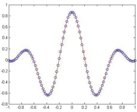
Its graph is

Figure 1: Graph of �20(�) with W(t) in circles

However, its root- mean- squared error is

� = 1 ∥ � − �₂₀ � ∥₂= 0.8014,

much bigger than the threshold root- mean squared error.

Chebyshev Polynomial Approximation Results

For the Chebyshev Polynomial approximation, Matlab was able to find a polynomial approximation that satisfies the threshold error. In fact, it was able to find more than one polynomial in the interval [-1,1]. Since we want a polynomial of minimum degree, we only get the three lowest, in terms of degree, polynomial representation.

The lowest degree polynomial representation is

�10 � = −97.36�10+ 54.93 �9+ 284.32�8 −145.35�7−304.26�6+ 133.73 �5

142.08�4−48.64 �3−25.73�2

(8)

_______________________________________________________________________________________________________________

69

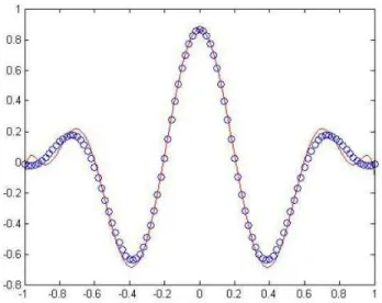
Asia Pacific Journal of Multidisciplinary Research, Vol. 3, No. 5, December 2015 Its graph is

and the corresponding root- mean- square error is

� = 1 ∥ � − �₁₀ � ∥₂= 0.0792,

which is less than the threshold error 0.10.

The next lowest degree polynomial representation is

�11 � =−104.19 �11−72.21�10 + 346.99�9 +220.32�8−444.54 �7−246.96�6

+268.81�5+ 120.97�4−73.82�3

−22.97�2+ 6.62�+ 0.81 . (15)

Its graph is

(9)

while its root- mean- squared error is

� = 1 ∥ � − �11 � ∥2= 0.0376,

expectedly lower than �₁₀ � .+

Lastly, the third lowest degree polynomial representation is

�12 � = 100.6�12−82.03�11 −378.5�10 +285.21�9_{+ 571.23}_�8₋_381.68 _�7 −433.14�6_{+ 240.67} _�5_{+ 165.93}_�4

−68.64 �3−26.99�2+ 6.35�+ 0.87. (16)

Its graph is

Its root- mean- squared error is

� = 1 ∥ � − �12 � ∥2= 0.0163,

(10)

Asia Pacific Journal of Multidisciplinary Research, Vol. 3, No.5, December 2015

_______________________________________________________________________________________________________________

71

P-ISSN 2350-7756 | E-ISSN 2350-8442 | www.apjmr.com CONCLUSION

The purpose of this paper was to find polynomial approximations to the Torre- Escaner wavelet with ideal root- mean- squared errors. We first used the Polynomial Least Squares (PLS) approximation scheme and the results showed that the only resulting representation (13) did not satisfy our threshold � .

This meant that PLS failed to provide a good polynomial approximation for (1).

On the other hand, the Chebyshev Polynomial approximation scheme was able to provide good polynomial approximations for (1) at lower polynomial degrees. This is a validation of the “near -minimax” nature of the Chebyshev Polynomial approximation. Under this scheme, the lowest degree polynomial representation for the Torre – Escaner wavelet that satisfied the threshold � was

�10 � = −97.36�10+ 54.93 �9+ 284.32�8 −145.35�7−304.26�6+ 133.73 �5

142.08�4−48.64 �3−25.73�2

5.28 �+ 0.87.

For future works, we would like to examine other polynomial approximation schemes such as the Legendre, Gegenbauer, Jacobi and other orthogonal

polynomials whether they can provide better approximations than the Chebyshev scheme.

REFERENCES

[1] N. Torre and J.M.L. Escaner IV. A New

Wavelet based on Morlet and Mexican Hat Wavelets. Matimyas Matematika, 2010

[2] K. Atkinson and W. Han. Elementary

Numerical Analysis, Third Edition. John Wiley and Sons, New York, 2004.

[3] E. W. Cheney. Introduction to Approximation

Theory. AMS Chelsea Publishing, Rhode Island, 1966.

[4] B. Kolman and D. Hill.Elementary Linear

Algebra. Pearson Education, New Jersey, 2008.

[5] W. Yang, W. Cao, T. Chung, and J. Morris.

Applied Numerical Methods Using MATLAB. John Wiley and Sons, New Jersey, 2005.

Copyrights