UNIVERSIDADE TÉCNICA DE LISBOAI NSTITUTO SUPERIOR DE ECONOMIA E GESTÃO Essays on Wavelets in Economics

(1)

UNIVERSIDADE TÉCNICA DE LISBOA

I

NSTITUTO SUPERIOR DE ECONOMIA E GESTÃO

Essays on Wavelets in Economics

por

António Miguel Pinto de Oliveira Gomes Rua

Júri

Presidente: Reitor da Universidade Técnica de Lisboa Vogais:

- Doutor Luís Catela Nunes, professor associado da Faculdade de Economia da Universidade Nova de Lisboa

- Doutor Paulo Meneses Brasil de Brito, professor associado do Instituto Superior de Economia e Gestão da Universidade Técnica de Lisboa

- Doutor Artur Carlos Barros da Silva Lopes, professor associado do Instituto Superior de Economia e Gestão da Universidade Técnica de Lisboa - Doutor Manuel António da Mota Freitas Martins, professor auxiliar da Faculdade de Economia da Universidade do Porto

- Doutor Luís Francisco Gomes Dias Aguiar-Conraria, professor auxiliar da Escola de Economia da Universidade do Minho

Doutoramento em Economia orientado por:

Doutor Artur Silva Lopes Doutor Luís Catela Nunes

Versãoﬁnal

(2)

Resumo

O objectivo deste trabalho é realçar a utilidade da análise de onduletas em Economia. A análise de onduletas é uma ferramenta muito promissora, pois representa um reﬁnamento da análise de Fourier. Em particular, permite

ter em consideração quer o domínio do tempo quer o domínio da frequência de forma uniﬁcada, ou seja, é possível avaliar simultaneamente como é que

as variáveis estão relacionadas em diferentes frequências e como é que essa relação tem evoluído ao longo do tempo. Apesar do potencial interesse, a análise de onduletas constitui ainda uma ferramenta relativamente pouco utilizada no estudo de fenómenos económicos. O trabalho aqui apresentado pretende contribuir para essa vertente da literatura.

Em particular, a análise de onduletas é usada para avaliar a relação entre o crescimento monetário e a inﬂação na área do euro, dado que o Banco

Central Europeu atribui um papel fundamental para a moeda no contexto da sua estratégia de política monetária. Adicionalmente, é proposta uma medida de co-movimento baseada em onduletas sendo utilizada para estudar o co-movimento, em termos de crescimento, entre as maiores economias da área do euro. Com base nesta medida, também é proposta uma medida de coesão que é usada por sua vez para aferir a coesão entre os países da área do euro e nos Estados Unidos, quer a nível regional quer estadual. No contexto da literatura de economia ﬁnanceira, a relação entre retornos de acções no

mercado internacional é avaliada e é proposta uma abordagem baseada em onduletas para a medição de risco de mercado. Finalmente, a utilidade das onduletas para efeitos de previsão é investigada e a sua interacção com os modelos de factores é explorada.

Palavras-Chave: Onduletas; Tempo-frequência; movimento;

(3)

Abstract

The aim of this work is to highlight the usefulness of wavelet analysis in Economics. Wavelet analysis is a very promising tool as it represents a reﬁnement of Fourier analysis. In particular, it allows one to take into

account both the time and frequency domains within a uniﬁed framework,

that is, one can assess simultaneously how variables are related at diﬀerent frequencies and how such relationship has evolved over time. Despite the potential value of wavelet analysis, it is still a relatively unexplored tool in the study of economic phenomena. The work herein presented intends to contribute to such strand of literature.

In particular, wavelet analysis is used to assess the link between money growth and inﬂation in the euro area, as the European Central Bank

at-tributes a key role to money within the monetary policy strategy. Addi-tionally, a wavelet-based measure of comovement is proposed and used to study the growth comovement among the major euro area countries. Based on this measure, a measure of cohesion is developed and used to investi-gate the cohesion among euro area countries and the cohesion within US at both the regional and state levels. Within theﬁnancial economics literature,

the relationship among international stock market returns is assessed and a wavelet-based approach for measuring market risk is proposed. Finally, one also investigates the usefulness of wavelets for forecasting purposes while bridging such approach with factor-augmented models.

Keywords: Wavelets; Time-frequency; Comovement; Cohesion; Factor

(4)

Acknowledgments

(5)

1 Introduction

Time domain analysis is, far from doubt, the most widespread approach in the literature to study time series. Through such approach, the evolution of individual variables is modelled and multivariate relationships are assessed over time. Another strand of literature, focus on the frequency domain. Fre-quency domain analysis is a complementary tool to time domain analysis. In particular, with spectral analysis, one can investigate the importance of diﬀerent frequency components for the behaviour of a variable and the rela-tionship between variables at the frequency level. Recent work resorting to Fourier analysis includes, for example, A’Hearn and Woitek (2001), Pakko (2004), Rua and Nunes (2005) and Breitung and Candelon (2006).

Wavelets analysis reconciles both approaches, in the sense that both time and frequency domains are taken into account. Hence, wavelets are a very promising tool as they represent a reﬁnement in terms of analysis. As

men-tioned by Ramsey (2002), "Wavelets are treated as a ’lens’ that enables the researcher to explore relationships that previously were unobservable" while "... the ability to apply a new ’lens’ to inspect the relationships in economics and ﬁnance provides great promise for the development of the discipline".

As Lau and Weng (1995) put it, the wavelet transform has the ability to make a time series sing as it decomposes a signal into localized frequencies with the corresponding measure of intensity and duration, analogous to the bass/treble clef, the crescendo/decrescendo and the tempo in a piece of mu-sic.

Despite its potential usefulness, wavelets have been more popular inﬁelds

other than economics. For example, in geophysics, for the analysis of oceanic and atmosphericﬂow phenomena, seismic signals and climatic data; in

medi-cine, for heart rate monitoring, breathing rate variability and bloodﬂow and

(8)

just to name a few (see, for example, Adisson (2002) for a comprehensive overview).

Although there are still relatively few papers in economics resorting to wavelet analysis, such analysis has already shown to provide fruitful insights about several economic phenomena. For instance, the pioneer work of Ram-sey and Lampart (1998a,b) draws on wavelets to study the relationship be-tween several macroeconomic variables, namely money supply and output in the ﬁrst case and consumption and income in the second. Recent work

using wavelets includes, Kim and In (2003, 2005) who investigate the rela-tionship between ﬁnancial variables and industrial production and between

stock returns and inﬂation, respectively, Gençay et al. (2003, 2005) and

Fernandez (2005, 2006) study the Capital Asset Pricing Model at diﬀerent scales, Connor and Rossiter (2005) focus on commodity prices, Wong et al.

(2003), Conejo et al. (2005) and Fernandez (2007) use wavelets for

fore-casting purposes, In and Kim (2006) examine the relationship between the stock and futures markets, Gallegati and Gallegati (2007) provide a wavelet variance analysis of output in G-7 countries, Crivellini et al. (2004),

Crow-ley and Mayes (2008), Gallegati et al. (2008) and Yogo (2008) resort to

wavelets for business cycle analysis, Aguiar-Conrariaet al. (2008) assess the

time-frequency eﬀects of monetary policy in the US and Aguiar-Conraria and Soares (2010) study the relationship between oil prices and industrial production, among others (see also, for example, Crowley (2007) for a recent survey).

(9)

allows one to assess simultaneously how variables are related at diﬀerent fre-quencies and how such relationship has evolved over time. Hence, one is enabled to capture both time and frequency varying features within an

uni-ﬁed framework. Following this line of research, several essays have been done

within this dissertation.

Anotherﬁeld of research where wavelets can also be particularly useful is

for forecasting purposes. In particular, the wavelet multiresolution approach for forecasting purposes consists in several steps. First, the series to be fore-cast is decomposed into its constituent time-scale components. Then, for each time-scale a model isﬁtted and used for forecasting. Finally, an overall

forecast is obtained after recombining the components. This multiresolution approach can outperform the traditional single resolution approach for fore-casting as it is possible to tailor speciﬁc forecasting models to each time-scale

component and thereby enhance the forecasting performance of the series as a whole. Although the potential usefulness of wavelets in forecasting has been recognized, there are very few applications of wavelets for forecasting in economics. This dissertation also intends to contribute in that respect.

The remainder of the text is organised as follows. Firstly, an overview of the main building blocks of wavelet analysis is provided. In particular, in section 1.1, wavelet analysis is motivated by comparing it with the well-known Fourier analysis. Afterwards, in section 1.2, the continuous wavelet transform is discussed as it constitutes the basis for most of the work done while a short presentation of the discrete wavelet transform and multiresolution analysis is done in section 1.3. Note that the following discussion does not intend to be an exhaustive description of wavelet analysis. Instead, the aim is to provide an intuitive and brief overview of the main tools used in this dissertation. The interested reader canﬁnd, for example, in Percival and Walden (2000) an

extensive introduction to wavelets whereas Gençay et al. (2002) discuss the

(10)

(2007) provide a guide for economists with several illustrations and examples (see also Schleicher (2002)). In section 1.4, the dissertation plan is sketched whereas the corresponding essays are presented in chapters 2 up to 7.

1.1 From Fourier to wavelet analysis

The well-known Fourier transform is the conventional method for studying the frequency content of a signal. It involves the projection of a series onto an orthonormal set of trigonometric components (see, for example, Priestley (1981)). In particular, the Fourier transform uses a basis of sines and cosines of diﬀerent frequencies to determine how much of each frequency the signal contains. The Fourier transform of the time series ()is given by

() =

Z +∞

−∞

()− (1)

where  is the angular frequency and − _{= cos(}_₎₋__sin(_₎ _according

to Euler’s formula. In addition, one can write () as

() =

Z +∞

−∞

() (2)

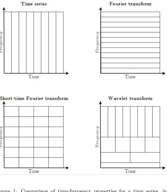
Despite its usefulness, the Fourier transform provides no information about how the frequency content of the signal changes with time, that is, it tells us how much of each frequency exists in the signal but it does not tell us when in time these frequency components exist. To overcome such limitation it has been suggested the so-called short-time Fourier transform (also known as Gabor or windowed Fourier transform). As the name suggests, the basic idea is to use the Fourier transform for short periods of time. It consists in applying a short-time window to the signal and performing the Fourier transform within this window as it slides across all the data.

(11)

by Heisenberg, states that the velocity and the position of a moving particle cannot be simultaneously known to arbitrary precision. In the current con-text, it implies that one cannot exactly know what frequency exists at what time instance. The best one can do is to investigate what spectral compo-nents exist at any given interval of time. Since the resolution in time and fre-quency can not be arbitrarily small, because their product is lower bounded, it results in a trade-oﬀ between time and frequency resolution. This means that for narrow windows one gets good time-resolution but poor frequency resolution whereas for wide windows one gets good frequency resolution and poor time-resolution.

The problem with the windowed Fourier transform is that it uses constant length windows. These ﬁxed length windows give the uniform partition of

the time-frequency plane. When a wide range of frequencies is involved, the ﬁxed time window tends to contain a large number of high frequency

cycles and a few low frequency cycles which results in an overrepresenta-tion of high frequency components and an underrepresentaoverrepresenta-tion of the low frequency components. Hence, as the signal is examined under a ﬁxed

time-frequency window with constant intervals in the time and time-frequency domains, the windowed Fourier transform does not allow an adequate resolution for all frequencies.

In contrast, the wavelet transform uses local base functions that can be stretched and translated with a ﬂexible resolution in both frequency and

(12)

component can be located better in time than a low frequency component. On the contrary, a low frequency component can be located better in fre-quency compared to a high frefre-quency component. However, one should bear in mind that the Heisenberg uncertainty principle is also valid here. So, one cannot expect an improvement of both time and frequency resolution for a given point in the time-frequency plane but one can vary the ratio between the time and frequency uncertainty. As it enables a more ﬂexible approach

in time series analysis, wavelet analysis is seen as a reﬁnement of Fourier

analysis.

(13)

Figure 1: Comparison of time-frequency properties for a time series, its Fourier transform, short-time Fourier transform and wavelet transform.

1.2 The continuous wavelet transform

(14)

(  ) =

Z +∞

−∞

()∗_{ }() (3)

where∗ _{denotes the complex conjugate. Hence, the wavelet transform} decom-poses a time series () in terms of some basis functions (wavelets), _{ }(), analogous to the use of sines and cosines in Fourier analysis. The term wavelet means a small wave. The smallness refers to the condition that this (window) function is ofﬁnite length (compactly supported). The wave refers

to the condition that this function is oscillatory. These basis functions are obtained by translation and dilation of the so-called mother wavelet()and are deﬁned as

 () =

1 √



µ

− 

¶

(4)

where  determines the time position (translation parameter),  is the scale (dilation parameter) and _√1

 is for energy normalization across the diﬀerent

scales1_{. The term translation is related to the location of the window, as}

the window is shifted through the signal (see Figure (2)). The scale refers to the width of the wavelet. By changing the scale parameter, one gets compressed and stretched versions of the mother wavelet. If  1 then the wavelet one will get is compressed; the wavelet corresponding to  = 1 is the mother wavelet; if  1 then one gets a stretched version of the mother

wavelet (see Figure (3)). In terms of frequency, low scales by a compressed wavelet function capture rapidly changing details, that is high frequencies, whereas higher scales by a stretched wavelet function capture slowly changing features, that is, low frequencies.

1_{In particular, the term} 1

√

 makes the variance of the scaled mother wavelet equal to

(15)

Figure 2: Wavelet translation:  = 0 (black solid line),   0 (gray solid

line),  0 (black dashed line).

Figure 3: Wavelet dilation:  = 1 (black solid line),   1 (gray solid line),

 1 (black dashed line).

To be a mother wavelet, (), must fulﬁl certain criteria:

(16)

Z +∞

−∞

()= 0 (5)

that is, the average value of the wavelet in the time domain must be zero;

)its square integrates to unity, Z +∞

−∞

2() = 1 (6)

which means that () is limited to an interval of time;

)and it should also satisfy the so-called admissibility condition,

0  =

Z +∞

0

¯ ¯ ¯b()¯¯_¯2

  +∞ (7)

whereb()is the Fourier transform of(), that is,b() =R_−∞+∞()−__,

so as to allow for the reconstruction of the signal without loss of information. As with its Fourier counterpart, there is an inverse wavelet transform, deﬁned as

() = 1



Z +∞

−∞

Z +∞

−∞

 ()(  )

 

2 (8)

which allows to recover the original series, (), from its continuous wavelet

transform.

Likewise in Fourier analysis, several interesting quantities can be deﬁned

in the wavelet domain. For instance, one can deﬁne the wavelet power

spec-trum as|(  )|2. It measures the relative contribution at each time and at

each scale to the time series’ variance. In fact, the wavelet power spectrum can be integrated across  and to recover the total variance of the series as

follows

2_ = 1



Z +∞

−∞

Z +∞

−∞

|(  )|2

 

(17)

Another quantity of interest is the cross-wavelet spectrum which captures the covariance between two series in the time-frequency space. Given two time series ()and (), with wavelet transforms (  )and (  ) one

can deﬁne the cross-wavelet spectrum as (  ) = (  )∗(  ). As

the mother wavelet is in general complex, the cross-wavelet spectrum is also complex valued and it can be decomposed into real and imaginary parts.

In a similar fashion as in Fourier analysis, one can deﬁne the wavelet

squared coherency as the absolute value squared of the smoothed cross-wavelet spectrum, normalized by the smoothed cross-wavelet power spectra

2₍_{  }_{) =} |(−1(  ))| 2

¡−1_|_

(  )|2

¢

¡−1_|_

(  )|2

¢ (10)

where ()denotes smoothing in both time and scale (see, for example,

Tor-rence and Webster (1999)) and the factor−1 _{is used to convert to an energy}

density. As well as in Fourier analysis, smoothing is also required, otherwise squared coherency would be always equal to one (see, for example, Priestley (1981, p. 708)). The reason for this smoothing is that coherency should be calculated on expected values but in most cases this is impossible, as there is only one realisation of the time series and not a sample from the population. The idea behind the wavelet squared coherency is similar to the one of squared coherency in Fourier analysis. The wavelet squared coherency mea-sures the strength of the relationship between the two series over time and across frequencies (while the squared coherency in Fourier analysis only al-lows one to assess the latter). The 2₍_{  }₎ _{is between} ₀ _and ₁ _{with a high}

(low) value indicating a strong (weak) relationship. Hence, through the plot of the wavelet squared coherency one can distinguish the regions in the time-frequency space where the link is stronger and identify both time and fre-quency varying features.

(18)

lead-lag relationship between the variables in the time-frequency space. The wavelet phase is given by

(  ) = tan−1

µ

=((−1_

(  ))) <((−1_

(  )))

¶

(11)

where < and = are the real and imaginary parts, respectively. The re-semblance with the analogue measure in Fourier analysis is clear. Likewise in Fourier analysis, the phase provides information about the lead-lag re-lationship between the two series. However, besides providing information about the lead-lag across frequencies as standard Fourier analysis, the wavelet phase also allows one to assess how such lead-lag relationship has changed over time.

As the wavelet transform at a given point in time uses information of neighbouring data points, the values of the wavelet transform are generally less accurate as the wavelet approaches the edges of the time-series (this region is known as the cone of inﬂuence (see Torrence and Compo (1998)).

The region affected increases with the temporal support (or width) of the wavelet and to minimize such effects several methods have been developed (zero padding, value padding, decay padding, periodization, polynomial fi

(19)

Mexican hat wavelet

Figure 4: Mexican hat wavelet.

Paul wavelet (real part) Paul wavelet (imaginary part)

(20)

Morlet wavelet (real part) Morlet wavelet (imaginary part)

Figure 6: Morlet wavelet.

As mentioned earlier, all wavelets used in wavelet analysis are obtained by translation and dilation of the mother wavelet. There are a number of func-tions that can be used for this purpose. The most commonly used mother wavelet for the continuous wavelet transform is the Morlet wavelet (other mother wavelets include, for example, Paul and Mexican hat wavelets) (see Figures 4 to 6). One of the advantages of the Morlet wavelet is its com-plex nature which allows for both time-dependent amplitude and phase for diﬀerent frequencies. The Morlet wavelet is deﬁned as

() =−14 µ

0

−−

2 0 2

¶

−

2

2 (12)

Since the term − 2 0

2 (known as the correction term, as it corrects for the

non-zero mean of the complex sine of the ﬁrst term) becomes negligible for

(21)

() =−140−

2

2 (13)

Morlet wavelet (real part) Morlet wavelet (imaginary part)

Gaussian envelope Complex sine (real part)

Complex sine (imaginary part)

Figure 7: Real and imaginary parts of the Morlet wavelet for 0 = 6.

One can see that the Morlet wavelet consists of a complex sine wave within a Gaussian (bell-shaped) envelope (see Figure (7)). The normalization fac-tor, −14, ensures that the wavelet function has unit energy. The parameter

0 is the wavenumber and controls the number of oscillations within the

Gaussian envelope. By increasing (decreasing) the wavenumber one achieves better (poorer) frequency localization but poorer (better) time localization. In practice, setting 0 to 6 provides a good balance between time and

fre-quency localization. Since the wavelength for the Morlet wavelet is given by

4

(22)

scale  is almost equal to the Fourier period which eases the interpretation

of wavelet analysis.

1.3 The discrete wavelet transform and

multiresolu-tion analysis

Up to now the discussion has been focused on the continuous wavelet trans-form. In the continuous wavelet transform, the wavelets used are not orthog-onal and the data obtained by this transform are highly correlated. In fact, in a non-orthogonal wavelet analysis an arbitrary number of scales can be used to provide a complete picture. In contrast, the discrete wavelet transform de-composes the signal into a mutually orthogonal set of wavelets.2 _{Hence, the}

discrete wavelet transform uses a limited number of translated and dilated wavelets. The idea is to choose  and so that the information contained in the signal can be summarized in a minimum of wavelet coeﬃcients. Although the discrete wavelet transform can be derived without explicitly relating it to the continuous wavelet transform, one can think of the former as a "dis-cretization" of the latter. The "dis"dis-cretization" of the wavelet representation in (4) can be written as

_() = _q1

₀ 

Ã

₋00

0

!

(14)

where  and are integers that control the wavelet dilation and translation,

respectively. The scale discretization is given by  =₀ and the translation

discretization corresponds to =00 where0 1 and0 0. Note that

the size of the translation step, ∆ = 00, is proportional to the wavelet

2_{There are other variants of the wavelet transform such as, for example, the maximal}

(23)

scale ₀. Typically, one sets 0 = 2 and 0 = 1 which renders a dyadic

grid, that is, the sampling of both the frequency and time axis is dyadic. This implies that the discrete wavelet transform is calculated only at dyadic scales, that is, at scales 2_{, and within a given dyadic scale one picks times} _

that are separated by multiples of 2_ _{In this case the maximum number of}

scales that can be considered is limited by the total number of observations

 (that is,  is the maximum integer such that  _≤ log(_log(2))). Naturally, the

number of translations within a given dyadic scale is also upper bounded by the duration of the signal.

Substituting0 = 2and 0 = 1into equation (14) one gets the following

discrete wavelet

_() = √1 2

µ

₋2_

2

¶

(15)

Discrete wavelets are usually chosen to be orthonormal through an appropri-ate choice of the mother wavelet, that is,

Z +∞

−∞

_()∗_() =

½

1 if  = and =

0 otherwise (16)

This means that the discrete wavelets are orthogonal to their own dilations and translations and normalized to have unit energy.

Drawing on its spectral properties, the wavelet function can be seen as a band-pass ﬁlter. Since for every stretch of the wavelet in the time domain

with a factor of 2 the corresponding spectrum bandwidth is halved, one

would need an inﬁnite number of wavelets to cover the entire spectrum. To

overcome such problem, one has to resort to the so-called scaling function (or father wavelet). The scaling function acts like a low-passﬁlter and, therefore,

it is associated with the smoothing of the signal. In this way, the smooth and low-frequency part of the series is captured by the father wavelet (),

(24)

wavelet ().

Hence, the discrete wavelet transform makes it possible to decompose a time series into its constituent multiresolution components. The orthogonal wavelet series approximation to a time series () is deﬁned by

() =X



()+

X



()+

X



−1−1()+· · ·+

X



11()

(17) where  is the number of multiresolution levels (or scales) and  ranges

from one to the number of coefficients in the corresponding component. The coefficients , , −1, , 1 are the wavelet transform coefficients,

which are given by

 =

Z

()_() (18)

 =

Z

()_(),  = 12  . (19)

These coeﬃcients give a measure of the contribution of the corresponding wavelet function to the signal.

The functions () and () are generated from  and  through

scaling and translation as follows

_() = 2−2

µ

−2_

2

¶

(20)

and

_() = 2−2

µ

₋2_

2

¶

,  = 12  . (21)

In a more synthetic way, equation (17) can be rewritten as

(25)

where () = P_() and () = P_() for  = 12  

are the smooth and detail components, respectively. The expression (22) represents the decomposition of () into orthogonal components, (),

(),−1(),...,1(), at diﬀerent resolutions and constitutes the so-called

wavelet multiresolution decomposition. For a level  multiresolution

analy-sis, the wavelet decomposition of the variable  consists of  wavelet details

((), −1(),...,1()) and a single wavelet smooth (()). The wavelet

smooth captures the low-frequency dynamics while the wavelet details rep-resent the higher-frequency characteristics of .

Concerning the wavelet families used in the discrete wavelet transform, there are several alternatives in the literature, namely, Haar, Daubechies, Symmlets, Coiﬂets, among others (see Figure (8)). As stressed by Crowley

(26)

Haar

Daubechies

Symmlet

Coiflet

Mother wavelet Father wavelet

(27)

1.4 Dissertation overview

As mentioned earlier, this dissertation intends to contribute to the literature by providing several essays where wavelet anaysis is used to address impor-tant economics problems. In the ﬁrst essay, "Money growth and inﬂation in

the euro area: a time-frequency view" (see chapter 2), a new look into the relationship between money growth and inﬂation is provided. In the euro

area, there is a particular focus on the link between money growth and inﬂ

a-tion, as the European Central Bank gives a prominent role to the monetary aggregate M3 within the monetary policy strategy. The assessment of such link over the last forty years is done resorting to wavelet analysis. Both fre-quency and time-varying interesting features are found concerning the link between money growth and inﬂation in the euro area. On one hand, the

relationship between inﬂation and money growth is stronger at low

frequen-cies than at the typical business cycle frequency range. On the other hand, such link is more robust at low frequencies over the whole sample period whereas there is only supporting evidence at the business cycle frequencies up to the beginning of the 80’s. Concerning the leading properties of money growth, there seems to be a recent deterioration of money growth as leading indicator of inﬂation in the euro area. All in all, these results highlight the

importance of a regular assessment of the privileged role attributed to the monetary aggregate M3 by the ECB within the two-pillar monetary policy framework for tracking medium to long-term developments in inﬂation.

Another topic of noteworthy interest is the measurement of comovement among economic variables. In the essay "Measuring comovement in the time-frequency space" (published in the Journal of Macroeconomics, 32 (2010)

(28)

the comovement of growth cycles among the major euro area countries over the last three decades is assessed. It is found that the strength of comove-ment of growth cycles among the major euro area countries depends on the frequency and has changed over time.

In order to take on board more than two series when assessing comove-ment, in the essay "Cohesion within the euro area and United States: a wavelet-based view" (with Artur Silva Lopes) (see chapter 4), the measure proposed in the previous essay is extended to the more general case in order to obtain a measure of cohesion in the wavelet domain. Focusing on output growth, the cohesion among euro area countries and the cohesion within US at both the regional and state levels over the last decades is investigated. It is found that cohesion within euro area has been higher at the long-term and business cycle frequencies and it has increased since the mid-90s across all frequencies. On the other hand, cohesion within the US is higher at the typical business cycle frequency range but seems to have decreased since the beginning of the 90’s. Note that this ﬁnding holds at both the regional and

state levels. Moreover, it is found that US cohesion is higher at the regional level than at the state level across frequencies and over time. In addition, besides taking into account the spatial perspective when assessing cohesion, an analysis at the sectoral level is also conducted. Resorting to disaggregated data by eleven sectors for the euro area countries and US regions and states, a noteworthy heterogeneity in the results at the sectoral level is found.

It has already been acknowledged that wavelet analysis can contribute in a non-negligible way to the ﬁnancial economics literature. In this respect,

several work has been carried out. In the essay "International comovement of stock market returns: a wavelet analysis" (with Luis Catela Nunes, pub-lished in theJournal of Empirical Finance, 16 (2009) 632—639) the

(29)

impli-cations in asset allocation and risk management. In particular, the focus is on the major developed economies, namely Germany, Japan, United King-dom and United States over the last four decades. Moreover, by considering the decomposition of the aggregate index in ten sectors, several insights at the sectoral level are also provided. Another contribution to ﬁnancial

eco-nomics is the essay "A wavelet-based assessment of market risk" (with Luis Catela Nunes) where a wavelet-based approach is proposed for measuring market risk (see chapter 6). In this way, market risk is allowed to vary both through time and at the frequency level within a uniﬁed framework. The

wavelet counterparts of well-known measures of risk are obtained and to il-lustrate such analysis the emerging markets case over the last twenty years is considered.

Finally, the essay "A wavelet approach for factor-augmented forecasting" (forthcoming in Journal of Forecasting) intends to contribute to the use of

wavelets in forecasting (see chapter 7). In particular, the aim of this essay is to bridge the wavelet approach and factor-augmented models. Factor-augmented models have become quite popular in the recent literature as they allow to handle large data sets in a straightforward and parsimonious way for forecasting purposes. The illustrate such approach, one focus on the short-term forecasting of GDP growth for the major euro area countries, namely Germany, France, Italy and Spain. Among the several alternatives considered, it is found that the best performing procedure is to combine the wavelet approach and factor-augmented models. In particular, for the one-quarter ahead horizon, the forecasting gains are quite noteworthy and the

(30)

2 Money growth and in

_ﬂ

ation in the euro

area: a time-frequency view

2.1 Introduction

As it is well known, the role of money for central banks has changed over the last decades. After the breakdown of the Bretton-Woods system of ﬁxed

exchange rates which provided a nominal anchor for monetary policy, several industrialized countries, including the United States, Canada, the United Kingdom, Germany and Switzerland, adopted the monetary targeting in the 1970s (see, for example, Bernanke and Mishkin (1992) and Mishkin and Posen (1997)). However, the monetary targeting pursued by most central banks was not successful in controlling inﬂation which led them to abandon such

strat-egy starting in the early 1980s. Germany and Switzerland are noteworthy exceptions, with the Bundesbank and the Swiss National bank engaging in monetary targeting for over twenty years (see, for example, Bernanke and Mihov (1997) and Issing (1997) for the former and Rich (1997, 2003) for the latter). The abandon of explicit monetary targeting and the growing in-stability of the relationship between monetary aggregates and goal variables such as inﬂation (see, for example, Estrella and Mishkin (1997)) led to a less

inﬂuential role of money in the policy process. In the early 1990s, inﬂation

targeting wasﬁrst adopted by industrialized countries such as New Zealand,

Canada and the United Kingdom (see, for example, Leiderman and Svens-son (1995) and Bernanke et al. (1999)) and since the late 1990s, it has been

adopted in a number of emerging market and developing countries (see, for example, Batini et al. (2006)).

In contrast with the US Federal Reserve and many inﬂation targeting

(31)

policy strategy. As it is well known, the primary objective of the European Central Bank is to maintain price stability which is deﬁned as a year-on-year

increase in the Harmonised Index of Consumer Prices for the euro area of below, but close to, 2 per cent over the medium term (ECB (2003a)). The assessment of risks to price stability is based on the so-called two-pillar frame-work (see, for example ECB (2003b, 2004) and Gerlach (2003, 2004)). The

ﬁrst pillar relies on economic analysis, where the focus is on real activity and ﬁnancial conditions in the economy, to identify short to medium-term risks.

The second pillar refers to monetary analysis to assess medium to long-term developments in inflation. Hence, for tracking inflation shorter-run fl

uctu-ations ECB puts emphasis on the economic analysis while for medium to long-term trends the focus is on money growth. In this respect, the monetary aggregate M3 has a prominent role in the ECB’s monetary policy strategy.

One of the reasons for the key role of M3 growth in the ECB’s monetary policy framework is its leading properties regarding inﬂation in the euro

area. Supporting evidence of such relationship can be found, for example, in Trecroci and Vega (2002) and Nicolleti-Altimari (2001).3 _{However, several}

authors have argued that such evidence does not hold anymore when more up-to-date data is used (see, for example, Hofmann (2006), OECD (2007), Kahn and Benolkin (2007) and Alves et al. (2007)). In other words, M3

may be loosing its information content about future price developments in the euro area.

Time domain analysis is, far from doubt, the most widespread approach in the literature to study time series. Through such approach, the evolution of individual variables and multivariate relationships are assessed over time. Another strand of literature focus on the frequency domain analysis which is

3_{In contrast, in other countries, like the United States, there is no much evidence}

(32)

a complementary tool to time domain analysis. In fact, with Fourier analy-sis, one can obtain additional insights through the study of the individual and multivariate behaviour at the frequency level (recent work includes, for example, A’Hearn and Woitek (2001), Pakko (2004), Rua and Nunes (2005) and Breitung and Candelon (2006)).

In particular, the pioneer work of Lucas (1980) highlighted the impor-tance of the frequency level when assessing the link between money growth and inﬂation. The idea that the determinants of inﬂation vary across

fre-quencies with money growth and inﬂation more closely tied in the long-run,

i.e., low frequencies, set path to a growing literature assessing such

relation-ships across frequency bands. This includes Summers (1983), Geweke (1986), Thoma (1994), Jaeger (2003), Haug and Dewald (2004), Benati (2005, 2009), Bruggeman et al. (2005), Assenmacher-Wesche and Gerlach (2007a, 2007b,

2008a, 2008b) among others.4

While on one hand there is evidence that the link between money growth and inﬂation can vary across frequencies on the other hand, it has been found

that such relationship may also change over time (see, for example, Rolnick and Weber (1997), Christiano and Fitzgerald (2003), Benati (2005, 2009) and Sargent and Surico (2008)).

In this essay, one resorts to wavelet analysis which allows both time and frequency domains to be taken into account. Hence, one can assess simulta-neously how variables are related at diﬀerent frequencies and how such re-lationship has evolved over time through an uniﬁed framework. One should

note that most of the above mentioned papers (on money growth and inﬂ

a-tion) that take into account the frequency perspective end up conditioning the analysis on a somehow arbitrary cut-oﬀof the frequency bands5_{, whereas}

4_{Assenmacher-Wesche and Gerlach (2008a) provide a nice summary of the mentioned}

contributions.

(33)

uctua-those who provide evidence of time-varying relationship resort to the analysis of sub-samples with split dates more or less ad-hoc. Wavelet analysis avoids

such problems as it provides a continuous assessment of the relationship be-tween money growth and inﬂation in the time-frequency space.

Even though wavelets have been more popular in ﬁelds such as signal

and image processing, meteorology, physics, among others, such analysis can also provide fruitful insights about several economic phenomena (see, for example, the seminal work of Ramsey and Zhang (1996, 1997) and Ramsey and Lampart (1998a, 1998b)). Recent work drawing on wavelets includes, Kim and In (2005) who assess the link between stock returns and inﬂation,

Gençayet al. (2005) and Fernandez (2005) focus on the Capital Asset Pricing

Model, Conejo et al. (2005) use wavelets for forecasting, Rua and Nunes

(2009) assess the international comovement of stock market returns, Yogo (2008) and Rua (2010) resort to wavelets for business cycle analysis, among others (see, for example, Crowley (2007) for a survey).

In fact, wavelet analysis constitutes a very promising tool as it represents a reﬁnement in terms of analysis and, as Lau and Weng (1995) put it, can

be thought as being able to decompose a signal into localized frequencies with the corresponding measure of intensity and duration, analogous to the bass/treble clef, the crescendo/decrescendo and the tempo in a piece of music. So, the question is what do we hear regarding money growth and inﬂation in

the euro area.

In particular, the aim of this essay is to assess, through a wavelet analysis, the information content of money growth for tracking developments in euro area inﬂation. In particular, the strength of the relationship between money

tions longer than 8 years, Benati (2005, 2009) consider as low frequencies those associated with ﬂuctuations longer than 30 years, Assenmacher-Wesche and Gerlach (2008a, 2008b)

deﬁne the long run asﬂuctuations with a periodicity of more than 4 years (although the

(34)

growth and inﬂation is assessed simultaneously across frequencies and over

time resorting to wavelet analysis in order to unveil possible frequency and time-varying features. This essay also tries to shed some more light on the leading properties of the monetary aggregate M3 which have been put in stake recently as mentioned earlier.

It is found both frequency and time-varying features concerning the link between money growth and inﬂation in the euro area. On one hand, the

re-lationship between inﬂation and money growth is stronger at low frequencies

than at the typical business cycle frequency range. On the other hand, such link is more robust at low frequencies over the whole sample period whereas there is only supporting evidence at the business cycle frequencies up to the beginning of the 80’s. Concerning the leading properties of money growth, there seems to be a recent deterioration of money growth as leading indicator of inﬂation in the euro area. These results stress the importance of a regular

assessment of the privileged role attributed to the monetary aggregate M3 by the ECB within the two-pillar monetary policy framework for tracking medium to long-term developments in inﬂation.

The remainder of the chapter is organised as follows. In section 2.2, an overview of wavelet analysis is provided. In section 2.3, the empirical results for the euro area are presented. Finally, section 2.4 concludes.

2.2 Wavelet analysis

(35)

break the time-series into smaller sub-samples and apply the Fourier trans-form to each sub-sample. However, a major drawback of the windowed Fourier transform is that the window width is constant which does not allow an adequate resolution for all frequencies. In contrast, the wavelet transform uses local base functions that can be stretched and translated with a ﬂexible

resolution in both frequency and time domains. Hence, wavelets can be a particular useful tool when the signal shows a different behaviour in different time periods or when the signal is localized in time as well as frequency. As it enables a more flexible approach in time series analysis, wavelet analysis

is seen as a reﬁnement of Fourier analysis.

The wavelet transform decomposes a time series in terms of some elemen-tary functions, the daughter wavelets or simply wavelets _{ }(). Wavelets

are ’small waves’ that grow and decay in a limited time period, that is, they haveﬁnite energy and compact support. These wavelets result from a mother

wavelet(), that can be expressed as function of the time position (trans-lation parameter) and the scale (dilation parameter), which is related with

the frequency. While the Fourier transform decomposes the time series into inﬁnite length sines and cosines, discarding all time-localization information,

the basis functions of the wavelet transform are shifted and scaled versions of the time-localized mother wavelet. More explicitly, wavelets are deﬁned

as

_{ }() = √1



µ

− 

¶

(23)

where _√1

 is a normalization factor to ensure that wavelet transforms are

comparable across scales and time series. To be a mother wavelet, (),

must fulﬁl several conditions (see, for example, Percival and Walden (2000)):

it must have zero mean, R_−∞+∞() = 0; its square integrates to unity, R+∞

−∞ 

2

() = 1, which means that () is limited to an interval of time;

(36)

R+∞

0

|() |2

   +∞ where b() is the Fourier transform of (), that is,

b

() = R_−∞+∞()−__{. The latter condition allows the reconstruction of}

a time series () from its continuous wavelet transform, (  ). Thus, it

is possible to recover () from its wavelet transform through the following formula

() = 1



Z +∞

−∞

∙Z +∞

−∞ 1 √  µ −  ¶ (  ) ¸ 

2 (24)

The continuous wavelet transform of a time series () with respect to

()is given by the following convolution

(  ) =

Z +∞

−∞

()∗_{ }()= √1



Z +∞

−∞ ()∗ µ ₋  ¶  (25)

where ∗ _{denotes the complex conjugate. For a discrete time series,} _₍_₎_,

 = 1   we have

(  ) = 1 √   X =1 ()∗ µ ₋  ¶ (26)

Although it is possible to compute the wavelet transform in the time domain using equation (26), a more convenient way to implement it is to carry out the wavelet transform in Fourier space (see, for example, Torrence and Compo (1998)).

The most commonly used mother wavelet is the Morlet wavelet and can be simply deﬁned as

() =−140−

2

2 (27)

with the corresponding Fourier transform given by

b 1√

−1

(− )2

(37)

The Morlet wavelet is a complex sine wave within a Gaussian envelope whereas 0 is the wavenumber. In practice, 0 is set to 6 as it provides

a good balance between time and frequency localization (see, for example, Grinsted et al. (2004))6. One of the advantages of the Morlet wavelet is its

complex nature which allows for both time-dependent amplitude and phase for diﬀerent frequencies (see, for example, Adisson (2002) for further details). Likewise in Fourier analysis, several interesting measures can be com-puted in the wavelet domain. For instance, one can deﬁne the wavelet power

spectrum as |(  )|2. It gives a measure of the time series’ variance at

each time and at each scale.

Given two time series()and(), with wavelet transforms(  )and

(  ) one can deﬁne the cross-wavelet spectrum as (  ) =

=(  )∗(  ). In a similar fashion as in Fourier analysis, one can deﬁne

the wavelet squared coherency as the absolute value squared of the smoothed cross-wavelet spectrum, normalized by the smoothed wavelet power spectra

2₍_{  }_{) =} |(−1(  ))| 2

¡−1_|_

(  )|2

¢

¡−1_|_

(  )|2

¢ (29)

where ()denotes smoothing in both time and scale (see, for example,

Tor-rence and Webster (1999)). As well as in Fourier analysis, smoothing is also required, otherwise squared coherency would be always equal to one (see, for example, Priestley (1981)).

The idea behind the wavelet squared coherency is similar to the one of squared coherency in Fourier analysis (see, for example, Crouxet al. (2001)).

6_{According to the Heisenberg uncertainty principle there is always a trade-o}_ﬀ_between

(38)

The wavelet squared coherency measures the strength of the relationship between the two series over time and across frequencies (while the squared coherency in Fourier analysis only allows one to assess the latter). The

2₍_{  }₎_{is between}₀_and₁_{with a high (low) value indicating a strong (weak)}

relationship. Hence, through the plot of the wavelet squared coherency one can distinguish the regions in the time-frequency space where the link is stronger and identify both time and frequency varying features.

Additionally, one can also compute the wavelet phase, which captures the lead-lag relationship between the variables in the time-frequency space. The wavelet phase is given by

(  ) = tan−1

µ

=((−1_

(  ))) <((−1_

(  )))

¶

(30)

where < and = are the real and imaginary parts, respectively. The re-semblance with the analogue measure in Fourier analysis is clear. Likewise in Fourier analysis, the phase provides information about the lead-lag re-lationship between the two series. However, besides providing information about the lead-lag across frequencies as standard Fourier analysis, the wavelet phase also allows one to assess how such lead-lag relationship has changed over time.

2.3 Empirical results for the euro area

In this section, one proceeds into the computation of the above mentioned measures for money growth and inﬂation in the euro area. Data regarding

(39)

0.0 2.0 4.0 6.0 8.0 10.0 12.0 14.0 16.0 18.0

Jan-71 Jan-75 Jan-79 Jan-83 Jan-87 Jan-91 Jan-95 Jan-99 Jan-03 Jan-07

M3 growth

Inflation

Figure 9: M3 growth and inﬂation in the euro area

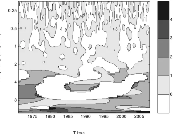
Inﬁgures 10 and 11, the wavelet spectra for the corresponding

standard-ized series is presented. The wavelet spectrum is presented through a contour plot as there are three dimensions involved. The horizontal axis refers to time while the vertical axis refers to frequency. To ease interpretation, the fre-quency is converted to time units (years). The grey scale is for the wavelet spectrum where increasing darkness corresponds to an increasing value and mimics the height in a surface plot. The bold line delimits the statistical sig-nificant area at the usual significance level offive per cent7. All computations

have been done using Matlab.

One can see that both money growth and inﬂation have higher power at

the typical business cycle frequency range, that is, between two and eight

7_{The critical values are based on the results of Torrence and Compo (1998) who have}

(40)

F

r

e

q

u

e

nc

y

(

in

y

e

a

r

s

)

T i m e

1975 1980 1985 1990 1995 2000 2005 0.25

0.5

1

2

4

8

1/4 1/2 1 2 4 8

(41)

F

r

e

q

u

e

n

c

y (

in

ye

a

r

s

)

T i m e

1975 1980 1985 1990 1995 2000 2005 0.25

0.5

1

2

4

8

1/4 1/2 1 2 4 8

(42)

years, as well as at frequencies higher than eight years. For instance, Haug and Dewald (2004), using annual data from 1880 up to 2001 for several countries, also found that lower frequencies are more important in explaining the variance of money growth and inﬂation. Interestingly, there seems to be

an increasing importance of low frequencies in detriment of the remaining ones in both series over time. However, regarding inﬂation, the power is not

statistically signiﬁcant at any frequency at the latter part of the sample. This

reflects theflattening of inflation in the more recent period (see figure 9).

Regarding the relationship between money growth and inﬂation, the wavelet

squared coherency is shown in ﬁgure 12. The wavelet squared coherency is

also presented through a contour plot where increasing darkness corresponds to an increasing value (0_≤ 2₍_{  }₎_≤ ₁_{). Hence, through the inspection of}

the graph one can identify both frequency bands (in the vertical axis) and time intervals (in the horizontal axis) where the series move together. For example, a dark area at the bottom (top) of the graph means strong link at low (high) frequencies whereas a dark area at the left-hand (right-hand) side denotes strong relationship at the beginning (end) of the sample period. Moreover, through such wavelet analysis one can also assess if the strength of the link has increased or decreased over time and across frequencies cap-turing possible varying features in the relationship between the two series in the time-frequency space. The black bold line in the graph delimits the statistical significant area at the usual significance level offive per cent8.

Disregarding higher frequencies, which as mentioned earlier do not re-ceive much attention from the ECB when looking at the money growth and inﬂation relationship, one can see that money growth and inﬂation presented

8_{In this case, as the distribution is not known, the} _ﬁ_{ve per cent signi}_ﬁ_{cance level was}

(43)

F

r

e

q

u

e

nc

y

(

in

y

e

a

r

s

)

T i m e

Note: White area c orresponds to a squared coherency lower than 0.5 with inc reasing darkness corresponding to inc re asing squared coherenc y.

1975 1980 1985 1990 1995 2000 2005 0.25

0.5

1

2

4

8

0.5 0.6 0.7 0.8 0.9

(44)

F

r

e

q

u

e

nc

y

(

in y

e

a

r

s

)

T i m e

Note: White area c orresponds to a negative lead, that is, money growth lags

inflation. Increasing darkness corre sponds to increasing lead. Black area corresponds to a lead higher than four years.

1975 1980 1985 1990 1995 2000 2005 0.25

0.5

1

2

4

8

0 1 2 3 4

(45)

a high and signiﬁcant link at business cycle frequencies only up to the

be-ginning of the 80’s. Hence, it is not surprising that Alveset al. (2007) using

data only from 1980 onwards did notﬁnd any evidence of a link between the

two variables at business cycle frequencies.

Concerning long-term movements, there seems to be a more robust link between money growth and inﬂation in the euro area over the whole period

considered (see also Benati (2005, 2009)). The results are also in line with Jaeger (2003) who found that, using a frequency domain analysis and pre-EMU data since 1961, the relationship between inﬂation and money growth is

stronger at low frequencies than at frequencies associated with business cycle

ﬂuctuations. However, one should note that such link at low frequencies is

stronger during the 90’s up to the beginning of 2000’s while weakening in the more recent period. This may explain why Alveset al. (2007) found evidence

in favour of such link at low frequencies using data up to the beginning of 2000’s which disappears when more recent data is included.

Hence, it seems that money growth has lost information content for track-ing inﬂation medium term movements while for longer term developments

the relationship is not as strong as it was when the euro area was launched. Therefore, one should be cautious about the role played by money growth as an indicator of inﬂation developments in the euro area.

Concerning the lead-lag relationship, the wavelet phase between the two series in the time-frequency space is presented in ﬁgure 13. To ease the

reading of the ﬁgure, the phase is presented in time units (years) and only

the lead time of money growth is discriminated, as this is the focus of the ECB. One can see that, at the business cycle frequency range and at the period where the link is stronger, money growth is leading inﬂation by a lead

(46)

3 years and around 1.5 years, respectively. However, one should note that since the end of the 90’s such characteristic seems to be weakening. This is also in line with the ﬁnding of the recent deterioration of money growth as

leading indicator of inﬂation in the euro area.

So, not only the strength of the relationship between money growth and inﬂation in the euro area seems to have decreased but also the lead time.

These results highlight the importance of a regular assessment of the role of money growth in tracking inﬂation developments in the euro area since

such relationship varies across frequencies and over time. Furthermore, this should also be taken into account in the modelling of the link between money growth and inﬂation.

2.4 Conclusions

In this essay, the link between money growth and inﬂation is assessed through

wavelet analysis. Wavelet analysis constitutes a very promising tool as it represents a reﬁnement in terms of analysis in the sense that both time and

frequency domains are taken into account. The motivation for using wavelet analysis to assess such link comes naturally as there is by now evidence that such relationship varies across frequencies and over time. In particular, the focus is on the euro area as the ECB attributes a privileged role to money growth within the two-pillar monetary policy framework. Hence, a time-frequency view of the relationship between money growth and inﬂation in

the euro area is provided over the last forty years.

It is found that the link between monetary growth and inﬂation in the euro

area presents both frequency and time-varying features. On one hand, the relationship between inﬂation and money growth has been stronger at the

long-term developments than at frequencies associated with business cycle

(47)

frequen-cies over the whole sample period whereas there is only supporting evidence at the business cycle frequency range up to the beginning of the 80’s. In terms of the lead-lag relationship, in time-frequency areas where the link is stronger money growth has shown leading properties. However, there seems to be a deterioration of money growth as leading indicator of inﬂation in the

more recent period. These results highlight the importance of a regular mon-itoring of the usefulness of money growth for tracking medium to long-term developments in euro area inﬂation since such relationship is frequency and

(48)

3 Measuring comovement in the time-frequency

space

9

3.1 Introduction

The measurement of comovement among economic variables is key in several areas of economics and ﬁnance. From the innumerous ﬁelds where such

as-sessment is crucial, one can mention business cycle analysis or asset allocation and risk management, just to name a few.

Traditionally, comovement is assessed in the time domain. The most popular measure of comovement is the well-known correlation coefficient. The contemporaneous correlation coefficient provides in a single number the degree of comovement between the series over the sample period. However, being a synthetic measure it can be rather limited unfolding the relationship between economic variables. For instance, it has been long acknowledged that the degree of comovement may vary over time. To take this feature into account, it has been current practice in the literature to compute a rolling window correlation coefficient or to consider non-overlapping sample periods to evaluate the evolving properties of comovement.

Another strand of literature focus on the frequency domain analysis which is a complementary tool to time domain analysis. In fact, with Fourier analysis, one can obtain additional insights through the study of the rela-tionship between variables at the frequency level (see, for example, A’Hearn and Woitek (2001), Pakko (2004), Breitung and Candelon (2006) and Lem-mens, Croux and DeKimpe (2008)). In this respect, Croux, Forni and Reich-lin (2001) have proposed a spectral-based measure, the dynamic correlation, which allows one to measure the comovement between two series at each in-dividual frequency. This measure, which ranges between₋1and1, is

(49)

tually similar to the contemporaneous correlation between two series in the time domain. However, unlike the correlation coeﬃcient in the time domain, one now obtains a comovement measure that can vary across frequencies. Several applications of the dynamic correlation can be found in recent litera-ture (see, Crone (2005), Rua and Nunes (2005), Camacho, Perez-Quiros and Saiz (2006), Eickmeier and Breitung (2006), Lemmens, Croux and DeKimpe (2007), among others). However, as the dynamic correlation is deﬁned in the

frequency domain it disregards the time dependence of comovement. That is, it provides only a snapshot of the comovement at the frequency level not allowing to capture time-varying features.

Wavelet analysis merges both approaches, in the sense that both time and frequency domains are taken into account. Through wavelet analysis one can assess simultaneously how variables are related at diﬀerent frequen-cies and how such relationship has evolved over time, allowing to capture non-stationary features. This is a distinct and noteworthy aspect as both time- and frequency-varying behaviour cannot be captured using previous approaches. Hence, wavelet analysis constitutes a very promising tool as it represents a reﬁnement in terms of analysis which can provide rich insights

about several economic phenomena (see, for example, the pioneer work of Ramsey and Zhang (1996, 1997) and Ramsey and Lampart (1998a,b)). Re-cent work drawing on wavelets includes, Kim and In (2005) who investigate the relationship between stock returns and inﬂation, Gençay et al. (2005)

and Fernandez (2005) study the Capital Asset Pricing Model, Gallegatiet al.

(2008) and Yogo (2008) resort to wavelets for business cycle analysis, Rua and Nunes (2009) focus on international stock market returns, among others (see, for example, Crowley (2007) for a survey).

(50)

variables move together over time and across frequencies within an uniﬁed

framework. To illustrate the use of such measure, the comovement of growth cycles among the major euro area countries over the last three decades is assessed. Through such empirical application, the usefulness of the pro-posed wavelet-based measure of comovement is highlighted as it allows to unveil both time- and frequency varying features. In fact, it is found that the strength of comovement of growth cycles among the major euro area countries depends on the frequency and has changed over time.

The chapter is organised as follows. In section 3.2, the wavelet-based measure of comovement is presented while in section 3.3, the empirical ap-plication is discussed. Finally, section 3.4 concludes.

3.2 A wavelet-based measure of comovement

The well-known Fourier transform involves the projection of a series onto an orthonormal set of trigononometric components (see, for example, Priestley (1981)). In particular, it uses sine and cosine base functions that have inﬁ

-nite energy (do not fade away) and ﬁnite power (do not change over time).

Hence, the Fourier transform does not allow for any time dependence of the signal and therefore cannot provide any information about the time evolution of its spectral characteristics. To circumvent such limitation it has been sug-gested the so-called short-time or windowed Fourier transform. It consists in applying a short-time window to the signal and performing the Fourier transform within this window as it slides across all the data. A caveat of the windowed Fourier transform is that the window width and thus the time resolution is constant for all frequencies. When a wide range of frequencies is involved, the ﬁxed time window tends to contain a large number of high

(51)

low frequency components. Hence, as the signal is examined under a ﬁxed

time-frequency window with constant intervals in the time and frequency domains, the windowed Fourier transform does not allow an adequate reso-lution for all frequencies. In contrast, the wavelet transform uses local base functions that can be stretched and translated with a ﬂexible resolution in

both frequency and time. In the case of the wavelet transform, the time resolution is intrinsically adjusted to the frequency with the window width narrowing when focusing on high frequencies while widenning when assess-ing low frequencies. As it enables a more ﬂexible approach in time series

analysis, wavelet analysis is seen as a reﬁnement of Fourier analysis.

Mathematically, the wavelet transform decomposes a time series in terms of some elementary functions,_{ }(), which are derived from a time-localized

mother wavelet () by translation and dilation (see, for example, Percival

and Walden (2000)). Wavelets have ﬁnite energy and compact support, that

is, they grow and decay in a limited time period and are deﬁned as

_{ }() = √1



µ

− 

¶

(31)

where  is the time position (translation parameter),  is the scale (di-lation parameter), which is related with the frequency, and _√1

 is a

nor-malization factor to ensure that wavelet transforms are comparable across scales and time series. To be a mother wavelet, (), must fulﬁl certain

criteria: it must have zero mean, R_−∞+∞() = 0; its square integrates to unity, R_−∞+∞2() = 1, which means that () is limited to an inter-val of time; and it should also satisfy the so-called admissibility condition,

0  =R₀+∞|

 ()|2

  +∞ whereb()is the Fourier transform of (),

that is, b() =R_−∞+∞()−__.

The continuous wavelet transform of a time series () with respect to