J. Braz. Soc. Mech. Sci. & Eng. vol.26 número4

Samuel da Silva

and V. Lopes Júnior

Mechanical Engineering Department Av. Brasil, n.º 56, Centro 15385-000 Ilha Solteira, SP. Brazil

samuel@dem.feis.unesp.br vicente@dem.feis.unesp.br

E. Assunção

Electrical Engineering Department Av. Brasil, n.º 56, Centro 15385-000 Ilha Solteira, SP. Brazil

edvaldo@dee.feis.unesp.br

Robust Control to Parametric

Uncertainties in Smart Structures

Using Linear Matrix Inequalities

The study of algorithms for active vibrations control in flexible structures became an area of enormous interest, mainly due to the countless demands of an optimal performance of mechanical systems as aircraft and aerospace structures. Smart structures, formed by a structure base, coupled with piezoelectric actuators and sensor are capable to guarantee the conditions demanded through the application of several types of controllers. This article shows some steps that should be followed in the design of a smart structure. It is discussed: the optimal placement of actuators, the model reduction and the controller design through techniques involving linear matrix inequalities (LMI). It is considered as constraints in LMI: the decay rate, voltage input limitation in the actuators and bounded output peak (output energy). Two controllers robust to parametric variation are designed: the first one considers the actuator in non-optimal location and the second one the actuator is put in an optimal placement. The performance are compared and discussed. The simulations to illustrate the methodology are made with a cantilever beam with bonded piezoelectric actuators.

Keywords: Robust control, LMI, optimal placement of piezoelectric

Introduction

Nowadays it is needed an optimal performance in structural systems in order to obtain lighter and stronger structures, static and dynamic stability and reduction of vibrations caused by external sources (Anthony, 2000). It is possible to use modern techniques of active control associated with intelligent materials to execute these demands. These materials are composed by piezoelectric ceramic (PZT - Lead Zirconate Titanate), commonly used as distributed actuators, and piezoelectric plastic films (PVDF - PolyVinyliDeno Floride), highly indicated for distributed sensors (Clark et al., 1998). The design process of such system encompasses three main phases: structural design; optimal placement of sensor/actuator (PVDF and PZT); and controller design. Consequently, for optimal design purposes, the structure, the sensor/actuator placement and the controller have to be considered simultaneously, (Gonçalves et al., 2002). This article addresses the last two phases. The purpose is aimed to develop an integrated controller design procedure for uncertainties parametric rejection, where the PZTs are bonded in optimal locations.1

The location of sensor/actuator is an extremely important step and affects the signals for the controller. Several authors studied the problem of optimal placement of PZT in the active structural control using different methodologies. The techniques more mentioned in the literature use genetic algorithms (GA) in a procedure of discrete optimization (placement of PZT) and continuous optimization (controller). This technique can find good results, but not necessarily the optimal solution, (Silva and Lopes Jr., 2002). It happens because the objective function involves the controller design, then for each location candidate the controller must be synthesized and evaluated its performance. This technique has many citations in literature, as example, Simpson and Hansen (1996) that used a simple model of an interior aircraft to determine the optimal location of PZT. Furuya and Haftka (1993) found the optimal placement of 8 actuators in a structure with 1507 candidate positions.

Geromel (1989) presented a procedure of convex analysis and global optimization for actuator location using LMI. Oliveira and Geromel (2000) proposed a linear output feedback controller design

Paper accepted November, 2004. Technical Editor: José Roberto de F. Arruda.

with joint selection of sensor and actuator. The approach of the present article uses a different methodology, which was proposed by Panossian et al. (1998) in a practical application and described in details in Gawronski (1998). This proposal involves the computation of the Hf norm systems as the objective function, and it is not

necessary the controller design to evaluate the performance of the candidate location.

Many strategies have been used for control design. For example: Lopes Jr. et al. (2003) presented the control of a beam using pole allocation and classical techniques optimization. Liu and Zhang (2000) showed the control of vibrations in a space truss structure using independent modal space control (IMSC). There are many classical strategies that can be used when the mathematical model is available, for instance pole allocation and optimal control (LQR). However, if the model has uncertainties these methods are not indicated. There are many robust techniques well known in structural control literature, as for instance, Moreira et al. (2001) designed a reduced order Hf controller for an intelligent structure

satellite applications considering dynamic uncertainties requirements.

The objective of this work is to use a recent technique, LMI, to design a robust control considering parametric uncertainties. However, the methodology has forward application for any kind of uncertainties. LMI contributes to overcome many difficulties in control design. In the last decade, LMI has been used to solve many problems that until then was unfeasible through others methodologies, (Boyd et al. 1994).

The major advantage of LMI design is to enable specifications such as stability degree requirements, decay rate, input limitation in the actuators and output peak bounder. It is also possible to assume that the model parameters involve uncertainties. The LMI is a very useful tool for problems with constraints, where the parameters vary in a range of values. Once formulated in terms of LMI a problem can be solved efficiently by convex optimization algorithms, (Gahinet et al., 1995).

is discussed for vibration attenuation of some natural modes. Finally, a numerical application using a cantilever beam with bonded PZT is presented for illustration purpose.

Nomenclature

A = dynamic matrix b = width of the beam B = input matrix C = output matrix d = dielectric constant e = reduction error E = Young’s modulus G = transfer function I = identity matrix

k = number of exogenous inputs K = state-feedback gain

M = generated moment by pair of PZT n = number of modes

N = number of states

p = number of uncertainties parameters P = positive definited matrix

q = modal displacement

q= modal velocity r = number of outputs

R = number of candidate sensor locations s = number of control inputs

S = number of candidate actuator locations t = thickness of the beam

T = placement matrix

u = vector of controlled inputs v = number of vertexes

V = voltage applied by pair of PZT w = vector of disturbance inputs x = state-space vector y = vector of measured outputs Greek Symbols

] = modal damping

Y=natural frequency

V = H placement index

E = bounded output energy

U = maximum value of amplitude on PZT

D = decay rate

P = optimization variable relative to compute Hf norm

: = convex space Subscripts

m = relative to ith mode

r = relative to retained state (modes of nominal model) t = relative to truncated states (modes of residual model) b = relative to structure (beam)

p = relative to PZT

1 = relative to the disturbance input 2 = relative to the controlled input

Structural State-Space Models

A linear differential inclusion (LDI) system, in modal state-space form, considering the matrices with appropriate dimensions and assumed to be known is given by:

x C y

ȍ

t A u

Ǻ

w

Ǻ

x t A

x 1 2  ₍₁₎

where9 is a polytope that is described by a list of vertexes in a convex space.

The modal state-space realization is characterized by the block-diagonal dynamic matrix and the related input and output matrices, (Gawronski, 1998):

>

@

mn m m

mi

C C

C C

Ǻ Ǻ B

Ǻ

Ǻ Ǻ Ǻ Ǻ t A diag t A

2 1

2 2 2

1 2

2

1 2 1

1 1

1

» » » » »

¼ º

« « « « «

¬ ª

» » » » »

¼ º

« « « « «

¬ ª

(2)

where i=1,2,…,n,Ami,B1mi,B2mi and Cmi are 2x2, 2xk, 2xs and rx2

blocks, respectively. These blocks can be obtained in several different forms and also it is possible to convert in another realization through a linear transformation. One possible form to blockAmi(t) can be written by:

» ¼ º «

¬ ª

i i i

i i i mi

A

Z ] Z

Z Z

] ₍₃₎

It is assumed that the natural frequencies vary equally in both, positive and negative, sides, so the natural frequencies corresponding to model obtained by finite element method (FEM) can be taken as nominal parameters. In this paper we considered state feedback and parametric variations only in the low frequency modes (modes of the retained model), described by polytopic LDI (PLDI):

^

r t CoA A

A : :

`

where v is the number of vertexes of the polytopic system. The number of vertexes is given by 2p_{, where p is the number of}

uncertainty parameters. The operatorCo means that the matrixAr,1;

…;Ar,vdefine a convex space.

The state vectorx of the modal coordinates system consists of n independent components,xi, that represent a state of each mode. The

xi (ith state component), related to eq. (3), is defined (Gawronski,

1998):

i mi mi i moi moi

mi i

q q q where q

q

x ] _Z

¿ ¾ ½ ¯ ®

­

(5)

The use of models obtained by FEM demands high number of degrees of freedom (dof). So, the order of the representation is generally very large, causing numeric difficulties. Besides that, the complexity of the controller is model depend, above all, of the order of the plant in study. Therefore, the synthesis of a low order plant is fundamental for a controller success.

A reduced-order model is obtained by truncating the states. Letx and the state (A,B1, B2,C) be partitioned considering the canonical

modal decomposition. From the Jordan canonical form can be obtained:

>

@

¿ ¾ ½ ¯ ® ­

» ¼ º « ¬ ª » ¼ º « ¬ ª ¿ ¾ ½ ¯ ® ­ » ¼ º «

¬ ª ¿ ¾ ½ ¯ ® ­

t r t r

2t 2r

1t 1r

t r

t r

t r

x x C C y

u Ǻ Ǻ w Ǻ Ǻ x x ǹ 0

0 t ǹ x x

(6)

where Ar(t) is given by eq. (4). Nothing about performance

The main problem is to find the order and the retained states that best reproduces the response of the complete system. The choice depends mainly on the definition of the reduction index used. In general, systems norms are used to evaluate the reduction error, (Gawronski, 1998).

Different methods of model reduction through LMI were proposed, for the cases of local and global optimization, using as index the performance systems norms, for instance Assunção et al. (2002) uses Hf norm.

In this work the Hf norm is used as reduction index. The norm

of the ith natural mode (Ami, B2mi,Cmi) can be calculated in different

forms. However, this article uses LMI to the computation of the Hf

norm. Assunção and Teixeira (2001) demonstrate in full detail as to compute this norm. The Hf norm system can be found from the

following optimization problem:

0 µ

0 P

0 µ P

B

PB CC PA P A to subject

µ min G

T T T

! !

» » ¼ º «

« ¬ ª

f

2

2

(7)

This norm also corresponds to the peak gain of frequency response function. The Hf norm system is the same the largest norm of the

modes. The Hf reduction error is defined as:

f r

G -G

e (8)

whereG is the transfer function of the nominal system and Gr is the

transfer function of the nominal model.

Placement of Actuators and Sensors using Hf Norm

The actuator should be placed at a location to excite the desired modes in a most effective way. The optimal placement problem consists of to determine the location of a small set of actuators and sensors such that the Hf norm of the system is the closest possible

of the norm case using large set of actuator and sensor.

The Hf placement index, Vik, evaluates the kth actuator (sensor)

at theith mode. It is defined in relation to all the modes and all the admissible actuators as:

n , 1, i S , 1, k G

ıki ki _f (9)

It is convenient to represent the placement index as a placement matrix:

actuator kth

mode ith

ı ı

ı ı

ı ı

ı ı

ı ı

ı ı

ı ı

ı ı

ȉ

nS nk

n2 n1

iS ik

i2 i1

2S k

2

1S 1k

1 1

ž



» » » » » » » »

¼ º

« « « « « « « «

¬ ª

2 22 1

2 1

(10)

where the kth column consists of indexes of the kth actuator for every mode, and the ith row is a set of the indexes of the ith mode for all actuators.

The actuators with small indices can be removed as the least significant. The largest value indices are optimal placement actuator. Similarly, it is possible to determine the optimal placement of the sensors, (Gawronski, 1998).

State-Feedback Analysis via LMI

The problem to be investigated is the state-feedback control, with the following linear control law:

r

Kx

u (11)

whereK must be found. It is considered to be known all retained states,xr. Therefore it is not necessary to use a dynamic observer. It

is assumed that the reduced model is representative, so, it is not necessary to include any requirements to treat with dynamic uncertainties. The goal of the present paper is to work with only parametric uncertainties described by polytopics.

The system described by eq. (6) can be rewritten in closed-loop:

x_{r r 2r r 1r r} (12)

The system of eq. (12) is quadratically stable if and only if the following LMI is feasible:

0 B Y Y B QA Q A

0 Q

ȉ r T r ȉ

i r, i

r,

!

2 2

(13a,b)

where the symbols >0 and <0 means positive and negative definited, respectively,Ar,i is ith vertex polytopic system,i=1,2,...,v,

vis the number of vertexes and Y=KQ, (Boyd et al., 1994). Assuming that it is desired to bound the output peak energy and thatQ satisfies inequalities (13). Defining the ellipsoid, (Folcher and Ghaoui, 1994):

^

`

H

r T r

r x Q x

x (14)

The ellipsoid is said to be invariant if:

İ t x 0 t İ 0

xr  Ÿ ! r  (15)

wherexr(0), the initial state, is given.

The maximum output energy given a certain initial state is:

:  °¿

° ¾ ½

°¯ ° ® ­

³

f

t A where x

C y x t A x dt y y

max _{r r r r r r}

0

ȉ ₍₁₆₎

Supposing there exists a Lyapunov function V(xr)=xrTQ-1xr such

that,

y y x V 0

Q! r d T (17a,b)

then the condition given by the inequalities (17) is equivalent on LMI to:

v , 1,2,

i

d » » ¼ º «

« ¬ ª

!

0

ǿ

Q C

QC QA Q A

0 Q

r

T r T

i r, i

r, (18a,b)

xr(0)TQ-1xr(0). Then in this case, the output energy is bounded above

xr(0)TQ-1xr(0), whereQ satisfies the LMI:

0 ǿ Q

C

QC B Y Y B QA Q A

0 Q

r

T r T

r T r T

i r, i

r, d

» » ¼ º «

« ¬ ª

!

2

2 (19a,b)

where i=1,2,.., v. Regarding Y as a variable, it can find a state-feedback gain that guarantees output energy less than E by solving the LMI problem:

0 ȕ x

x Q

ȉ r

r _!

» ¼ º «

¬ ª

0 0

(20)

When the initial condition is known, it is also possible to find an upper bound on the norm of the control input, eq. (11). Given Q>0 andY which satisfy the quadratic stabilization condition, inequalities (13), and be limited in the ellipsoid from condition given by eq. (14), the upper bound of the control input can be written as:

2 2 T 1 1

max 1 x

1 0 t 0 t

YQ Y Q x

YQ max

x YQ max u max

H 

t t

O d

Therefore, the constraints

u

d

U

0 I ȡ Y

Y Q 0 Q 0 x

0 x 1

2 T

r

T

r _!

» » ¼ º « « ¬ ª t » » ¼ º «

« ¬ ª

(22)

whereU is the maximum value of amplitude on actuators.

In the same way, it can be possible to impose a decay rate on the closed-loop:

0 B Y Y B QA Q A Q

0 Q

T r r

T i r, i

r,

D

!

2 T 2

2 (23)

Besides, the under largest decay rate can be found solving the generalized eigenvalue problem (GEVP), (Boyd et al. 1993). In summary, the controller design is the result of the following convex optimization problem, consideringU and E known:

(24)

This problem can be solved using interior-point methods, (Gahinet et al., 1995). For each initial condition, the inputu and the outputy assure:

°¯ ° ® ­

t

_ĮĮt_t

ȕe y

ȡe u 0

t (25)

The optimal feedback gain is given by:

1

YQ

K (26)

whereY andQ are solutions from problem given by inequalities (24).

Numerical Application

To verify the proposed methodology, an aluminum cantilever beam, as shown on fig. 1, was considered. The system is discretized by FEM 10 elements (2 dof by node), then the total number of structural dof used was 22. For the cantilever condition the system haveN=40 states. The properties of the beam are given in table 1.

The number of electrical dof changes as a function of the number of PZT considered (2 dof by PZT), (Lopes Jr. et. al., 2000). The PZT size is equal to the discrete finite element size. The properties of PZT, based on material designation PSI-5A-S4 (Piezo Systems, Inc.), are given in table 2.

7

1 2 3

1 2 3

4 5 6

4 5 6 7

8 9 10

8 9 10

Figure 1. Finite element model for a cantilever beam.

Table 1. Beam properties and dimensions.

Length Width Thickness

Dimensions (m)

0.5 0.03 0.005

Density (kg.m-3_{) 2710}

Young’s Modulus (GPa) 70

Table 2. PZT properties and dimensions.

Length Width Thickness

Dimensions (m)

0.05 0.02 0.0015

Young’s Modulus (GPa) 63

Dielectric Constant, d31, (m.V-1) -190e-12

In order to test the proposed optimization method, the optimal location of actuator, a pair of PZT bonded on the beam surface is considered. The objective in this test was to control the first two vibration modes. It was considered to be possible to bond the PZT in all elements. It was, also, considered finding an optimal location to a displacement sensor to state-feedback. The sensor position candidates consider all nodes on vertical direction.

F F

Figure 2. PZT actuators in-phase.

If two PZT elements are fixed on both sides of the beam and the voltage applied on this elements are in-phase, a longitudinal motion is obtained. If the voltages applied on PZT elements are out-of-phase, then it generates moments at the end of the PZT elements, causing lateral motions, as showed at figs. 2 and 3.

M M

Figure 3. PZT actuators out-of-phase.

p 31

s p s p p p p s s s

s p s s 2 s

h d

h h h h h b Ǽ h b Ǽ 6

h h b Ǽ h

V M

¸ ¸ ¸ ¸ ¸

¹ ·

¨ ¨ ¨ ¨ ¨

© §

¸¸ ¹ · ¨¨ © §

¸¸ ¹ · ¨¨ © §

2

8 12 1

(27)

Using eq. (27) and the properties showed on tables 1 and 2, the relationship between the applied voltage and the generated moment is 1836.4/N.m. This means that for a voltage of 110 V, a moment of the order of 0.06 N.m will be generated.

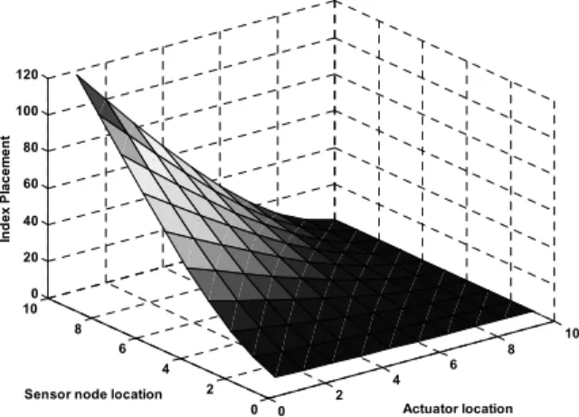
The placement indices computed from eq. (9) of each candidate sensor/actuator for the first two modes are shown in fig. 4. The largest value index is for the PZT actuator bonded in element 1 and sensor on node the free end of the beam (node 10). In our case, for accelerometer, the placement of the sensor in the free end of the beam is not a practical location.

0 2

4 6

8 10

0 2 4 6 8 10

0 20 40 60 80 100 120

Actuator location Sensor node location

In

d

ex P

lacem

ent

Figure 4. Placement indices for control the two first modes versus PZT location and sensor node location.

For the design is considered a disturbance input as showed in fig. 5. In this figure it is also shown the PZT bonded in element 1 and the sensor in a suboptimal configuration.

PZT sensor

disturbance input

Figure 5. Schematic smart structure showing the PZT in a suboptimal location, sensor and disturbance input.

The magnitude plots for transfer function of the complete system and reduced-order model are shown in fig. 6. The transfer functions H1 and H2 are relative with the stace-space realization

(A,B1,C) and (A,B2,C), respectively. A fourth order model is

determined by truncating the system model following the described methodology. The Hf reduction error is about 0.5%. This value was

found through Hf norm problem, given by optimization problem

described in inequality (7). First, it is computed the Hf norm for the

complete model (this value corresponds to the peak gain). In the following the Hf norm relative to the reduced model is found. If the

reduction error, given by eq. (8), is lower that an specified value, it means that the reduced model is representative of the complete system.

A mathematical model provides a map from inputs to responses. The quality of a model depends on how closely its response matches those one of the plant. Since no single fixed model can respond exactly like the true plant, we need, at the very last, a set of maps. The term uncertainty refers to the differences or error between models and reality, and whatever it is used to express error, it is called a representation of uncertainty, (Gonçalves et al., 2002).

Even with accurate models, the simple inclusion of sensors and actuators on the host structure cause change on the dynamic properties of the system. The computation of these uncertainties can be difficult in practical situations, or it has a high computational cost. To solve this problem the model with parametric uncertainties can be quantified by range of parameter values. The parameter uncertainty ranges can be described as parameter box. The controller that satisfies all systems described inside this convex space is said robust to parametric variations. It is enough to solve the optimization problem from eq. (24) for all vertex system simultaneously.

0 100 200 300 400 500 600 700 800 900 1000

-200 -150 -100 -50 0

H

1

-M

a

gni

tude (

d

B

)

0 100 200 300 400 500 600 700 800 900 1000

-150 -100 -50 0

Frequency (Hz)

H

2

- M

a

gni

tude (

d

B

)

Complete Reduced

Complete Reduced

Figure 6. Complete and reduced model magnitude plots for transfer function.

It was considered, in this example, that the system can have a possible variation of r10% in the first and second natural frequencies, so we have 2 uncertainty parameters:

>

@

>

@

1Z 09Z Z 11Z Z Z 09Z Z 11Z

Z min max min max

V1 -1 vertex A min min min min min min min min r, Ÿ » » » » » ¼ º « « « « « ¬ ª Z ] Z Z Z ] Z ] Z Z Z ] 2 2 2 2 2 2 1 1 1 1 1 1 1 0 0 0 0 0 0 0 0 V2 -2 vertex A min min min min max max max max r, Ÿ » » » » » ¼ º « « « « « ¬ ª Z ] Z Z Z ] Z ] Z Z Z ] 2 2 2 2 2 2 1 1 1 1 1 1 2 0 0 0 0 0 0 0 0 V3 -3 vertex A max max max max min min min min r, Ÿ » » » » » ¼ º « « « « « ¬ ª Z ] Z Z Z ] Z ] Z Z Z ] 2 2 2 2 2 2 1 1 1 1 1 1 3 0 0 0 0 0 0 0 0 V4 -4 vertex A max max max max max max max max r, Ÿ » » » » » ¼ º « « « « « ¬ ª Z ] Z Z Z ] Z ] Z Z Z ] 2 2 2 2 2 2 1 1 1 1 1 1 4 0 0 0 0 0 0 0 0

The uncertainties are shown at figure 7. The vertexes of the parameter box are combination of the minimum and maximum values of the parameters of the system. It is supposed that the system can assume any combination of values inside the box.

Z

V1

1 min 2

Z

Z

V3 max 2 2

Z

Z

Z

Figure 7. Parameter box showing the uncertainty combinations.

Figure 8 shows the magnitude plots transfer function for all four open-loop system.

0 25 50 75 100 125 150

-120 -100 -80 -60 -40 -20 Frequency (Hz) H 1 -M a gni tude ( dB

) _{Vertex 1}

Vertex 2 Vertex 3 Vertex 4

Figure 8. Magnitude plots for all four open-loop system.

To test the proposed methodology, firstly we considered a design based on PZT actuator in a particular case non-optimal place position (in this example, in the element 8). The LMI controller was designed considering all vertex system simultaneously. In this case, it was obtained a robust controller that mathematically guarantees the performance specifications in all convex space. The controller is the result of the solution of LMI problem from inequalities (24), whithU= 1, E=2, andxr(0)= [-0.05 0 -0.05 0]T. Next we redesigned

the control law with the PZT actuator in the optimal placement (element 1), and considering the same parametersU, E and xr(0).

During the control, the maximum voltage on PZT was considered as 100 V.

Figure 9 compares the magnitude plots of the controlled and uncontrolled system in the nominal condition for PZT located in element 8 and in the optimal placement. The nominal condition is shown on figure 7.

0 25 50 75 100 125 150

-120 -100 -80 -60 -40 -20 Frequency (Hz) H1 M a gn it u d e (dB) Uncontrolled 1th element 8th element

Figure 9. Magnitude plots for open-loop and controlled system in the nominal condition comparing the PZT placement.

Figure 10 shows the displacement in the time domain for the closed-loop system, considering initial conditionxr(0) for the two

cases considering system in nominal condition.

0 0.1 0.2 0.3 0.4 0.5 0.6 0.7 0.8 0.9 1

-0.05 0 0.05 Mo d e 1

0 0.1 0.2 0.3 0.4 0.5 0.6 0.7 0.8 0.9 1

-0.05 0 0.05 Time (s) M ode 2 1st element 8th element 1st element 8th element

0 25 50 75 100 125 150 -120

-100 -80 -60 -40 -20

V

1

-M

a

gni

tude (

d

B

)

0 25 50 75 100 125 150

-120 -100 -80 -60 -40 -20

Frequency (Hz)

V

2

-Ma

g

n

itu

d

e

(d

B

)

Uncontrolled 1st element 8th element Uncontrolled 1st element 8th element

Figure 11. Magnitude plots for open-loop and controlled system considering the condition of vertex 1 and vertex 2, respectively.

Figures 11 and 12 show the magnitude plots of the controlled and uncontrolled system considering the four extreme conditions (vertexes of the polytopic systems).

0 25 50 75 100 125 150

-120 -100 -80 -60 -40 -20

V

3

-M

a

gni

tude (

d

B

)

0 25 50 75 100 125 150

-120 -100 -80 -60 -40 -20

Frequency (Hz)

V

4

-Ma

g

n

itu

d

e

(d

B

)

Uncontrolled 1st element 8th element

Uncontrolled 1st element 8th element

Figure 12. Magnitude plots for open-loop and controlled system considering the condition of vertex 3 and vertex 4, respectively.

Comparing the figs. 9 until 12 it is possible to observe (in this case) that the effort of the controller with PZT bonded in the 8th

element is larger than in the optimal placement. Besides, the attenuation of the interested modes is bigger when the PZT is in an optimal placement. As a result of the active damping the peaks at the resonance of the controlled modes are reduced.

Conclusions

The main theoretical contribution of this research work was to propose and to motivate the use of LMI in the structural control community.

First was showed a brief review of structural state-space model in modal coordinates and a reduction model. After this, a strategy

for placement of actuators and sensors using Hf norm was

presented. This technique of optimal location could be implemented using others norms, for instance, H2 norm. In the following a LMI

controller was proposed for amplitude attenuation of some modes. To illustrate this procedure was considered the control of a cantilever beam modeled by FEM. In this particular example the state-space model had 40 states. After the reduction procedure it was

obtained a model with 4 states that well represented the complete dynamic system. Moreover, we designed a LMI controller robust to parametric variations and compared the amplitude attenuation for PZT in optimal and non-optimal location.

The authors are encouraged by the results obtained and it seems that the methodology developed can be extended to other practical systems, for example, smart plates and space truss structures. An experimental investigation is being implemented in the Vibration Laboratory of UNESP/Ilha Solteira to check the results obtained in the numerical simulations.

Acknowledgements

The authors acknowledge the support of the Research Foundation of the State of São Paulo (FAPESP-Brazil) and of the National Council of Scientific and Technological Development (CNPq-Brazil). The authors would like to thank the Associate Editor and the reviewers for their valuable comments.

References

Anthony, D. K., 2000, “Robust Optimal Design Using Passive and Active Methods of Vibration Control”, Ph. D. Thesis, Faculty of Engineering And Applied Science, Institute of Sound And Vibration Research, University of Southampton, 267 p.

Assunção, E. and Teixeira, M. C. M, 2001, “Projeto de Sistema de Controle Via LMIs usando o MATLAB”, APLICON, Escola Brasileira de Aplicações em Dinâmica e Controle. USP – São Carlos – SP.

Assunção, E., Marchesi, H. F.,Teixeira, M. C. M. and Peres, P. L. D., 2002, “Otimização Global Rápida para o Problema de Redução Hf de Modelos”, XIV Congresso Brasileiro de Automática, Natal – RN.

Boyd, S., Balakrishnan, V., Feron, E. and El Ghaoui, L, 1993, “Control System Analysis and Synthesis via Linear Matrix Inequalities”, Proceeding of American Control Conference, pp. 2147-2154.

Boyd, S., Balakrishnan, V., Feron, E. and El Ghaoui, L, 1994, Linear Matrix Inequalities in Systems and Control Theory, SIAM Studies in Applied Mathematics, USA.

Brennan, M. J., Day, M. J., Elliot, S. J. e Pinnington, R. J., 1994, “Piezoelectric Actuators and Sensors”, Proceedings of the IUTAM Symposium of the Active Control of Vibration - Bath, pp 263-274;

Clark, R.L., Saunders, W.R., and Gibbs, G.P., 1998, Adaptible Structures: Dynamics and Control, John Wiley & Sons, Inc.

Folcher, J. P. and El Ghaoui, L., 1994, “State-Feedback Design via Linear Matrix Inequalities Application to a Benchmark Problem”, IEEE ISBN 0-7803-1872-2, pp. 1217-1222.

Furuya, H. e Haftka, R. T., 1993. “Locating Actuators for Vibration Supression on Space Trusses by Genetic Algorithms”, Structures and Control Optimization, ASME 1993, pp. 1-11.

Gahinet., P., Nemirovski, A.,. Laub, A. J. and Chiliali, M., 1995, LMI Control Toolbox User’s Guide, The Mathworks Inc., Natick, MA, USA.

Gawronski, W., W., 1998, Dynamics and Control of Structures: A Modal Approach, 1.ed. New York: Springer Verlag.

Geromel, J. C., 1989, “Convex Analysis and Global Optimization of Joint Actuator Location and Control Problems”, IEEE Trans. On Automatic Control, 34 (7), pp. 711-720.

Geromel, J. C., Peres, P. L. D. and Bernussou, J., 1991, “On a Convex Parameter Space Method for Linear Control Design of Uncertain Systems”, SIAM J. Control and Optimization, 29 (2), pp. 381-402.

Gonçalves, P. J. P., Lopes Jr., V., and Assunção, E., 2002, “H2 and Hf

Norm Control of Intelligent Structures using LMI Techniques”, Proceeding of ISMA 26 - International Conference on Noise and Vibration Engineering, Leuven, Belgium.

Liu, F. and Zhang, L., 2000, “Modal-Space Control of Flexible Intelligent Truss Structures via Modal Filters”, Proceeding of IMAC -International Modal Analysis Conference, pp. 187-193.

Lopes Jr., V., Steffen Jr., V., and Inman, D .J., 2000, “Optimal Design of Smart Structures Using Bonded Piezoelectric for Vibration Control”, Proceeding of ISMA 25 – International Conference on Noise and Vibration Engineering, Leuven, Belgium.

Moreira, F.J.O., Arruda, J.R.F., and Inman, D.J., 2001, "Design of a reduced Order Hinfinity Controller for Smart Struture Satelite Applications", Philosophical Transactions of the Royal Society A, Mathematical, Physical and Engineering Sciences, ISSN 1364-503X, Volume 359, No. 1788, pp. 2251-2270.

Silva, S. and Lopes Jr., V., 2002, “Técnicas de Controle Ótimo para Supressão de Vibração Utilizando Sensores e Atuadores Piezelétricos”, II Congresso Nacional de Engenharia Mecânica - CONEM 2002, João Pessoa-PB.

Simpson, M. T. and Hansen, C. H., 1996, “Use of Genetic Algorithms to Optimize Vibration Actuator Placement for Active Control of Harmonic Interior Noise in a Cylinder with floor structure”, Noise Control Engineering Journal, pp. 169-184.

Oliveira, M. C. and Geromel, J. C., 2000, “Linear Output Feedback Controller Design with Joint Selection of Sensors and Actuators”, IEEE Trans. On Automatic Control, 45(12), pp. 2412-2419.