ISSN 0104-6632 Printed in Brazil
www.abeq.org.br/bjche
Vol. 30, No. 02, pp. 323 - 335, April - June, 2013
Brazilian Journal
of Chemical
Engineering
VERIFICATION AND VALIDATION IN CFD FOR A
FREE-SURFACE GAS-LIQUID FLOW IN
CHANNELS
C. Soares
1*, D. Noriler
4, M. R. Wolf Maciel
2, A. A. C. Barros
3and H. F. Meier
41
Laboratório de Controle de Processos (LCP), Departamento de Engenharia Química e Engenharia de Alimentos (EQA), Universidade Federal de Santa Catarina (UFSC),
C. P. 476, CEP: 88040-900, Florianópolis - SC, Brasil. E-mail: [email protected]
2Laboratório de Desenvolvimento de Processos de Separação (LDPS), Faculdade de Engenharia Química,
Universidade Estadual de Campinas (UNICAMP), C. P. 6066, CEP: 13081-970, Campinas - SP, Brasil. E-mail: [email protected]
3Laboratório de Desenvolvimento de Processos (LDP), Departamento de Engenharia Química,
Universidade Regional de Blumenau (FURB), Campus II, CEP: 89030-000, Blumenau - SC, Brasil. E-mail: [email protected]
4
Laboratório de Fluidodinâmica Computacional (LFC), Departamento de Engenharia Química, Universidade Regional de Blumenau (FURB), Campus II, CEP: 89030-000, Blumenau - SC, Brasil.
E-mail: [email protected]
(Submitted: February 28, 2012 ; Revised: April 3, 2012 ; Accepted: July 31, 2012)
Abstract - This work deals with experimental and numerical studies of a 3-D transient free-surface two-phase flow in a bench-scale channel flow. The aim was to determine how well the homogeneous model can predict the fluid dynamics behavior and to validate the model. The model was validated with experimental data acquired for two hydrodynamic situations. The mathematical model was based on the mass conservation equations for liquid and gas phases and on the momentum conservation equation for the mixture, assuming interpenetrating, continuum and homogeneous hypotheses. Turbulence has been considered for the mixture through the standard k-ε model. The numerical methods were the finite volume method with pressure-velocity coupling and a numerical grid on a generalized Cartesian coordinate system. Good qualitative and quantitative agreements were found for both cases, making the prediction of the fluid dynamics behavior quite robust. Keywords: Computational fluid dynamics; Multiphase flow; Homogeneous model.
INTRODUCTION
According to Versteeg and Malalasekera (1995), “CFD is the analysis of systems involving fluid flow, heat transfer and associated phenomena such as chemical reaction by means of computer-based simulation.” Over the past two decades, the world saw an increase of this technique in the prediction of internal and external flows (Versteeg and Malalasekera, 1995). Although the history of compu-tational fluid dynamics is relatively short, the progress using CFD has been enormous. This has contributed
Besides, CFD allows engineers to propose and develop alternative designs with low cost. In regions or processes where measurements are either difficult or dangerous, like in nuclear reactors, CFD makes it possible to obtain comprehensive and important information on the flow field. It is evident that models based on CFD techniques have been significantly enhanced and calculation speeds have greatly increased in the last ten years. Thus, the use of CFD to simulate hydrodynamics in complex flows has increased drastically and its advantages, as well as its limitations, have been identified (Sundaresan, 2000; Gunzburger and Nicolaides, 1993). This does not mean that experimental tests are not necessary; however, the number of tests can be reduced. Physical experiments are strongly recommended as a comple-mentation to the numerical modeling since they are necessary to verify and to validate numerical solutions.
Many studies presented and reported in the literature have indicated that success in the design of a process and the efficiency of the scale-up depends on the complete understanding of multiphase fluid dynamics. Based on this, in recent years, consider-able effort has been directed towards fundamental fluid dynamics modeling of two-phase flows with the aim of using these models as tools in the design process (Alizadehdakhel et al., 2009; Kakaç et al., 2009; Jovanović et al., 2008; Liu and Wang, 2008; Noriler et al., 2008; Podowski, 2008).
Until recently, the application of computational fluid dynamics as a powerful tool was highly restricted in industry due to the limitation associated with the need for high performance computation. On the other hand, as mentioned, the use of CFD codes will not eliminate the need for experimental testing. However, it will enhance the effectiveness of testing. Despite the increase in the use of this tool, it is necessary to have efficient ways to evaluate the results obtained. Verification and validation are essential methods to be used during the development of mathematical models and simulation of physical processes using CFD techniques. While verification deals with numerical characteristics of the problem, such as approximation schemes, numerical grids, convergence rate, among others, validation deals with the capability of the model to predict the physical characteristics of the situation. According to Oberkampf and Trucano (2002), “verification will be seen to be rooted in issues of continuum and discrete mathematics and in the accuracy and correctness of complex logical structures (computer codes)”. On the other hand, validation is deeply rooted in the question of how formal constructs of nature (mathematical models) can be tested by physical
observation (Oberkampf and Trucano, 2002). Based on these aspects, it is necessary to carry out research that involves complex numerical models in relatively simple geometries to promote the validation of a methodology for multiphase flow and to allow the advance of research in real situations in the chemical engineering field.
The application of CFD involves the mathematical modeling and numerical solution of the governing equations for fluid flow, with or without heat and mass transfer, radiation, and chemical reaction. According to the VOF method, all these equations are numerically solved at thousands of discrete points (computational grid) in a well-defined physical domain that represents the real problem. When the process involves the flow of more than one phase, one approach is to model this process by solving one set of Navier-Stokes equations for each phase. This modeling technique, called the two-fluid, multi-fluid, or Eulerian-Eulerian technique, assumes that the phases are interpenetrating continuous media. There are two basic multi-phase models available, the heterogeneous model and the homogeneous model. The latter, being a simplification of the multi-fluid model, assumes that the velocity is the same for all phases (Hansen et al., 2002). The advantage of this model is that it reduces the number of non-linear algebraic equations in the computational domain, even representing adequately the behavior of gas-liquid flow.
In this context, this study involves numerical and experimental studies of a transient, three-dimensional and multiphase flow in a channel flow, on a bench scale. In recent work in the literature, Murzyn and Bélorgey (2005) measured turbulence length scales in wave/current interaction free-surface flows. Sarker and Rhodes (2004) used the simple geometry of a rectangular broad-crested weir to test commercial CFD software.
The aim of this investigation is to determine how well the homogeneous model can represent the physical situation of free-surface two-phase flow, in order to assess its potential to model more complex systems involving gas-liquid flow, common in processes such as distillation, absorption, bubble columns, and other important unit operations in chemical engineering.
EXPERIMENTAL DETAILS
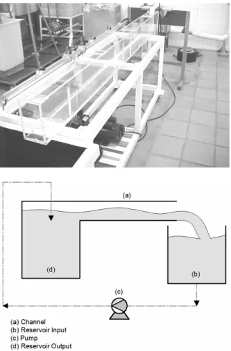
the top, as shown in Figure 1. The water from the tank is pumped through the pipe, enters the reservoir, passes through the flume and returns to the tank. The channel is 2.472 m long, 0.122 m wide, and 0.222 m deep, with a transparent structure made of acrylic material (0.011 m thick) to facilitate visualization of the flow. The reservoir is 5 m in height, 3 m wide, and 0.122 m deep. A sketch of the reservoir is presented in Figure 1.
Figure 1: Experimental apparatus for evaluating the model prediction and a sketch of the reservoir connected to the channel.
The experimental apparatus allows a rectangular obstacle (weir) of 10 mm × 70 mm to be inserted in the centre of the flume, which disturbs the flow and causes the reverse wave phenomenon, i.e., a large portion of the water returns to the inlet section.
Measurements of the liquid height and the operating time, along with a film of the flow dynamics, were the experimental information obtained in order to characterize and validate the numerical model of the air-water flow.
The feed flow was supplied by a tube 40 mm in diameter with an inlet area of approximately 1.2566×10⁻³
m2 (Ainlet); the feed flow rate in all experiments (water with fl,inlet = 1) was kept constant at 2.116×10⁻³
m3/s (Qinlet).
Two configurations were used in this study: in the first situation, lateral profiles of the liquid height were measured at different vertical positions in the flume; in the second situation the profiles were obtained with an obstacle located in the centre of the flume. In both situations a scale was used to determine the height of the liquid in the flume for two hydrodynamic situations. Free-surface profiles at intervals of 10, 20 and 30 mm were obtained along the flume. During the experimental procedure, the water was maintained at room temperature and all experiments carried out at this temperature. It should be mentioned that the flow rates were considered constant at 127 L/min in the validation study.
FLUID DYNAMIC MODEL
Conservative Governing Equations – Homogeneous Model
The homogeneous multi-phase model is used to predict gas-liquid flows. This is the simplest model within the continuous fields approach and, according to Equation (1), it assumes that the velocity for each phase is the same as the mixture velocity (Arastoopour, 1978; Hansen et al., 2002):
p i = , 1 i N≤ ≤
v v , (1)
where i and Np are phase i and the total number of phases, respectively, and v is the velocity vector of the mixture.
The volume fractions are still assumed to be distinct. Hence, the individual phase continuity equations can be solved to determine the volume fractions, but the individual transport equations can be summed over all phases to give a single transport equation for a generic scalar transport equation (Tremante et al., 2002). In the mass conservation equations for gas and liquid phases, the second and third-order correlations that appear as a consequence of the application of time-averaged and Reynolds decomposition are neglected through a simple order-of-magnitude analysis.
Mass Conservation Equation:
• Gas Phase,
( )
g g(
)
g gρ f
ρ f 0
t ∂
+ ⋅ =
∂ ∇ v ; (2)
• Liquid Phase,
( )
l l(
)
l l
f
f 0
t ∂ ρ
+ ⋅ ρ =
∂ ∇ v . (3)
Momentum Conservation Equation:
( )
(
)
(
)
p t
∂ ρ + ⋅ ρ = − − ⋅ + ρ ′ ′ + ρ ∂
v
vv v v g
∇ ∇ ∇ τ . (4)
In Equations (2), (3) and (4), ρ is the density of the mixture of air and water weighted by the use of the volume fraction of the phases, t is time, v is the velocity vector of the mixture, ρg, ρl, fg and fl are the densities and the volume fractions for the mixture of gas and liquid, respectively, g is the acceleration of gravity, p is the thermodynamic pressure, τ is the
viscous stress and ρv v' ' is the Reynolds tensor. The velocity vector (v), density (ρ) and viscosity (μ) of the mixture are given by Equations (5)-(7):
g l
= =
v v v , (5)
p N i i i 1 f =
ρ =
∑
ρ , (6)p N i i i 1 f =
μ =
∑
μ , (7)under the following restriction for the volume fractions constraint (Equation (8)):
p N i i 1 f 1 = =
∑
. (8)Turbulence Model
The well-known single-phase standard k-ε turbulence model (Launder and Spalding, 1974) was used to model the turbulence phenomena in the gas-liquid flow. It is based on the Boussinesq hypothesis,
in addition to homogeneity hypothesis, which expresses the Reynolds stress for the mixture of gas and liquid through Equation (9):
(
)
( )
Tt t
2 2
3 3
⎡ ⎤
′ ′
−ρ = − ρκ − μ ⋅ + μ ∇ + ∇
⎣ ⎦
v v δ ∇ v δ v v , (9)
where κ is the bulk viscosity, δ is the identity tensor, and μt is the eddy viscosity. For an incompressible flow, Equation (10) demonstrates that:
(
)
t
2 2
0
3 3
− ρκ − μδ ∇⋅v δ= . (10)
The eddy viscosity for the mixture of gas and liquid is defined according to Equation (11):
2
t k
Cμ
μ = ρ
ε . (11)
From Equation (11), the standard k-ε model requires two transport equations (partial differential equations or PDEs): one for the turbulent kinetic energy (k) and one for the dissipation rate of turbulent kinetic energy (ε):
( )
(
)
tk
k
k k G
t
⎡⎛ ⎞ ⎤
∂ ρ + ⋅ ρ = ⋅ μ +μ ∇ + − ρε
⎢⎜⎜ ⎟⎟ ⎥
∂ ∇ v ∇ ⎢⎣⎝ σ ⎠ ⎥⎦ (12)
and
( )
(
)
(
)
t 1 2 tC G C
k ε
⎡⎛ ⎞ ⎤
∂ ρε + ⋅ ρε = ⋅ μ +μ ∇ε ⎢⎜⎜ ⎟⎟ ⎥
∂ ⎢⎣⎝ σ ⎠ ⎥⎦
ε
+ − ρε
v
∇ ∇
, (13)
where G represents the generation of turbulent kinetic energy and can be defined by Equation (14). The scalar product of two tensors
( )
: in Equation (14) is known as a double dot product and has a complete definition in the tensor notation.( )
T effG= μ ∇v:⎡⎣∇ + ∇v v ⎤⎦, (14)
with the effective viscosity expressed by Equation (15):
eff t
μ = μ + μ . (15)
by comprehensive data fitting for a wide range of turbulent flows.
Geometry and Boundary Conditions
To solve the continuity and momentum equations, appropriate boundary conditions must be specified at all boundaries. Intuition and experience guided us in specifying the boundary conditions. Also, due to the elliptical characteristics of the partial differential equations of the model, from a mathematical point of view, boundary conditions at all frontiers of the physical domain are necessary. In this case, the
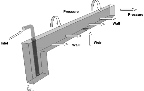
velocity field is adopted as uniform and normal to the surface in the inlet, with non-slip conditions for all the walls, and the pressure conditions are adopted in the outlet and exposure regions. Figure 2 shows a schematic diagram of the physical domain for the two cases studied (without and with weir), and all boundary conditions adopted. Table 1 presents its mathematical form for the two-phase flow.
Water and air at room temperature and atmospheric pressure were the fluids used in the simulation. Initially all of the physical domain is filled with air, representing the initial condition of the phenomenon. Inlet Pressure Weir Pressure Wall Wall Inlet Pressure Weir Pressure Wall Wall
Figure 2: View of the geometry used in the numerical simulation.
Table 1: Mathematical form of the boundary conditions.
Phase Boundary
Conditions Mixture Liquid Gas
Inlet inlet x inlet inlet Q v A
= vy inlet=0 vz inlet=0
(
)
2inlet x inlet
3
k I v
2
= ⋅
(
)
3 2 inlet inlet inlet k D ε = l l,inletf =f fg= −1 fl,inlet
Outlet
y x
outlet outlet outlet outlet
v
v k
0
∂
∂ = =∂ =∂ε =
∂η ∂η ∂η ∂η
ref
p=p
l outlet f 0 ∂ = ∂η g outlet f 0 ∂ = ∂η
Wall x wall y wall wall wall
v v k 0
y ∂ε = = = = ∂ l wall f 0 ∂ = ∂ζ g wall f 0 ∂ = ∂ζ η is the direction orthogonal to the outlet.
Numerical Grid
The pre-processor BUILD of the CFX 4.4 commercial CFD code, from ANSYS Inc., was used to generate the numerical grid for the geometry of the computational domain. The total number of grid cells within the computational domain was 144,079, which presents an independence of the numerical solutions on the grid concentration. Figure 3 shows the numerical grid adopted for the CFD studies.
NUMERICAL METHODS AND SOLUTION STRATEGIES
The foregoing mathematical model has been incorporated for general use into the commercial CFD code CFX 4.4, from ANSYS Inc., which is a finite volume solver, using body-fitted grids, subjected also to the verification studies described herein. Discretization of the equations over the grid is carried out using a finite volume method, where the physical domain is mapped in a rectangular compu-tational space.
Velocity vector equations (momentum conserva-tion) are treated as scalar equations and all scalar variables are discretized and calculated at the cell centre. An improved Rhie-Chow interpolation
algorithm (Rhie and Chow, 1983) was employed for determination of velocities required at the cell faces. Diffusion coefficients, effective viscosities and other transport variables are calculated and stored at the cell faces. The pressure-velocity coupling is obtained using the SIMPLEC algorithm (Van Doormal and Raithby, 1984). For the convective terms Higher-Order Upwind was used. The transient equations were solved for about 30 s until steady-state was reached. For the time term, implicit first-order backward time differencing was used. Details regarding the numerical method can be found in Versteeg and Malalasekera (1995).
When calculating the two-phase flow, it is possible that the interface becomes smeared out, owing to numerical diffusion in the void fraction. The surface-sharpening algorithm used in this study defines the surface as being where the volume fraction is equal to fifty percent of each phase in the two-phase flow. Thus, the algorithm identifies fluid on the side of the interface with less than the fifty percent in volume fraction and moves it to the other side of the interface to conserve the mass in the volume. The surface-sharpening algorithm was used based on preliminary tests obtained in a different geometry. Details regarding this algorithm and its influence on the numerical solution can be found in Soares et al. (2002) and in Hansen et al. (2002).
(a) (b)
(c)
RESULTS AND DISCUSSION
The aim of the numerical simulations was to verify and validate the mathematical modeling in the CFD through comparisons with experimental data. Analysis of the two-phase flow dynamics was carried out, seeking a better understanding of the main fluid dynamics phenomena that are responsible for the heat, mass and momentum transfer between phases.
Verification of the Numerical Methods and the CFD Code
The verification study of numerical methods and the CFD code was carried out with a view to improving the performance of the numerical experi-ments, in terms of the convergence and stability of the numerical solutions.
Non-dependence of the solution on the numerical grid was reached at around 144,000 cells, and with the concentration of the grid close to the inlet / outlet section and close to the inlet, according to Figure 3.
A higher-order upwind interpolation scheme was also used, coupled with the Rhie-Chow algorithm, to avoid numerical diffusion and numerical instabilities, with high convergence rates in all numerical experiments.
Validation of the Mathematical Model
The model was validated against measurements taken based on an air-water system at atmospheric
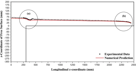
pressure. Profiles related to the liquid height during the flow were selected at several points along the experimental apparatus, for both cases, to be compared with the numerical data. The y-coordinate in the figures represents the distance measured in the flume.
Table 2 shows the experimental data, numerical prediction and absolute and relative error for each case: without and with the obstacle, respectively.
Figures 4 and 5 show the measured and predicted longitudinal free-surface profiles, and the similarity between the experimental and numerical results for both situations demonstrates the accuracy to which the homogeneous model was able to reproduce the real behavior of the flow inside the channel, mainly in the regions represented by (a) and (b) in Figure 4 and (a), (b) and (c) in Figure 5.
A good qualitative agreement between the experimental and numerical predictions can also be observed in Figure 6, which presents a comparison between an image of the wave generated inside the channel flow due to the obstacle and the isocurve obtained numerically for the same physical situation.
Based on the results obtained, it is possible to conclude that the mathematical model can be considered validated, since it is able to represent the real dynamics of the flow and, consequently, it can be applied to predict the fluid dynamics in situations involving free-surface flows, due to the general formulation employed during the development of the mathematical modeling.
Table 2: Experimental and numerical data.
z-Coordinate of Free Surface (mm) Error Longitudinal
y-Coordinate (mm) Experimental Data Numerical Prediction Absolute Relative (%) without
obstacle
with obstacle
without obstacle
with obstacle
without obstacle
with obstacle
without obstacle
with obstacle
0 71 77 64.2 69.7 6.8 7.3 10.6 10.5
90 69 75 63.3 68.9 5.7 6.1 9.0 8.8
180 68 72 61.9 67.5 6.1 4.5 9.8 6.7
360 53 62 49.0 57.9 4.0 4.1 8.2 7.1
540 56 63 48.3 57.5 7.7 5.5 15.9 9.6
730 54 62 47.2 57.1 6.8 4.9 14.4 8.6
910 53 61 46.8 56.7 6.2 4.3 13.2 7.6
1090 51 61 46.0 56.2 5.0 4.8 10.9 8.5
1270 50 59 45.0 55.6 5.0 3.4 11.1 6.1
1450 49 32 43.7 35 5.3 -3.0 12.1 -8.6
1660 46 28 42.1 33.4 3.9 -5.4 9.3 -16.2
1810 45 38 41.6 34.9 3.4 3.1 8.2 8.9
1990 43 41 40.2 36.2 1.4 4.8 3.5 13.3
2160 41 41 37.7 36.8 3.3 4.2 8.8 11.4
2340 36 35 33.9 33.1 2.1 1.9 6.2 5.7
0 250 500 750 1000 1250 1500 1750 2000 2250 2500 -300
-275 -250 -225 -200 -175 -150 -125 -100 -75 -50 -25 0 25 50 75 100 125 150 175 200
(b) (a)
Experimental Data Numerical Prediction
z-Co
or
di
n
a
te
of
Fr
ee
Sur
fa
ce
(
mm)
Longitudinal y-coordinate (mm)
Figure 4: Longitudinal free-surface profiles (without obstacle).
0 250 500 750 1000 1250 1500 1750 2000 2250 2500 -300
-275 -250 -225 -200 -175 -150 -125 -100 -75 -50 -25 0 25 50 75 100 125 150 175 200
(c) (b)
(a)
Experimental Data Numerical Prediction
z-Coor
di
nat
e of
F
re
e Sur
fa
ce
(mm)
Longitudinal y-Coordinate (mm)
Figure 5: Longitudinal free-surface profiles (with obstacle).
Scientific Visualization of the Two-Phase Flow
Scientific visualization of the flow through a CFD postprocessor is a very common tool in CFD studies, since it permits the inspection of fluid dynamics phenomena at a level of detail that the macroscopic
point of view does not allow.
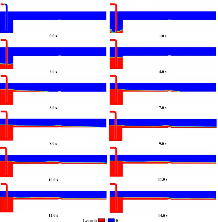
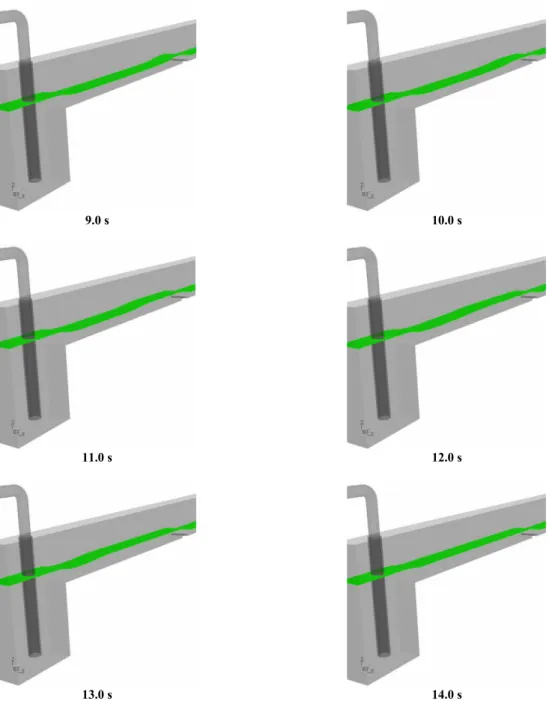
Tests with the surface-sharpening algorithm for smoothing of free surfaces were carried out and good effects were produced for the development of the gas-liquid flow. Figure 7 illustrates the fluid dynamic behavior obtained by the solution of the model.
0.0 s 1.0 s
2.0 s 4.0 s
6.0 s 7.0 s
8.0 s 9.0 s
10.0 s 11.0 s
12.0 s 14.0 s
Legend: 1 0
Figure 7 also shows that 7 seconds after the beginning of the flow a wave appears close to the obstacle, and the formation of a reverse wave begins close to the liquid surface, which promotes the return of the liquid to the inlet of the channel until the level of the liquid becomes uniform. This behavior can be observed in Figures 7 and 8 at between 9 and 12 seconds. This corroborates the conclusion regarding
the ability of the homogeneous model to predict the real dynamics of the flow, and the validation of the mathematical model.
Figure 9 shows that the modeled dynamics of the reservoir filling up is very similar to the experiments, showing again the high performance of the numerical homogeneous model to represent the gas-liquid flow inside the channel flow.
9.0 s 10.0 s
11.0 s 12.0 s
13.0 s 14.0 s
0.05 s 0.25 s
0.50 s 0.75 s
1.00 s 1.25 s
1.50 s 2.00 s
4.00 s 6.00 s
CONCLUSIONS
An experimental and numerical study of a 3-D transient free-surface two-phase flow (water-air) in a bench scale channel flow was carried out aiming to determine how well the homogeneous model can predict the free-surface fluid dynamic behavior inside the free surface channel, and to validate the model for application to a wide range of important flows in chemical engineering.
The validation of the mathematical model shows the applicability and simplicity of the homogeneous model in modeling and representing the main fluid dynamics in free-surface flows. The advantage of this model is that it reduces the number of non-linear algebraic equations in the computational domain and continues to represent adequately the behavior of the gas-liquid flow, when compared to the heterogene-ous model, which is much more robust but requires a large number of constitutive equations.
According to the results obtained, the mathemati-cal model based on the homogeneous model was able to represent the physical situation, showing an excellent agreement between simulated and experimental profiles of the volume fraction and the ability to represent adequately the flow dynamics and its main phenomenological characteristics. The proposed model also accurately predicted the wave generated when an obstacle was included, which is an important feature.
Furthermore, the CFD techniques used in this study represent a powerful tool to analyze fluid dynamics phenomena in a channel flow, and can be used in advanced studies of important fields of chemical engineering.
NOMENCLATURE
Latin Letters
Ainlet inletarea m2
C1, C2, Cµ
constant of the standard k-ε turbulence model
f volume fraction
G generation of turbulent kinetic energy
(J/m3)/s g gravitational acceleration
vector
m/s2
I turbulence intensity
k turbulent kinetic energy m2/s2 Np total number of phases
p pressure Pa
Qinlet feed flow rate L/min
t time s
v velocity vector m/s
Greek Letters
κ bulk viscosity kg/m·s
ε dissipation rate of turbulent energy
m2/s3 ρ effective density of the
mixture
kg/m3 δ identity tensor
η direction orthogonal to the outlet
ζ direction orthogonal to the wall
σk, σε
constant of the standard k-ε turbulence model
µ viscosity kg/m·s
µeff effective viscosity kg/m·s
µt eddy viscosity kg/m·s
Subscripts
g gas phase
i phase
l liquid phase
REFERENCES
Arastoopour, H., Hydrodynamic analysis of solids transport. Ph.D. Thesis, Illinois Institute of Technology, Illinois, Chicago (1978).
Alizadehdakhel, A., Rahimi, M., Sanjari, J. and Alsairafi, A. A., CFD and artificial neural network modeling of two-phase flow pressure drop. International Communications in Heat and Mass Transfer, 36, (8), p. 850-856 (2009).
Jovanović, R., Cvetinović, D., Stefanović, P. and Swiatkowski, B., Turbulent two-phase flow modeling of air-coal mixture channels with single blade turbulators. FME Transactions, 36, p. 67-74 (2008).
Gunzburger, M. D. and Nicolaides, R. A., Incom-pressible Computational Fluid Dynamics: Trends and Advances. Cambridge University Press, Cambridge (1993).
Hansen, K. G., Madsen, J., Trinh, C. M., Ibsen, C. H., Solberg, T. and Hjertager, B. H. A., Computational and Experimental Study of the Internal Flow in a Scaled Pressure-Swirl Atomizer. ILASS-Europe, Zaragoza (2002).
instabilities in convective in-tube boiling horizontal systems. J. of Thermal Science and Technology, 29, 1, p. 107-116 (2009).
Launder, B. E. and Spalding, D. B., The numerical computation of turbulent flows. Comp. Meth. Applied Mech. Eng., 3, p. 269-289 (1974).
Liu, D. and Wang, S., Flow pattern and pressure drop of upward two-phase flow in vertical capillaries. Ind. Eng. Chem. Res., 47, p. 243-255 (2008).
Marquardt, W., Trends in computer-aided process modelling. Computers and Chemical Engineering, 20, p. 591-609 (1996).
Murzyn, F. and Bélorgey, M., Wave influence on turbulence length scales in free surface channel flows. Experimental Thermal and Fluid Science, 29, p.179-187 (2004).
Noriler, D. Meier, H. F. Barros, A. A. C. and Wolf Maciel, M. R., Thermal Fluid dynamics analysis of gas–liquid flow on a distillation sieve tray. Chemical Engineering Journal, 136, 1, p. 133-143 (2008).
Oberkampf, W. L. and Trucano, T. G., Verification and validation in computational fluid dynamics. Progress in Aerospace Sciences, 38, p. 209-272 (2002).
Orszag, S. A. and Staroselsky, I., CFD: Progress and problems. Computer Physics Communications, 127, p. 165-171 (2000).
Podowski, M. Z., Multidimensional modeling of two-phase flow and heat transfer. International Journal of Numerical Methods for Heat & Fluid Flow, v. 18, n. 3/4, pp. 491-513 (2008).
Rhie, C. M. and Chow, W. L., Numerical study of the turbulent flow past an airfoil with trailing edge separation. AIAA Journal, 21, p. 1525-1532 (1983).
Sarker, M. A. and Rhodes, D. G., Calculation of free-surface profile over a rectangular broad-crested weir. Flow Measurement and Instrumen-tation, 15, p. 215-219 (2004).
Soares, C., Noriler, D., Barros, A. A. C., Meier, H. F., Wolf-Maciel, M. R., Computational fluid dynamics for simulation of a gas-liquid flow on a sieve plate: Model comparisons. Proceedings of 634th Event of the European Federation of Chemical Engineering, CD-ROM (2002).
Sundaresan, S., Modeling the hydrodynamics of multiphase flow reactors: Current status and challenges. AIChE Journal, 46, (6), p. 1102-1105 (2000).
Tamburrino, A. and Gulliver, J. S., Free-surface turbulence and mass transfer in a channel flow. AIChE Journal, 48, (12), p. 2732-2743 (2002). Tremante, A., Moreno, N., Rey, R. and Noguera R.,
Numerical turbulent simulation of the two-phase flow (liquid/gas) through a cascade of an axial pump. J. Fluids Eng., 124, (2), p. 371-377 (2002). van Doormal, J. and Raithby, G. D., Enhancement of the SIMPLE method for predicting incompressi-ble flows. Numer. Heat Transfer, 7, p. 147-163 (1984).