FUNDAC
¸ ˜
AO GETULIO VARGAS
ESCOLA DE P ´
OS-GRADUAC
¸ ˜
AO EM ECONOMIA
MARCELO CASTELLO BRANCO SANT’ANNA
RETAIL COMPETITION AND SHELF SPACE
ALLOCATION
MARCELO CASTELLO BRANCO SANT’ANNA
RETAIL COMPETITION AND SHELF SPACE
ALLOCATION
Disserta¸c˜ao submetida a Escola de
P´os-Gradua¸c˜ao em economia como
requesito parcial para a obten¸c˜ao
do grau de Mestre em Economia.
Orientador: Luis H.B. Braido
MARCELO CASTELLO BRANCO SANT’ANNA
RETAIL COMPETITION AND SHELF SPACE
ALLOCATION
Disserta¸c˜ao submetida a Escola de P´os-Gradua¸c˜ao em economia como
requesito parcial para a obten¸c˜ao do grau de Mestre em Economia.
E aprovado em 07/07/2010 pela comiss˜ao organizadora
Luis Henrique Bertolino Braido
Escola de P´os-Gradua¸c˜ao em Economia
Afonso Arinos de Melo Franco Neto
Escola de P´os-Gradua¸c˜ao em Economia
Jos´e Santiago Fajardo Barbachan
Abstract
We develop a model to study shelf space allocation in retail. Retailers compete for consumers not only choosing prices but also by the space allocated to each product on shelves. Our approach depart from the existing literature on shelf allocation, as we model the problem of price setting and shelf allocation in an oligopolistic retail market. We present a simple model of retail competition in which prices are dispersed in the cross-section of stores but shelf allocation is not.
Keywords: Shelf space allocation. Price dispersion. Retail competition.
Resumo
Um modelo ´e desenvolvido para estudar o problema de disposi¸c˜ao interna dos produ-tos em um ponto de venda. Varejistas competem escolhendo pre¸cos e o espa¸co ocupado pelos produtos. Nossa abordagem difere da existente na literatura pois modelamos o problema de apre¸camento em um mercado de competi¸c˜ao oligopolista. Apresentamos uma vers˜ao simplificada do modelo na qual pre¸cos s˜ao dispersos nacross-section de vare-jistas, mas a aloca¸c˜ao dos produtos no ponto de venda, n˜ao.
Contents
1 Introduction 6
2 Literature Review 7
2.1 Shelf space allocation. . . 7
2.1.1 Empirical literature in shelf space allocation . . . 9
2.2 Price dispersion . . . 10
3 Model 13
3.1 A simple example . . . 17
4 Conclusion 23
Appendices 26
A Optimal shelf allocation and pricing 26
B Proof of Proposition 1 28
1
Introduction
Allocating shelf space to products is an ubiquitous problem in retail activity. The existing
literature on this issue points that shelf allocation does matter regarding sales and profits.
Nevertheless, articles dealing with this topic are scarce in the economics literature. The
reason for this is probably the lack of a well established theory of price competition, that
can properly account for an important stylized fact of retailing activity: price dispersion.
One of the benchmarks in price dispersion literature is Varian (1980), in which the
the-oretical possibility of price dispersion in homogeneous products markets is introduced. The
result relies fundamentaly on the assumption that consumers differ on the information they
have on the prices posted by firms. There are the informed consumers who know the
en-tire price array and the uninformed ones who don’t have any information on prices and thus
shop randomly.1 Stores are then divided between charging a high price to extract the surplus from the uninformed consumers and posting a lower price that could win the market for the
shoppers. In this setting, no pure strategy equilibrium can exist. Price dispersion thus arise.
Nevertheless, this hypothesis is not necessary for the emergence of equilibrium price
dispersion. When firms compete in prices with homogeneous goods, but face entry fixed costs
in order to post prices, Sharkey and Sibley (1993) shows that no pure strategy equilibrium
can exist and prices are thus dispersed in equilibrium. In this case stores face the dilemma
between not paying the fixed cost and thus earning zero profits or paying it and risking the
retail war.
We use the model in Sharkey and Sibley(1993) as a benchmark and propose a model to
analyze the problem of shelf space allocation in retail. In our model, stores also face fixed
entry costs but choose both prices and the the amount of space to allocate to each product.
In our model, shelf space is a firm specific limited resource, in the sense that firms may
not buy or produce more of it. In this sense, it may differ from other retail practices such
as in-store advertisement and other services supplied to attract the attention of consumers.
Shelf space affects consumer’s utility function directly so it may be an important channel,
besides prices, through which stores compete.
This approach for modelling the shelf space allocation problem in reatil is not entirely
novel. InAlbeniz and Roels(2007), shelf space is also viewed as a limited resource that affects
consumers demand for the goods supplied by the retailer. Nevertheless, the resemblence
between this work and theirs doesn’t go far beyond. In Albeniz and Roels (2007), there is
a monopolist retailer, and not a set of possible entrants as in our case. Their objective is to
study commonly held practices whosalers may use to assure shelf space to their products.
We present a general framework to study the shelf allocation problem. Unfortunately,
there is not much that can be said by just looking at the general setting. We propose then
a simple example in which prices are dispersed in equilibrium but stores do not randomize
shelf allocation. Literature argues that shelf space allocation in stores tends to be relatively
constant over time and many refer to reallocation costs to explain this fact. In our example,
the in-store space allocation stability emerges naturally from the Nash equilibrium played
by firms.
Our model aims at connecting two different features of retailing activity, price dispersion
in homogenous products markets and the choice of shelf space allocation by firms. In this
sense, before formally introducing our model we present a short survey of existing literature
on shelf allocation of products and price dispersion. This is done is Section 2. Section 3
presents and discusses our model and the refered example.
2
Literature Review
2.1 Shelf space allocation
There are few authors in the economics literature that deal with shelf allocation
prob-lems in retail as has been acknowledged by van Dijk et al. (2004). The latter, as does the
majority of works in this topic, falls in the management and operational research fields and
generally tend to have a practical approach. Some management authors, such Bultez and
Naert (1988),Corstjens and Doyle (1981) and Dreze et al.(1994) that deal with this topic
develop models that would help corporate decison makers in allocating shelf space. These
models build on the assumption, not always explicit, that shelf space is wrongly, or not
op-timally, allocated within stores.Corstjens and Doyle(1981) refers to this as being caused by
their arguing are text book moral hazard problems of incentives and control. In this sense,
the methods proposed by this branch of marketing and operational research could be seen
as new technology to help the principal improve profits without the necessity to leave rents
to the store manager.
Nevertheless, Winter (1993) may be seen as an exception to this lack of enthusiasm
of the economics literature with the subject of shelf allocation. The author analyses how
stores compete not only in prices but also by providing special services. In the author’s
view, these special services are time saving for consumers. Thus consumers with higher
productivity would be more inclined to value this kind of service than low productivity
consumers. Prominent shelf space is seen therefore as part of this shopping time saving
services. The main point of the article is to show how resale price maintenance practices by
producers could avoid in part the negative effects of this nonprice competion.2
Management literature in shelf allocation can be loosely divided into a more empirical
branch and into a more theoretical one. In the latter category fall papers like Corstjens
and Doyle (1981), Albeniz and Roels (2007). According to the former, in previous models
operational costs and profit margins accounted for the main factors behind the optimal
choice of shelf space allocation. Some examples of this approach are PROGALI and OBM
which are commercial “rules of thumb” used at that time by retailers.3 These methods completly ignored the effect of changing the visibility of a product in its sales. The main
contribution of Corstjens and Doyle (1981) is to build a model that considers the demand
side of the problem, ignored so far. More specifically, they construct a model that deals
with product space elasticities, profit margins and inventory handling costs. In their view,
the retailer’s problem is to choose the vector of space allocation in order to maximize a
profit function subject to space and availability constraints. Demand was taken as given
and retail competition considerations were not dealt with.Bultez and Naert(1988) basically
extends Corstjens and Doyle (1981) allowing for a broader array of products elasticities.
Interestingly, the predictions of this model fall in between that of two pre-existing models:
2High productivity consumers also incour in higher transportation costs to move to stores. Therefore high
productivity consumer’s nearst store has hercaptive. Stores main struggle is to attract the low productivity consumers, resulting in suboptimally low prices and services quality.
3In PROGALI space is allocated in proportion to total sales. OBM allocates it in proportion to gross
PROGALI and OBM, which are proved to be special cases ofBultez and Naert(1988) model
with proper parameters constraints.
In a recent paper, Albeniz and Roels (2007) uses this same basic model to analyse the
problem of suppliers price setting game. In most of the paper, the single retailer takes the
resale price as given. As in Corstjens and Doyle (1981), she is left to choose just products
shelf allocation. They intend to quantify the inefficiencies arising in the Nash equilibrium of
the game and evaluate commonly held market practices such as pay-to-stay fees4 and supply chain integration. They find that these practices lead to a significant reduction in the chain
inefficiency.
Albeniz and Roels (2007) completly ignore the problem of retail competition. In their
model there is a single retailer that sell several products, each supplied by a distinct
whole-saler, who sets the wholesale price of her own product. Given wholesale prices, the retailer
must choose the shelf space to be allocated to each product.5 Wholesalers then incorporate
future retailer’s actions and set the wholesale price optimally. A Nash equilibrium for the
wholesalers pricing game is derived. In most of the paper, the retailer takes end consumer
prices of the products as given, nevertheless she chooses shelf space allocation as a
monopo-list. Therefore when the authors allow the retailer to choose prices the inefficiency problem
worsens, which happens due to double marginalization.
2.1.1 Empirical literature in shelf space allocation
The empirical literature on shelf space allocation must deal with a difficult task in order
to estimate the importance of shelf space in sales. As related invan Dijk et al.(2004), shelf
space is reallocated within a store unfrequently, giving the econometrician little time variation
of the variable in question. Moreover, there is a serious endogeneity problem in estimating
shelf space sales elasticity through traditional least squares estimators. They argue that
shelf space should be related to other variables, not observed by the econometrician, that
also affect sales. The authors then develop a new method to estimate shelf space elasticities
resorting to spatial econometrics. Their point is that this unobserved variables cause a joint
4The authors define pay-to-stay fees as a “rent charged by retailers to suppliers in exchange for retailing
space”.
5The authors consider both cases when the retail price is given and when the single retailer choose the
spatial dependence of observed variables that can be used to properly control for endogeneity.
They depart from other spatial econometrics works that resort to geographical distance and
build a metric of proximity that takes other variables into account such as household and
store intrinsic characteritics. Data from 5 brands of shampoo in 44 supermarkets from a
large retailer in the Netherlands are used and an avarege shelf space elasticity of 0.21 is
found with their proposed method. They argue that their result is very close to the one
refered in the experimental literature. In fact, Curhan(1972) has found similar results. He
estimates space elasticity using data of 500 different grocery products and gives estimates
for different subsamples of the data. For the whole sample, space elasticity averaged 0.212.
However, contrary to part of the literature in shelf space allocation, space elasticity was
found to be higher for the subsample with increased display area.
The use of experiemts is indeed a recognized way to estimate shelf space elasticities
without the need to resort to endogeneity treatments.Dreze et al.(1994) have employed to
that end experimets in shelf reallocation at a major retail chain in Chicago. Product were
reallocated exogenously, which would allow for consistent estimation. Dreze et al. (1994)
further incorporate in the model other location variables such as facing height and horizontal
distance to the end of the aisle. Product height seems to be the most important of the three
display features analysed and moving products from the worse vertical position to the best
one is said to increase sales on average by 39%.
2.2 Price dispersion
It has long been noted in the economic literature that the law of one price, which deccours
from traditional walrasian equilibrium, is not present in many markets. In retail markets,
for instance, both on the street and on the internet, price dispersion seems to be the rule
and not the exception.
Many authors made efforts in order to reconcile this empirical evidence with the economic
theory in models of price competition that differ from that of Bertrand in some way that allow
for the existence of mixed strategy equilibria. Thus mixed strategies would be responsible
for the price dispersion observed in many markets, as competitive forces would be forcing
Models that explain price dispersion in static equilibria generaly rely on some hypotheses
that prevent the existence of pure strategy equilibria. These hypotheses may loosely speaking
be classified in one (or two) of the three categories: (1) uninformed consumers, (2) fixed costs
and (3) capacity constraints.
Varian (1980) may be considered the classical reference of the first category. In his
model, firms produce a homogeneous good and compete in prices. There are two kinds of
consumers: the informed and the uninformed ones. The informed kind is assumed to buy
the product from the seller who advertise the lowest price, in turn the uninformed ones are
assumed to buy randomly from any firm.6 Thus firms have a captive market of uninformed consumers who will buy its product at any price. In this sense the undercutting rationale
would lead firms to zero profits, which is less that they could achieve by just selling to
the uninformed consumers at monopoly prices. Varian (1980) shows that there is a mixed
strategy equilibrium for this game, that yields firms positive expected profits.
The second hypothesis that can be used to generate price dispersion, as noted earlier, is
the presence of fixed entry costs. If firms must pay a fixed entry fee in order to compete
in prices in some homogeneous good market it is possible that there is not a pure strategy
equilibrium because the constant undercutting Bertrand rationale would lead firms to losses
due to the fixed cost. For all firms not to enter would clearly not be an equlibrium since all
players would rather enter when others do not.
Sharkey and Sibley (1993) introduce the problem of oligopolistic competition with
si-multaneous entry and pricing decisions. When consumers are homogeneous, they argue that
the problem faced by retailers can be viewed as a competition on the profit levels that would
be attained if the retailer won the price war. The idea is that if prices are chosen as to
max-imize the homogeneous consumers utility subject to a profit level, then all of them would
end up buying from the stores with the lowest profit level. Similarly to Stahl (1989), they
point out that when the number of possible entrants increase, expected prices also tend to
increase. This result however is highly dependent on the hypothesis that firms face the same
entry cost. Marquez(1997) considers the implications of this model when firms do not have
the same entry costs and finds that entry is blockaded for all firms except the two with the
lowest fixed cost of entry.
Morgan et al.(2006) offer a clear example of the importance of the fixed cost dimension
in retail competition. The authors introduce in Varian’s model a fixed advertisement cost and
study the theoretical implications of changes in the equilibrium price distribution and then
assess them experimentally. Nevertheless, Morgan et al. (2006) can be seen as a particular
case of the model described byBaye and Morgan (2001).
Baye and Morgan(2001) develop a model of price competition on the internet in which
a monopolist gatekeeper charges fees from advertising firms and shoppers. Firms are local
monopolists in its own towns, but can reach consumers in other towns by advertising in the
gatekeeper’s website. In turn, consumers must choose to drive directly to the local store or
they may choose to pay the gatekeeper’s fee and search the available prices online.Baye and
Morgan (2001) show that there is a mixed strategy equilibrium in which price dispersion
is observed. In essence, they develop a model in which information (as in Varian (1980))
is important as well as fixed costs. Note also that in Baye and Morgan (2001) the mass of
uninformed consumers is formed endogenously and just likeStahl(1989) as a result of search
costs.
Meanwhile, in Braido (2009), the environment approaches that of traditional general
equilibrium. Price dispersion in this setting is the result of a game in which possibly
het-erogeneous (but perfectly informed) consumers choose the store which offers the best (in
his perception) price bundle and firms have possible non-convex costs. An equilibrium is
shown to exist under endogenous tie-breaking rules.7 Braido (2009) then presents a simple
model of retail with fixed costs in which a mixed strategy equilibrium is played by retailers.
The author argues that this model may be insightfull to analyze observed price competition
phenomena such as weekly specials.
One class of models relies on capacity constraints by firms to generate such equilibria.
But as has been shown by Kreps and Scheinkman (1983), under fairly general hypotheses,
capacity precomitment yields Cournot competion outcomes, i.e., without price dispersion in
equilibrium. The authors establish the conditions for the existence of a mixed strategies
equilibrium in a model of price competition but that is not reached under the conditions of
7The author relies in the existence result of equilibrium in discontinuous games with endogenous
the model.
Kruse et al. (1994) work also with the capacity constraint framework and confront
dif-ferent theories that could explain behavior under such conditions with experimental data.
The only theory of static equilibrium tested is the mixed strategy equilibrium just discussed.
The authors also consider competitive price setting, Edgeworth cycle and price colusion. In
the Edgeworth cycle, sellers set prices according to the best response to prices set in the
previous section. Edgeworth cycle is therefore, as noted by Kruse et al. (1994) a
desequi-librium theory as regards agents as not being rational. Their empirical finding is that the
distribution of prices, more specifically its mean, is not independent over time, as it would
be consistent with mixed strategy Nash equilibrium. Nevertheless, price distribution seems
to vary in accordance to the theory due to changes in the capacity.
3
Model
Let us assume that there are L + 1 commodities indexed by l ∈ {0,1,· · ·, L} in the
economy and a continuous mass of identical consumers with unity measure. Consumers are
endowed just withω units of commodity zero, thenum´eraire good. The lastLcommodities
are sold to consumers by N > 1 identical retailers. Consumers have preferences both over
commodities consumption and over the way products are displayed in-store, in this sense
shelf space allocation does matter to consumers. Shelf space is represented bys∈RL+ which
match the indexl of commodities. Thus, consumers preferences are represented by a utility
functionu:R2+L+1→R.
All stores are assumed to have the same constant marginal costs of producing the L
goods, represented by the vector c ∈ RL+ and choose simultaneously the price vector p of
commodities and the vector of in-store space allocation s in order to maximize expected
profits.
We assume that the vector of s must lie in the simplex, i.e., for all stores P
lsl = 1 and sl ≥ 0 for all l. In real retail, shelf space is far from being a homogeneous good. For
instance, the importance of the shelf space varies with the height of the shelf and the position
in the aisle. This complexity is not fully incorporated in our measure s. Nevertheless, one
of these space quality issues. An important aspect of shelf space in our model is that it is
a limited resource, which cannot be bought or sold in the market. In this sense, shelf space
allocation differs essentially from other retail practices such as advertisement.
Consumers observe retailers prices and the shelf space allocation and then choose the
store most attractive from their point of view. From a standard consumer theory perspective,
consumers choose the store posting the pair (p, s) ∈ R2+L which gives her the highest value
of the indirect utility function. They must do all their shopping at just one store. It is as if
consumers once at a given store faced sufficiently high transportation costs, making driving
to another store unworthy.
Stores are also assumed to bare fixed operational costs Cf > 0, which are incurred
whenever a stores is open for business. Thus if a store does not open for business it gets zero
profit and if it is open and also chosen by the representative consumer its profit is given by:
Π(p, s) = (p−c)·x(p, s)−Cf. (1)
In which x(p, s) is the consumer’s demand function. If it is not chosen by consumers a
store must undergo a loss ofCf, the amount of the fixed cost. We also make the assumption
that the monopoly profit given by (2) is strictly positive.8
Π⋆=
supp,sΠ(p, s)
s.t.PL
l=1sl= 1
(2)
In this setting of homogeneous consumers and firms, constant marginal costs and fixed
operational costs it’s well documented the inexistence of pure strategy Nash equilirium. As it
has been previously stated,Sharkey and Sibley(1993) shows that in such settings everything
works as if stores compete in profit levels.
In equilibrium, as means to attain a profit level ofβ, an entrant must set (p, s) in order to
satisfy the most the consumer. If that was not the case, it would be optimal for a competitor
to make it so and the entrant would certainly loose the retail war. Since stores optimize
price and shelf allocation setting when attaining a certein amount of profitβ, consumers will
8Note that whenN = 1, the monopolist will set the sole vector of prices and shelf space in the economy
allways end up buying from the store that sets the lowest level ofβ.9
(p(β), s(β))∈
arg maxp,s v(p, s, ω)
s.t. Π(p, s) =β,
PL
l=1sl = 1.
(3)
Where v :R2+L+1 → R as usual denotes consumers indirect utility function. First order
conditions for this problem are necessary, but may not be sufficient. That is to say, if a
solution for the problem exists, then it must attend the referred first order conditions. But
not every pair (p(β), s(β)) that attends the first order conditions is a solution to the problem.
Equations (4)-(5) give the necessary first order conditions:
∂v(p, s, ω)
∂pj
+µ[xj(p, s, ω) + (p−c)·
∂x(p, s, ω)
∂pj
] = 0, ∀j= 1, ..., L; (4)
∂v(p, s, ω)
∂sj
+µ[(p−c)·∂x(p, s, ω)
∂sj
] +φ= 0, ∀j= 1, ..., L. (5)
Whereµand φare the Lagrange multipliers for the first and second restrictions,
respec-tively, for the problem given in (3).
Using Roy’s identity and the envelope theorem 10and rewriting the equations (4)-(5) in
a compact manner:11
−x(p, s, ω)∂v(p, s, ω)
∂ω +µ[x(p, s, ω) +
∂x(p, s, ω)
∂p ·(p−c)] = 0; (6)
∂u(x, s, ω)
∂s +µ[
∂x(p, s, ω)
∂s ·(p−c)] +φ= 0. (7)
We now present a mixed strategy equilibrium in which stores randomize in both its entry
decision and in its profit level, and thus in its price setting and goods display strategy. A
9This is assured by the positiveness of µ, the lagrange multiplier associated to the first restriction in
problem3, which gives us a measure of the penalty in terms of consumer utility from a marginal increase in β.
10Roy’s identity: ∂v(·)
∂pj =−xj(·)
∂v(·)
∂ω . Applying the envelope theorem to the consumer’s problem one may get ∂v(·)
∂sj =
∂u(·) ∂sj .
symmetric mixed strategy for this game constitutes of a pair (α, F), in which α ∈ [0,1]
represents the entry probablility and F : [0,Π⋆] → [0,1] represents a distribution function
over the profit level. Stores must be indifferent between choosing any strategy in the support
of equilibrium, therefore it must be the case that stores are indifferent between opening to
business and potentially having a profit ofβ or staying out of business, and thus to earning
zero profit.12 Therefore we must have:13
(1−αF(β))N−1
β+ [1−(1−αF(β))N−1
](−Cf) = 0, (8)
F(β) = 1
α
(
1−
C
f
β+Cf
N1
−1
)
. (9)
Since F(Π⋆) = 1, we can write:14
α= 1−
C
f Π⋆+C
f
N1
−1
. (10)
Thus, profit distribution is given by:
F(β) =
0 ifβ <0,
1−
Cf β+Cf
1
N−1
1−
Cf
Π⋆+Cf
1
N−1
ifβ ∈[0,Π⋆]. (11)
Nevertheless, it is not yet clear how prices and shelf space allocation evolve with the profit
levelβ. In the case where firms choose only prices,Boiteux(1956) was the first, at the best
of our knowledge who presented the problem of a monopolist maximizing consumer’s welfare
subject to a budgetary constraint. Bliss (1988) has also noted that the problem resembles
very much the one of Ramsey distortionary taxation. As the government in the Ramsey
problem, firms would have to set its profit margins in order to raise the desired profit level,
but mininmizing the welfare loss of such distortions. When we introduce this new feature
12Note that there can’t be an equilibrium with α= 0 and Cf bounded. If all stores chose allways not
enter, it would be optimal for a given store to enter and achieve monopoly profit Π⋆.
13If a store sets prices and shelf space allocation so that profits are βwhen it wins the retail war, then
the probability that it beats a single store is the probablility that the other store is not entrying or it is entrying and setting its profit aboveβ. This probablity is given by ((1−α) +α(1−F(β))) = (1−αF(β)). The probability that it beats all the other retailers is simply (1−αF(β))N−1. With the complementary probability it inccours just the fixed costCf.
of product disposure we introduce some noise to the Ramsey problem and the implications
of such change are still unclear in the general model, as they would be highly dependent on
preferences. In this sense we turn ourselves to an example in which product disposure has
richer implications.
3.1 A simple example
Consider the case in which there are only three commodities and preferences are defined
by the utility function:
u(x, s) =α1lnx1+α2lnx2+x0+γ1s1x1+γ2s2x2. (12)
In the interior solution, demands are given by:
x1(p, s) =
α1
p1−γ1s1
and x2(p, s) =
α2
p2−γ2s2
. (13)
In this demand system, it is as if prominent shelf space of a product were analogous to
a reduction in perceived prices by consumers. Therefore, if a retailer increases the price of
goodjinδ >0, she could mantain sales constant through an increase ofγjδin goodj’s shelf
space. The parameterγj gives us then a measure of the substitution rate between prices and
shelf space in demand.
Moreover, in this specification, marginal returns in sales from increases in shelf space are
positive, which seems to be in accordance with the literature in shelf allocation. However,
this demand system also presents increasing marginal returns in sales with respect to space
allocated to the item.15 Part of the literature in shelf allocation asserts explicitly the opposite relation between shelf space and demand (e.g., Corstjens and Doyle (1981), Albeniz and
Roels(2007), Dreze et al.(1994)), which could be seen as a drawback of the preference used
in this example.
Firms problem in each profit level β is given by:
15Sincepj−γjsj>0 in the interior solution, ∂2 xj(p,s)
∂s2
j
= 2γ
2
jαj
max
p,s v(p, s, w) (14) s.t. (p−c)·x(p, s)≥β+Cf,
s1+s2 = 1.
Assumption 1 γ2c1+γ1c2 > γ1γ2 and α1+α2 > Cf.
The second inequality in Assumption 1 is simply the assumption made in the general
framework that monopoly profits be strictly positive. Deriving problem (14) first order
conditions and making the same substitutions we have made to reach equations (6)-(7) gives
us:
−xj+µ[xj+ (pj −cj)
∂xj(p, s)
∂pj
] = 0, j= 1,2; (15)
xj+µ[(pj−cj)
∂xj(p, s)
∂sj
] +φ= 0, j= 1,2; (16)
where µand φare the Lagrange multipliers for the first and second restrictions,
respec-tively, in (14).
We note that, as in the general model, these are just necessary conditions for the optimal.
An optimal solution must satisfy these conditions, but not all values of (p, s) that satisfy
them are necessary an optimal for the problem. We recognize that at this point, we can
not discard that this expression may lead to a saddle point and further inquiry is needed
to assure optimality of the analytical solution presented bellow. Second order conditions for
this problem have been checked for a wide range of parameters and the result was allways
inconclusive.16
Note that in this case, ∂x(·)
∂p is exactly the Slutsky matrix due to the absence of income effects. Therefore it possess the usual properties of the Slutsky matrix. We also observe
that in this simple model, demand cross price derivatives are null. Solving the first order
16For this case, second order conditions resume to checking if the two last leading principal minors of
conditions one ends up with the prices and shelf allocation given below. The complete
derivation of equations (17) and (18) are found in AppendixA.
sj =
cj
γj
− αj
α1+α2
γ2c1+γ1c2−γ1γ2
γ1γ2
, j= 1,2; (17)
pj(β) =cj+
αj
α1+α2
(β+Cf)(γ2c1+γ1c2−γ1γ2)
γ−j(α1+α2−(β+Cf))
, j= 1,2. (18)
One interesting feature of the model developed here is that shelf space doesn’t vary
in the cross-section of stores. Retail competition occurs only through prices, which are
dispersed across stores in equilibrium. This result helps us to join two empirical evidences of
retail behavior: that prices are dispersed in homogeneous products markets17and that shelf allocation changes unfrequently.18
Broadly, shelf space allocation is not related with any parameter associated to the profit
level competion problem described by Sharkey and Sibley (1993). The number of firms
competing and the fixed costs associated with each market should not matter to shelf
allo-cation. The only parameters that should matter in terms of shelf allocation are preference
parameters and marginal costs.
Although we have presented the result for this particular case with just three goods, it
is valid in a more general setting. In Proposition 1, we extend the result using the same
functional form but generalizing it for the case in which stores selln goods rather than just
two. The proof is left to Appendix B.
Proposition 1 Consider the game described in Section3. If the consumers’ utility function
is given by:
u(x, s) = n
X
i=1
αilnxi+ n
X
i=1
γisixi+x0. (19)
Then all stores choose the same vectorsin the equilibrium described by the profit distribution
17Pratt et al.(1979) presents evidence of price dispersion in 39 product categories in the Boston area.Baye
and Morgan(2004) presents evidence for price dispersion on the internet. The authors of the latter article maintain a website (http://nash-equilibrium.com/), in which information about price dispersion on the in-ternet is weekly updated and can be accessed with restrictions.
18This fact is acknowledged by van Dijk et al. (2004). They refer to ACNielsen, which states that shelf
function in (11) and by the entry probablility:
α= 1−
Cf Π⋆+C
f
N1
−1
. (20)
Moreover, products with greater marginal costs must also have special attention from
stores with respect to its display in-store. An increase (decrease) in product j’s marginal
cost, increases (decreases) shelf space allocated to it.19
Substituting equations17and18in the demand function13, we may find the equilibrium
quantities:
x⋆1(β) =γ2(α1+α2−(β+Cf))
γ2c1+γ1c2−γ1γ2
, (21)
x⋆2(β) =γ1(α1+α2−(β+Cf))
γ2c1+γ1c2−γ1γ2
. (22)
Empirical literature in shelf space allocation, suchvan Dijk et al.(2004), finds a negative
relation between prices and shelf space allocation. That is, lower price products would be
associated with a higher display in store. Such relation is absent in our results. In the
cross-section of stores, there is no relation between shelf space allocation and prices, given
that shelf space, as argued above, is constant.
Our next step is to characterize the equilibrium distribution of prices. First, note that
given consumer’s utility function, there is no solution to the monopolist problem. In order
to clarify, we recour to the expression of firms profit. Incorporating the demand function
into the profit expression, one gets:
π(p, s) =(p1−c1)α1
p1−γ1s1
+(p1−c1)α1
p1−γ1s1
−Cf, (23)
π(p, s) = p1α1
p1−γ1s1
− c1α1
p1−γ1s1
+ p2α2
p2−γ2s2
− c2α2
p2−γ1s2
−Cf. (24)
19Derivingsjwith respect tocj:
∂sj ∂cj =
1 γj
α−j α1+α2
For any given vector sin the simplex, when both prices tend to infinity, profit tends to
α1+α2−Cf, which is then the supremum of the set of attainable profits. It is easy to see
this if we restrain ourselves to the case where there is no shelf allocation, and demand is
given byx(p) = α
p. The amount of money spent in the cosumption of the good is fixed in α. In this case, there is also no solution to the firms profit maximization problem, but it is clear
that the supremum of the set of possible profits must be α. The latter is “attained” when
price tends to infinity, while the quantity sold tends to zero, which also carries to zero the
cost of production. Therefore the full amount spent by the consumer can be appropriated
by the monopolist. In our example the intuition is analogous, as prices increases to infinity
the effect of shelf space allocation is minimized to irrelevance.
The amount spent by the consumers in the firms’ products is given by:
p(β)·x⋆(β) = (γ2c1+γ1c2)(α1+α2)−γ1γ2(β+Cf))
γ2c1+γ1c2−γ1γ2
. (25)
The complete calculation of equation 25 is left to AppendixC. We note that:
lim β→α1+α2−Cf
p(β)·x⋆(β) =α1+α2. (26)
Additionally, we remark that the expenditure function (25) is decreasing in the level of
β. Therefore, consumers spend the most in goods 1,2 when the level of β is the lowest. In
order to perfectly characterize the equilibrium we must make Assumption 2, which assures
us that the solution to the consumer’s problem will be the interior one given by the demand
functions (13). For that, we just need the total expenditure in goods 1,2 to be strictly less
then the consumer initial endowment of the n´umeraire good, ω.
Assumption 2
(c1γ2+c2γ1)(α1+α2)−γ1γ2Cf
c1γ2+c2γ1−γ1γ2 < ω
In this model, as the number of retailers increase, expected prices also increase. This
result is common in many models of price competition and have, as far as we know, first
been pointed out by Stahl (1989). The intuition behind this is actually very simple. The
expectation of firms profits must be equal to zero, regardless of the number of competitors.
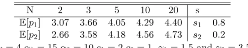
Table 1: Expected prices and the number of firms
N 2 3 5 10 20 s
E[p1] 3.07 3.66 4.05 4.29 4.40 s1 0.8
E[p2] 2.66 3.58 4.18 4.56 4.73 s2 0.2
cf = 4,α1 = 15,α2 = 10,c1 = 2,c2 = 1,γ1= 1.5 and γ2 = 3.5
of this section. Moreover, when the number of competitiors increase, the probability of
winning the attention of the representative consumer reduces, given that all of the firms
have the same probabilityex-ante to be victorious. Therefore, we must have an increase in
the expected prices to maintainex-ante profits equal to zero. In Table1, we give a numerical
example20 in which we vary the number of market participants while maintaining constant
all other parameters. As noted, expected prices are higher as the number of firms increase.
Consumers just buy from the store with the best combination of prices and in-store space
allocation. As shelf space will be constant in the entire distribution of prices, this translates
into consumers buying from the lowest prices store or, as refered, from the store with the
lowest profit. In this sense, what really matters in terms of consumer’s welfare is the expected
value of the lowest price, which greatly differ from those given in table1.
The distribution function of the minimum β, in other words, the distribution function of
the profit attained by the firm which wins the price war,Fmin:R→[0,1], is defined as:21
Fmin(β) =
0 β <0
1− Cf β+Cf
1
N−1
−
Cf
α1+α2 N1
−1
1−
Cf
α1+α2 N1 −1 N
β ∈[0, α1+α2−Cf]
1 β > α1+α2−Cf
(27)
In Table 2 we present the expected values of the lowest prices set by firms. As seen in
the table, they are decreasing in the number of firms. Since consumers just buy from the
20We acknowledge that this example was computed based just on necessary first order conditions and
subject to the same problems regarding sufficiency stated previously.
21In order to find this function, one must remember that:
Fmin(β) =P rob[βj> β ∀j∈ {1, ..., N}],
= 1−(1−F(β))N.
lowest price store, the price paid by them is decreasing inN. This result might not be quite
intuitive if one accounts for the fact that firms must pay a fixed cost to post prices in the
market. Nevertheless, as N increases, the probability of entry, given previously byα falls.
Therefore, an increase in the number of possible entrants in the market benefits ex-ante
the consumer if she is risk neutral. Since firms allways work with ex-ante zero profits, an
increase inN increases welfare in the economy with risk neutral participants.
Table 2: Expected values of the lowest prices and the number of firms
N 2 3 5 10 20
E[pmin1 ] 2.21 2.19 2.16 2.13 2.12
E[pmin2 ] 1.33 1.29 1.24 1.20 1.18
cf = 4,α1 = 15,α2 = 10,c1 = 2,c2 = 1,γ1= 1.5 and γ2 = 3.5
4
Conclusion
There are few works in economics concerned with the problem of shelf space allocation.
We present two possible reasons for this. First, data about shelf space allocation may be
scarce and difficult to obtain.22 Second, there is still no consensus on a good theory to
explain price dispersion and therefore about retail competition, which is mainly price driven.
In this sense, this work is an attempt to shed some light on the problem of in-store display
of products from a purely economics persperctive.
We have presented a new way to look at this problem. The in-store allocation of products
is modeled directly in consumers’ utility function which impose the importance of shelf space
allocation to retailers. Fixed costs prevent existence of pure strategy equilibria in the retail
competition game just as in Baye and Morgan (2001) and Sharkey and Sibley (1993),
therefore some kind of dispersion must follow. Unfortunately, it can’t be said anything
further by just looking at the general model as it is highly dependent on the functional form
of the utility function. We have chosen then to present a simple version of the model for a
special case of the utility function.
In this special case, an interesting result emerge. Although retailers are able to choose
22Even these data is obtained it may not be a simple object. For instance, the display of products in-store
any vector of shelf space allocation in the simplex, it is shown that shelf space allocation
does not to vary in the cross-section of stores. It is not optimally in equilibrium to carry over
the retail competition to the decision on shelf allocation. Retail competion resumes itself to
competion on prices, which are therefore dispersed in the equilibrium. As argued, we have
managed to reconcile with this model two distinct stylized facts about retail competion: that
prices are dispersed in equilibrium and that shelf space allocation changes unfrequently.
References
Albeniz, V. and G. Roels, “Competing for Shelf Space,” SSRN eLibrary, 2007.
Baye, M.R. and J. Morgan, “Information gatekeepers on the internet and the
compet-itiveness of homogeneous product markets,” American Economic Review, 2001, pp. 454–
474.
and , “Price Dispersion in the Lab and on the Internet: Theory and Evidence,”RAND
Journal of Economics, 2004, pp. 449–466.
Bliss, C., “A theory of retail pricing,” The Journal of Industrial Economics, 1988, 36 (4),
375–391.
Boiteux, M., “Sur la gestion des monopoles publics astreints `a l’´equilibre budg´etaire,”
Econometrica, Journal of the Econometric Society, 1956, 24(1), 22–40.
Braido, L.H.B., “Multiproduct price competition with heterogeneous consumers and
non-convex costs,” Journal of Mathematical Economics, 2009, 45, 526–534.
Bultez, A. and P. Naert, “SH.ARP: Shelf allocation for retailers’ profit,” Marketing
Science, 1988, pp. 211–231.
Corstjens, M. and P. Doyle, “A model for optimizing retail space allocations,”
Manage-ment Science, 1981, 27(7), 822–833.
Curhan, R.C., “The relationship between shelf space and unit sales in supermarkets,”
Dreze, X., S.J. Hoch, and M.E. Purk, “Shelf management and space elasticity,”Journal
of Retailing, 1994,70, 301–301.
Kreps, D.M. and J.A. Scheinkman, “Quantity precommitment and Bertrand
competi-tion yield Cournot outcomes,” The Bell Journal of Economics, 1983, pp. 326–337.
Kruse, J.B., S. Rassenti, S.S. Reynolds, and V.L. Smith, “Bertrand-Edgeworth
competition in experimental markets,”Econometrica: Journal of the Econometric Society,
1994, pp. 343–371.
Marquez, R., “A note on Bertrand competition with asymmetric fixed costs,” Economics
Letters, 1997, pp. 87–96.
Morgan, J., H. Orzen, and M. Sefton, “A laboratory study of advertising and price
competition,”European Economic Review, 2006, 50(2), 323–347.
Pratt, J.W., D.A. Wise, and R. Zeckhauser, “Price differences in almost competitive
markets,” The Quarterly Journal of Economics, 1979,93(2), 189–211.
Sharkey, W.W. and D.S. Sibley, “A Bertrand model of pricing and entry,” Economics
Letters, 1993, 41(2), 199–206.
Simon, L.K. and W.R. Zame, “Discontinuous games and endogenous sharing rules,”
Econometrica: Journal of the Econometric Society, 1990, pp. 861–872.
Stahl, D.O., “Oligopolistic pricing with sequential consumer search,” The American
Eco-nomic Review, 1989, pp. 700–712.
van Dijk, A., H.J. van Heerde, P.S.H. Leeflang, and D.R. Wittink,
“Similarity-based spatial methods to estimate shelf space elasticities,” Quantitative Marketing and
Economics, 2004, 2 (3), 257–277.
Varian, H.R., “A model of sales,”The American Economic Review, 1980, pp. 651–659.
Winter, R.A., “Vertical control and price versus nonprice competition,” The Quarterly
Appendices
A
Optimal shelf allocation and pricing
From the first order condition and using the fact that ∂xj
∂sj =−γj
∂xj
∂pj:
−xj+µ[(pj −cj)
∂xj
∂pj
] =−φ
γj
, j= 1,2. (28)
Subtracting equation (28) from (15):
µxj =
φ γj
j= 1,2⇒ x1
x2 = γ2
γ1
. (29)
Substituting equation (29) in the first restriction of the optimization problem given by
(14) one ends up with:
x2[
γ2
γ1
(p1−c1) + (p2−c2)] =β+Cf, (30)
1
γ1 α2
p2−γ2s2[γ2(p1−c1) +γ1(p2−c2)] =β+Cf. (31)
From equation (15):
xj(µ−1) +µ(pj−cj)
∂xj
∂pj
=0, (32)
xj (pj−cj)∂x∂pjj
= µ
1−µ, (33)
pj−γjsj
pj −cj
= µ
µ−1, j= 1,2. (34)
From equations (29) and (34):
γ1α1 γ2α2
= p1−γ1s1
p2−γ2s2
= p1−c1
p2−c2
Substituting equation (35) in (31):
1
γ1
α2
p2−γ2s2 [γ2
γ1α1
γ2α2
(p2−c2) +γ1(p2−c2)] =β+Cf, (36)
(α1+α2)(p2−c2)
p2−γ2s2
=β+Cf, (37)
(α1+α2)(p2−c2) =(β+Cf)(p2−γ2s2), (38)
[α1+α2−(β+Cf)]p2 =(α1+α2)c2−γ2(β+Cf)s2, (39)
p2=
α1+α2
α1+α2−(β+Cf)
c2−
γ2(β+Cf)
α1+α2−(β+Cf)
s2. (40)
In a similar manner:
p1 =
α1+α2
α1+α2−(β+Cf)
c1−
γ1(β+Cf)
α1+α2−(β+Cf)
s1. (41)
From equations (40), (41) and the second restriction in (14):
(p1−c1) =
β+Cf
α1+α2−(β+Cf)
c1−
γ1(β+Cf)
α1+α2−(β+Cf)
(1−s2), (42)
(p2−c2) =
β+Cf
α1+α2−(β+Cf)
c2−
γ2(β+Cf)
α1+α2−(β+Cf)
s2. (43)
Substituting equations (42) and (43) in (31):
1
γ1
α2
p2−γ2s2
(β+Cf)(γ2c1+γ1c2−γ1γ2)
α1+α2−(β+Cf)
=β+Cf, (44)
α2
γ1
γ2c1+γ1c2−γ1γ2
α1+α2−(β+Cf)
=p2−γ2s2. (45)
From equation (40):
p2−γ2s2 =
α1+α2
α1+α2−(β+Cf)
c2−
γ2(α1+α2)
α1+α2−(β+Cf)
s2. (46)
α2
γ1
(γ2c1+γ1c2−γ1γ2) =(α1+α2)(c2−γ2s2), (47)
s2=
c2
γ2 − α2
γ1γ2
γ2c1+γ1c2−γ1γ2
α1+α2 . (48)
Similarly,
s1= c1
γ1
− α1
γ1γ2
γ2c1+γ1c2−γ1γ2 α1+α2
. (49)
Finnaly, one may obtain prices by substituting (48) and (49) in (40) and (41), respectively:
p1=c1+ α1
α1+α2
β+Cf
α1+α2−(β+Cf)
γ1c2+γ2c1−γ1γ2 γ2
, (50)
p2=c2+
α2
α1+α2
β+Cf
α1+α2−(β+Cf)
γ1c2+γ2c1−γ1γ2
γ1
. (51)
B
Proof of Proposition
1
In the case ofngoods, the steps followed to compute the equilibrium shelf space allocation
and prices are very similar to those taken when stores sell just two goods. Firms problem is
basically the same as the one given by equation (14).
Note that the first steps taken in Appendix A don’t require the two goods assumption
and are true in thengoods case.
We are then left with a new set of equations:
xi
xj =γj
γi
, ∀i, j= 1,· · · , n; (52)
γiαi
γjαj
=pi−γisi
pj −γjsj
= pi−ci
pj−cj
, ∀i, j = 1,· · · , n. (53)
Substituting again the previous equations in the first restriction of the maximization
γi
αi
pi−γisi
X
j
pj−cj
γj
=β+Cf, ∀i= 1,· · · , n. (54)
From equation (53), we have that:
∀j,(pj−cj) = (pi−ci)
γjαj
γiαi
∀i; (55)
which can replace the appropriate terms in equation (54). Doing this gives us:
pi−ci
pi−γisi
X
j
αj =β+Cf, (56)
(pi−ci)
X
j
αj =(pi−γisi)(β+Cf), (57)
pi =
P
jαj
P
jαj −(β+Cf)
ci−
γi(β+Cf)
P
jαj−(β+Cf)
si, (58)
pi−ci =
β+Cf
P
jαj −(β+Cf)
ci−
γi(β+Cf)
P
jαj−(β+Cf)
si, (59)
pi−ci =
β+Cf
P
jαj −(β+Cf)
[ci−γisi]; ∀i= 1,· · ·, n. (60)
We may replace (59) in equation (54) and obtain:
γi
αi
pi−γisi
β+Cf
P
jαj−(β+Cf) [X
j
(cj−γjsj)], ∀i= 1,· · · , n. (61)
But pi−γisi can be writen as:
pi−γisi =
(ci−γisi)Pjαj
P
jαj−(β+Cf)
(62)
Substituting in equation (61), we come up with the following system of equations:
γiαi (ci−γisi)Pjαj
X
j
(cj−γjsj)
=1, ∀i= 1,· · ·, n; (63)
X
j
Regard that the system above determines the full vector of shelf space allocation s and
that the system does not depend onβ, the firms’ profit level, which is, in the end, the random
component of firms strategy.
C
Consumers’ expenditure in the firms’ products
Using equations (21), (22) and (18):
X
j=1,2
xj(β)pj(β) =
c1+
α1
α1+α2
(β+Cf)(γ2c1+γ1c2−γ1γ2)
γ2(α1+α2−(β+Cf))
γ2(α1+α2−(β+Cf))
γ2c1+γ1c2−γ1γ2)
+
c1+
α2
α1+α2
(β+Cf)(γ2c1+γ1c2−γ1γ2)
γ1(α1+α2−(β+Cf))
γ1(α1+α2−(β+Cf))
γ2c1+γ1c2−γ1γ2)
.
(65)
Which greatly simplifies to
X
j=1,2
xj(β)pj(β) =
(c1γ2+c2γ1)(α1+α2−(β+cf))
c1γ2+c2γ1−γ1γ2
+ (β+cf), (66)
= (γ2c1+γ1c2)(α1+α2)−γ1γ2(β+Cf))
γ2c1+γ1c2−γ1γ2