Consumption-wealth ratio and expected stock returns: evidence from panel data

FUNDAÇÃO GETÚLIO VARGAS

ESCOLA DE PÓS-GRADUAÇÃO EM

ECONOMIA

Andressa Souza Campos Monteiro de Castro

Consumption-Wealth Ratio and Expected Stock Returns:

Evidence from Panel Data

Andressa Souza Campos Monteiro de Castro

Consumption-Wealth Ratio and Expected Stock Returns:

Evidence from Panel Data

Dissertação submetida a Escola de Pós-Graduação em Economia como requisito parcial para a obtenção do grau de Mestre em Economia.

Área de Concentração: Macroeconometria

Orientador: João Victor Issler

Ficha catalográfica elaborada pela Biblioteca Mario Henrique Simonsen/FGV

Castro, Andressa Souza Campos Monteiro de

Consumption-wealth ratio and expected stock returns: evidence from panel data / Andressa Souza Campos Monteiro de Castro. – 2015.

27 f.

Dissertação (mestrado) - Fundação Getulio Vargas, Escola de Pós-Graduação em Economia.

Orientador: João Victor Issler. Inclui bibliografia.

1. Consumo (Economia). 2. Macroeconomia. 3. Mercado financeiro. 4. Ações (Finanças). 5. Cointegração. I. Issler, João Victor. II. Fundação Getulio Vargas. Escola de Pós-Graduação em Economia. III. Título.

Abstract

This paper investigates the role of consumption-wealth ratio on predicting future stock returns through a panel approach. We follow the theoretical framework proposed by Lettau and Ludvigson (2001), in which a model derived from a nonlinear consumer’s budget constraint is used to settle the link between consumption-wealth ratio and stock returns. Using G7’s quarterly aggregate and financial data ranging from the first quarter of 1981 to the first quarter of 2014, we set an unbalanced panel that we use for both estimating the parameters of the cointegrating residual from the shared trend among consumption, asset wealth and labor income,cay, and performing in and

out-of-sample forecasting regressions. Due to the panel structure, we propose differ-ent methodologies of estimating cay and making forecasts from the one applied by

Lettau and Ludvigson (2001). The results indicate thatcaydis in fact a strong and

ro-bust predictor of future stock return at intermediate and long horizons, but presents a poor performance on predicting one or two-quarter-ahead stock returns.

Contents

1 Introduction 7

2 Theoretical Framework 9

3 Aggregate and Financial Data 11

4 Estimatingcay 13

5 Forecasting Stock Returns 15

6 Robustness Checks 21

7 Out-of-Sample Tests 23

8 Conclusion 26

List of Figures

1 Excess Returns and Estimatedcay . . . 16

List of Tables

2 Johansen Fisher Panel Cointegrating Test . . . 14

3 Panel Cointegrating Vector Estimates . . . 15

4 Forecasting Stock Returns . . . 18

5 Long-Horizon Regressions . . . 19

6 Robustness Regressions . . . 22

7 Out-of-Sample Nested Comparisons . . . 24

1 Introduction

The link between macroeconomics and financial markets has long driven a great amount of empirical work in macroeconometric literature. Motivated by the well known pre-dictability of stock returns (Campbell and Shiller, 1988; Fama and French, 1988; Pesaran and Timmermann, 1995), a branch of this literature has concerned about the forecasting power of macroeconomic variables over future excess returns. There is still little empirical evidence that support such theories, though.

In a seminal paper, Lettau and Ludvigson (2001) study the role of transitory devia-tions from the common trend in consumption, asset holdings and labor income for pre-dicting stock market fluctuations. They show that, according to forward-looking models of consumer behavior, when investors expect higher future returns, they react by rising current consumption out of its shared trend with asset wealth and labor income in or-der to maintain a flat consumption path, avoiding sharp variations. Therefore, instead of expecting a subsequent raise on aggregate consumption in a financial market boom sce-nario, when returns are high, there is an anticipation of this consumption growth. That way, the consumption-wealth ratio may carry information about the future dynamics of excess returns.

Despite the strong empirical evidence provided by Lettau and Ludvigson (2001) en-suring the forecasting power of consumption-wealth ratio over excess stock returns on U.S. market, there was practically no evolution about this issue in further work. Ioan-nidis et al. (2006), Tsuji (2009) and Gao and Huang (2008) extended the analysis to other countries, following the methodology proposed by Lettau and Ludvigson (2001) to esti-mate the consumption-wealth ratio and explain either future stock returns or the cross-section of stock returns. Nitschka (2010) have also applied the same estimation method, but used the consumption-wealth ratio of U.S. as a predictor of foreign stock returns, from an American’s investor point of view. Most importantly, in all works that include more than one country, the analysis was done separately for each country through time series estimations.

panel-based tests, such as unit root and contegration tests, have higher power than tests based on individual time series. With this in mind, using G7’s quarterly aggregate and fi-nancial data, we verify if consumption-wealth ratio is indeed a strong predictor of future excess stock returns.

After checking the cointegrating relationship among consumption, asset wealth and labor income with a panel version of Johansen (1991) test, we estimate the error correc-tion term of a single vector error correccorrec-tion (VEC) for the entire panel, with consumpcorrec-tion, asset wealth and labor income as endogenous variables. The estimated error correction term is what we calldcay, which represents the estimated consumption-wealth ratio.

Alter-natively, we also compute seven different VEC’s for each country, obtaining one specific cointegrating vector for each one of them, which we use to build adcay_h with heteroge-neous parameters and compare its performance on forecasting returns with the perfor-mance of thecayestimated from the single cointegrating vector.

Next, we make several forecasting regressions to investigate the power of _dcay and

d

cayhas predictors for short and long-term excess stock returns. We find thatdcayhhave no

power on predicting returns, in contrast to dcay, which forecasting power increases over

the time horizon. We also include in these regressions some financial variables widely used to predict stock returns. The results indicate thatdcay is the sole robust and strong

predictor of future excess returns, but only for two years onward. Non of the predictive variables has shown any capacity of predicting one-quarter-ahead returns.

The remainder of this work proceeds as follows. The next section presents a brief re-view of the theoretical framework which establishes the relationship between consumption-wealth ratio and expected stock returns. In Section 2, we thoroughly detail the aggregate and financial data that we use to construct our panel. Section 3 shows the VEC estimates from the cointegrating relation among consumption, asset wealth and labor income and specifies how we build the estimatedcay. Section 4 reports the results of forecasting

re-gressions over several time horizons to investigate the predictive power ofcayand some

financial variables widely used to forecast stock returns. In Section 5, we re-estimate the forecasting regressions using a different method to check the robustness of the previous results. Finally, on Section 6, we perform out-of-sample forecasts and compare the MSE of models that include_dcaywith the ones that do not, in order to see if this variable carries

2 Theoretical Framework

To settle the link between consumption-wealth ratio and expected stock returns, consider a representative consumer who invests his total wealth, receiving a time-varying return. Let Wt and Ct be the aggregate wealth and aggregate consumption in period t,

respec-tively. Rw,t+1 is the net return on aggregate invested wealth. The intertemporal budget

constraint faced by this agent is:

Wt+1 = (1 +Rw,t+1)(Wt−Ct). (1)

To deal with this expression, Campbell and Mankiw (1989) suggest log-linearizing it, obtaining

∆wt+1 ≈rw,t+1+ (1−1/ρw)(ct−wt) +k1, (2)

where the lower case letters are used to denote the logs of the corresponding variables,

rw,t+1 ≡ log(1 +R), ρw is the steady-state proportion of investment on wealth andk1 is a

constant.

If the consumption-wealth ratio is stationary, it is possible to solve this equation for-ward. Thus, taking the conditional expectation and assuming that the transversality con-dition

limi→∞Et[ρ

i

w(ct+i−wt+i)] = 0holds, the log consumption-wealth may be written as

ct−wt=Et

∞

X

i=1 ρi

w(rw,t+i−∆ct+i) +k2 (3)

which means that the return to wealth or the consumption growth or both could be pre-dicted by consumption-wealth ratio.

Defining aggregate wealth as asset wealth plus human capital Wt = At+Ht, the log

aggregate wealth may be approximated as

wt ≈γat+ (1−γ)ht+k3, (4)

where γ is the average share of asset holdings in total wealth. Furthermore, Campbell (1996) shows that the return to aggregate wealth, which is given by

may be log-linearized to get to a tractable intertemporal model with constant coefficients:

rw,t≈γra,t+ (1−γ)rh,t +k4. (6)

Substituting(4)and(6)into (3), gives

ct−γat−(1−γ)ht=Et

∞

X

i=1 ρi

w[γra,t+i+ (1−γ)rh,t+i−∆ct+i] +k5. (7)

Unfortunately, as noted by Campbell, human capital is not directly observable. What we do observe is labor income, which can be interpreted as the dividend on human wealth, implying that

(1 +Rh,t+1) =

(Ht+1+Yt+1) Ht

. (8)

Once more, log-linearizing this expression, we obtain

rh,t+1 ≈ρhht+1+ (1−ρh)yt+1−ht+k6, (9)

where ρh is the steady-state proportion H/(H +Y). Solving it forward, taking the

ex-pectation and imposing thatlimi→∞E_t[ρ

i

h(ht+i−yt+i)] = 0, the log human capital can be

described as

ht =yt+Et

∞

X

i=1 ρi

h(∆yt+i−rh,t+i) +k7. (10)

Lettau and Ludvigson (2001) show that the nonstationary component of human capi-tal is captured by labor income, implying thatht=κ+yt+µt, whereκis a constant. It is

easy to see from(10)thatµt =Et

P∞

i=1ρ

i

h(∆yt+i−rh,t+i). This term is a stationary random

variable, since we are assuming that∆ytis stationary - labor income has a unit root - and

that the return on human wealth is practically constant.

Replacing the log of human wealth in expression(7) by the one obtained in(10), it is possible to rewrite the log consumption-wealth ratio in terms of observable variables:

cayt = ct−γat−(1−γ)yt (11)

= Et

∞

X

i=1 ρi

w[γra,t+i+ (1−γ)rh,t+i−∆ct+i] + (1−γ)µt+k8. (12)

Under the assumption thatrw,t,∆ctand∆ytare stationary1, equations(11)and(12)imply

1_{We test the evidence of unit root process in consumption and labor income in our panel data. Both don’t}

thatct,atandytare cointegrated andct−γat−(1−γ)ytis the cointegrating residual labelled

ascayt, where(1,−γ,−(1−γ))is the cointegrating vector (Lettau and Ludvigson, 2004).

Besides, according to(11) and (12) we may say that cayt Granger-causes the right-hand

term in brackets. Therefore, provided that the expected future returns on human capital and consumption growth are not too variable, movements oncaytshould forecast changes

in asset returns2_,PH

i=1ra,t+i,H = 1,2, ...∞.

This result is by and large consistent with a wide range of forward-looking models of investor behavior, where the agents, disliking sharp fluctuations on consumption, will attempt to smooth out transitory movements in asset wealth due to variations in expected asset returns. For instance, when higher returns are expected in the future, the forward-looking investors will currently increase their consumption out of their asset wealth and labor income, rising consumption above its common trend with those variables. Sum-ming up, the detachment of consumption from its shared trend with asset wealth and labor income is likely to be a predictor of stock returns. Our work here is to estimatecay

using consumption, labor income and asset holdings data, and through a panel approach to verify whether this estimatedcayis a strong predictor of real returns and excess returns

on stock indexes.

3 Aggregate and Financial Data

We work with a typical panel of macroeconomic data, which has a small individual di-mension and a large time didi-mension. More specifically, we analyze an unbalanced panel for G7’s countries3_{: Canada, France, Germany, Italy, Japan, United Kingdom and United}

States. All aggregate variables are quarterly, seasonally adjusted, per capita, measured in 2010 country’s own currency. To deflate data we use the CPI from International Financial Statistics (IFS), the FMI’s database, and for quarterly population we make an interpola-tion on annual data provided by OCDE.

The consumption data is private final consumption expenditure from National Ac-counts Statistics of OCDE’s database. Labor income is represented by compensation of employees and provided by Federal Reserve Economic Data (FRED) of the Federal Re-serve Bank of St. Louis, but the original source is OCDE as well. Asset holdings data was taken separately from each country’s central banks. As mentioned, the panel is

un-linear trends.

2_{Lettau and Ludvigson (2001) find thatcay}

tis a strong predictor of excess returns on aggregate US stock

market indexes for both short and long run.

3_{The reason for choosing G7 is the lack of data availability for other countries in quarterly frequency,}

balanced, thus the length of period is different for each country. More specifically, the length of period for all aggregate data is given by the length of period observed for asset holdings, once there are less observations for this variable than for consumption and in-come. Therefore, Table 1 specifies the sources, the kind of data used as asset wealth and the length of period for each country.

Table 1: Data Sources

Canada CANSIM, Statistics Canada: Net worth of households and (1990Q1 - 2014Q1) non-profit institutions serving households (NPISH)

France Webstat, Banque de France: Net financial assets

(1996Q1 - 2014Q1) of households and NPISH

Germany Deutsche Bundesbank: Financial Asset

(1991Q1 - 2014Q1) of households and NPISH

Italy BDS, Banca D’Italia: Total financial instruments

(1995Q1 - 2014Q1) held by households and NPISH

Japan _{Bank of Japan: Total assets of households}

(1997Q4 - 2014Q1)

United Kingdom Bank of England: Financial assets

(1997Q1 - 2014Q1) of households and NPISH

United States Board of Governors of the Federal Reserve System:

(1981Q1 - 2014Q1) Net worth of households and NPISH

The main financial data are real returns and excess returns on stock indexes. In order to obtain the log of real returnsrt, we take for each country the quarterly closing prices,

adjusted for dividends, of the stock indexes provided by Bloomberg, deflate them using the seasonally adjusted CPI from IFS, divide period t by period t − 1 values and take the log. The stock indexes used are S&P/TSX composite index for Canada, CAC 40 for France, DAX for Germany, FTSEMIB for Italy, Nikkei 225 for Japan, FTSE 100 for United Kingdom and S&P 500 for United States. To obtain quarterly log of excess returns rt−

rf,t, we need to specify the risk-free rate rf,t. The raw data is the percent per annum

treasury bill rate from government securities for each country, taken from IFS. To get to the quarterly log of real return on the T-bill, we sum a unit to the percent rate, convert the annual returns into quarterly returns, deflate them using a seasonally adjusted inflation rate from the CPI and take the log.

power betweencayand these variables. Letd−pdenote the dividend yield, wheredis the log of quarterly dividends per share and pis the log of the stock index. Since Campbell and Shiller (1988), this variable has been widely used to forecast excess returns4_{, specially}

for long horizons. Following Lamont (1998), the payout ratio is represented by d −e,

wheree is the log of quarterly earnings per share. As well as the stock index, both

divi-dends per share and earnings per share are provided by Bloomberg. Finally, we build the relative bill rate RREL subtracting from the T-bill rate its 12-month backward moving

average, a method suggested by Hodrick (1992). For now on, when we refer to any of this variables, aggregate or financial, we are already considering them in logs.

4 Estimating

cay

Before estimatingcay, the cointegrating residual of the shared trend in consumption,

la-bor income and asset wealth, we test whether each variable passes a unit root test, since we are assuming a cointegrating process between these variables. Therefore, we perform a panel unit root test proposed by Maddala and Wu (1999), which consists in a Fisher (1932) test5 _{that combine the significance levels from individual unit root tests, such as}

Phillips-Perron (PP) and Augmented Dickey-Fuller (ADF), to derive a panel-specific re-sult. Thus we test for unit root in level for each variable, including in the test equation individual intercepts and individual trends for each country. For all three variables in both tests, PP and ADF, the null hypothesis of presence of unit root is not rejected at a ten percent significance level6_{, which is a good evidence of each process being integrated.}

Hence, we conduct another Fisher-type test also suggested by Maddala and Wu (1999) using a Johansen (1991) procedure to determine the number of cointegrating relations among those three variables in the panel. The results summarized on Table 2 strongly indicate that there is indeed a single cointegrating vector for consumption, asset wealth and labor income.

Once the presence of a cointegrating vector is supported by these results, the next step is to estimate the parameters of this vector, which we do in two separate ways. On the first estimation, we make a single Vector Error Correction (VEC) for the entire panel, assuming homogeneity in the cointegrating parameters. On the second one, we make

4_{Campbell and Shiller (1988) show that the log dividend-price ratio may be written as d}

t −pt = EtP

∞

j=1ρ j

a(ra,t+j−∆dt+j), which means that if the dividend-price ratio is high, agents must be

expect-ing either high future asset returns or low dividend growth rates.

5_{We choose the Fisher test due to the structure of our data. The asymptotic validity for this test depend}

Table 2: Johansen Fisher Panel Cointegrating Test Hypothesized Fisher Stat.

P-value* Fisher Stat. P-value*

Num. of Coint. Trace Test Max-Eigen Test

None 40.28 0.0002 36.84 0.0008

At most 1 16.56 0.2805 10.77 0.7044

At most 2 28.45 0.0124 28.45 0.0124

This table reports the panel cointegration test on consumption, asset wealth and income pooled series, assuming that there is a linear deterministic trend in data, including an intercept in the cointegration equation, and using one lag in difference (two lags in level) on the VAR tested.

*Probabilities are computed using asymptoticχ2_{distribution.}

seven VEC’s, one for each country, taking into account the presence of heterogeneity in the cointegrating parameters. On both procedures, we include consumption, asset wealth and labor income as endogenous variables and make the same assumptions we have made for the panel cointegration test - linear deterministic trend in data, an intercept in the cointegration equation and one lag in difference for the endogenous variables -, imposing one cointegrating relationship among the three variables.

On the first VEC estimation, we assume that the cointegration structure is given by

ci,t =βaai,t+βyyi,tdisregarding the constant included in the cointegrating equation, where

βa and βy are the cointegrating parameters to be estimated, andci,t, ai,t and yi,t are

con-sumption, asset wealth and labor income for each country in each period, respectively. Note here that the homogeneity is captured by the invariant parameters βa and βy. We

report in Table 3 the estimates of this parameters for the panel, obtained on the first part of the VEC7_{estimation and omit the rest of the VEC output.}

With the parameters estimates we can easily construct the variable dcay, which is the

error correction term in one lag forward (current time) and, ignoring the constant, is given bydcay_i,t =ci,t−βbaai,t−βbyyi,t. Lettau and Ludvigson (2004) argument that this

cointegra-tion residual must be covariance stacointegra-tionary, instead of stacointegra-tionary around a deterministic trend. If the contrary was true, it would imply that either consumption or aggregate

7_{With one lag in difference, linear trend and one cointegrating relationship, we estimate the following}

VEC through a pooled OLS.

∆ci,t=α1(ci,t−1−βaai,t−1−βyyi,t−1−µ) +γ11∆ci,t−1+γ12∆ai,t−1+γ13∆yi,t−1+η1+ǫ1,i,t

∆ai,t=α2(ci,t−1−βaai,t−1−βyyi,t−1−µ) +γ21∆ci,t−1+γ22∆ai,t−1+γ23∆yi,t−1+η2+ǫ2,i,t

∆yi,t=α3(ci,t−1−βaai,t−1−βyyi,t−1−µ) +γ31∆ci,t−1+γ32∆ai,t−1+γ33∆yi,t−1+η3+ǫ3,i,t

The right-hand side variable in parenthesis is the error correction term. In long run equilibrium, this term should be zero. However, if any variable of this term deviates from the long run equilibrium, the error correction term would be nonzero and the other variables would adjust to restore the equilibrium relation. The coefficientsαmeasure the speed of adjustment of each endogenous variable towards the equilibrium

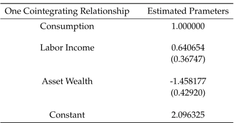
Table 3: Panel Cointegrating Vector Estimates One Cointegrating Relationship Estimated Prameters

Consumption 1.000000

Labor Income 0.640654

(0.36747)

Asset Wealth -1.458177

(0.42920)

Constant 2.096325

This table presents the estimated parameters of the cointegrating vector(1,−_βb_y,−_βba),

with respective standard errors in parenthesis. On the specification, we assume there is a linear deterministic trend in data, including an intercept in the cointegrating equation, use one lag in difference and impose one cointegrating relationship. 594 observations are included in this estimation after adjustments. Both estimates are statistically significant at a two-sided 10% level, computed using asymptotic Normal distribution.

wealth would eventually become an infinitesimal fraction of the other, violating the bud-get set used as starting point. Therefore, as a closure for this estimation, we check ifdcayis

stationary by performing the Fisher-ADF and PP panel unit root tests, including individ-ual intercepts but not any trends. We obtain p-values of 2.67% and 6.05% for ADF and PP Fisher tests respectively, confirming thatdcay is indeed stationary.

Then we proceed to the second VEC estimation, which has an heterogeneous coin-tegration structure, i.e. ci,t = βa,iai,t + βy,iyi,t, ignoring the cointegration constant once

more. Thus, to estimate the cointagrating parameters, we perform separated VEC’s for each country (not reported here). The estimated heterogeneous cay is then given by

d

cayhi,t =ci,t−βba,iai,t−βby,iyi,t. Then, we make the same panel unit root tests we have made

fordcay to check the stationarity ofcaydh. The presence of unit root is strongly rejected on

both tests, such that even with different cointegrating parameters for each country, the variablecaydhcan be considered stationary on the panel as a whole.

5 Forecasting Stock Returns

In this section, we focus on verifying the power of cay as a predictive variable for real

returns and excess returns in a panel structure. The intuition here is that variations on

cay should precede variations on stock returns, since theoretically, the forward-looking

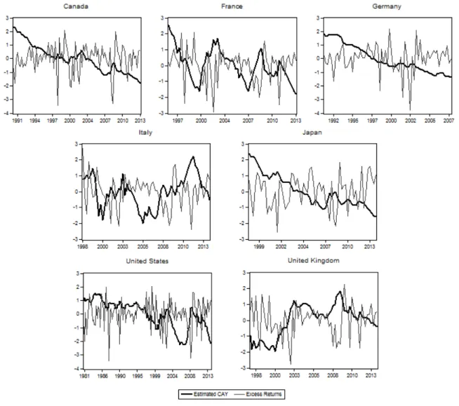
Although we restrict our analysis to a panel approach, it is interesting to illustrate the relationship between cay and stock returns and to see how these variables evolve through time, which has do be done separately for each country. For this purpose, we make individual graphs with both log excess returns - returns on stock indexes minus the return on T-bill - and_dcay normalized series, displayed in Figure 1.

Figure 1: Excess Returns and Estimatedcay

This figure shows, for some countries such as France, Italy, United Kingdom and USA, sharp variations of_dcaypreceding spikes in excess returns, for both positive and negative

fluctuations, specially after year 2000. It is also interesting to notice that recently most countries have presented a pronounced decreasing indcay. Thus, if this variable is indeed

Another feature of dcay, which can be noticed in some graphs of Figure 1, is that by and large this variable is counter-cyclical. In fact, when we make a panel regression of consumption growth on contemporaneous _dcay controlling for cross section fixed effects,

we obtain a coefficient of−0.005181statistically significant at1%level. This is consistent with a framework studied by Campbell and Cochrane (1999), in which booms, character-ized by high income growth, are periods when consumption rises above habit, inducing a decline in risk aversion. This decline in risk aversion in turn leads to greater demand for risky assets, which reinforces its increase caused by the high income growth. Thus, despite the increase in consumption pushing dcay upwards, the growth on asset wealth

overcomes this effect, causing a decline on consumption wealth ratio. For instance, in all countries in Figure 1 there was a remarkable increase ofdcayfrom 2007 to 2008, when the financial crisis was at its peak.

We now turn our attention back to the forecasting power of cay over the panel stock

returns data. First, we make some one-quarter-ahead regressions with real returns and excess returns as dependent variables and both_dcayandcay_dhplus other financial variables

as regressors, including cross-section fixed effects. In all of these regressions, we make White cross-section corrections8 _{to the standard errors, obtaining estimators robust to}

cross-section heteroskedasticity and cross-section correlation. The estimation results are reported on Table 4.

Regressions with one-period lag of the dependent variable as a regressor are also com-puted on Table 4. It is well known that the LSDV (least squares dummy variable) - the fixed effects model we have used in the previous regressions - with a lagged dependent variable generates biased estimates when the time dimension of the panel is small (Judson and Owen, 1999). Nevertheless, Nickell (1981) derives an expression for the bias showing that it goes to zero when T approaches infinity. Thus for our purposes LSDV continues

performing well, considering that the number of periods in our data is sufficiently large9_.

We use the White cross-section correction in these regressions as well.

The results in Table 4 show that, at this time horizon length - just one quarter ahead - both dcay and caydh are not able to predict stock returns, since they are not statistically

8_{This method considers the pool regression as multivariate regressions with one equation for each}

cross-section, and computes for the system of equations robust standard errors. The robust variance matrix estimator is given byAvar( ˆβ) ≡

N T N T −K

(PtX

′

tXt)

−1

(PtX

′

tˆǫtǫˆ′tXt) (PtX

′

tXt)

−1

, whereN T is the

total number of stacked observations and K is the total number of estimated parameters. See Arellano

(1987) and Wooldridge (2010). We choose this estimator because of its consistency for panels with largeT

and fixedN.

9_{We work with an unbalanced panel in which the time dimension goes from 66 to 134 observations.}

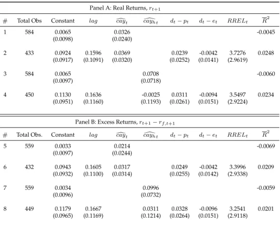
Table 4: Forecasting Stock Returns

Panel A: Real Returns,rt+1

# Total Obs Constant lag dcayt cay[ht dt−_{pt dt}−_{et RRELt R}2

1 584 0.0065 0.0326 -0.0045 (0.0098) (0.0240)

2 433 0.0924 0.1596 0.0369 0.0239 -0.0042 3.7276 0.0248 (0.0917) (0.1091) (0.0320) (0.0252) (0.0141) (2.9619)

3 584 0.0065 0.0708 -0.0060 (0.0097) (0.0718)

4 450 0.1130 0.1636 -0.0025 0.0311 -0.0094 3.5497 0.0234 (0.0951) (0.1160) (0.1193) (0.0261) (0.0151) (2.9224)

Panel B: Excess Returns,rt+1−_rf,t+1

# Total Obs. Constant lag dcayt cay[ht dt−_{pt dt}−_{et RRELt R}2

5 559 0.0033 0.0214 -0.0069 (0.0097) (0.0244)

6 432 0.0943 0.1605 0.0317 0.0249 -0.0042 3.3996 0.0209 (0.0932) (0.1100) (0.0314) (0.0255) (0.0142) (2.9338)

7 559 0.0034 0.0996 -0.0059 (0.0096) (0.0732)

8 449 0.1179 0.1667 0.0311 0.0328 -0.0096 3.2541 0.0201 (0.0965) (0.1169) (0.1214) (0.0264) (0.0151) (2.9118)

This table shows some regressions of one-step-forward returns forecasts. Total Obs. refers to the total panel unbalanced observations included after adjustments, andlagis the one-lag backward dependent variable,i.e. ont, used as a regressor. The Constant is an overall fixed effects mean and we omit the specific fixed effects of each country. The last column reports the adjustedR2. White cross-section corrected standard errors appear in parenthesis.

significant. The same is true for the other financial variables included in the regressions. It is also worth noting that the R2 are extremely low, specially on the regressions with

either_dcay orcay_dh as a single regressor.

Nevertheless, it may be inferred from the benchmark model (12) thatcayshould track

longer-term tendencies in asset returns rather than provide accurate short-term forecasts of movements in this market. Indeed, for some countries in Figure 1 there are several episodes that fluctuations indcayhave persisted for many periods, supporting the idea of

long horizon responsiveness of stock returns due to changes incay.

Furthermore, the model in (12) indicates that cay could be a good predictor of con-sumption growth as well as of asset returns. Thus we extend our analysis by making forecasts regressions using either accumulated consumption growth or accumulated ex-cess returns as dependent variables to see the impact ofcayon these variables over longer

regres-sions of accumulated consumption growth and accumulated excess returns on dcay, caydh

and the financial variables, also estimated by LSDV.

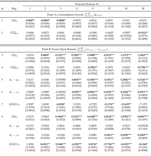
Table 5: Long-Horizon Regressions

Forecast HorizonH

# Reg. 1 2 3 4 8 12 16 24 Panel A: Consumption Growth,PH

i=1∆ct+i

1 caydt -0.0047* -0.0069* -0.0080* -0.0072 0.0014 0.0091 0.0141 0.0131

(0.0026) (0.0036) (0.0043) (0.0052) (0.0107) (0.0146) (0.0180) (0.0208) [0.0267] [0.0454] [0.0580] [0.0660] [0.0962] [0.1218] [0.1540] [0.2407] 2 cay\_{h t} 0.0040 0.0073 0.0081 -0.0008 -0.0290 -0.0425 -0.0597 -0.1312**

(0.0077) (0.0125) (0.0169) (0.0186) (0.0285) (0.0350) (0.037802) (0.0575) [0.0163] [0.0363] [0.0512] [0.0621] [0.0982] [0.1229] [0.1552] [0.2490]

Panel B: Excess Stock Returns,PH

i=1(rt+i−rf,t+i)

3 caydt 0.0214 0.0669* 0.1331*** 0.2302*** 0.5800*** 0.9233*** 1.1272*** 1.2443***

(0.0244) (0.0392) (0.0503) (0.0642) (0.1308) (0.1521) (0.1294) (0.1312) [-0.0069] [0.0034] [0.0175] [0.0438] [0.0809] [0.1639] [0.2379] [0.3824] 4 cay\_{h t} 0.0996 0.1534 0.1857 0.2003 0.2902** 0.2672 -0.0323 -0.7786***

(0.0732) (0.1032) (0.1290) (0.1495) (0.1371) (0.1967) (0.2269) (0.2311) [-0.0059] [0.0010] [0.0079] [0.0145] [0.0526] [0.1019] [0.1560] [0.3652] 5 dt−pt 0.0117 0.0348 0.055985 0.0657** 0.1585*** 0.1911** 0.2802*** 0.3126***

(0.0201) (0.0302) (0.0351) (0.0304) (0.0596) (0.0787) (0.0703) (0.0783) [-0.0072] [0.0031] [0.0134] [0.0214] [0.0429] [0.0783] [0.1537] [0.2783] 6 dt−et 0.0009 -0.0087 -0.020391 0.0391** 0.0941*** 0.1445*** 0.3224*** 0.2911***

(0.0138) (0.0306) (0.0397) (0.0180) (0.0360) (0.0393) (0.0360) (0.0420) [-0.0077] [-0.0035] [0.0047] [0.0251] [0.0554] [0.1202] [0.3018] [0.3788] 7 RRELt 0.5207 3.6982 6.0328* -3.5101 -4.7525 -13.174** -13.635** -7.1375

(2.1074) (2.7613) (3.1641) (2.7862) (5.2727) (5.7636) (6.8009) (8.0032) [-0.0041] [0.0086] [0.0219] [0.0149] [0.0243] [0.0685] [0.1038] [0.1633] 8 cayd_t 0.0179 0.0663 0.1404*** 0.2311*** 0.6340*** 1.0124*** 1.0701*** 0.8687***

(0.0312) (0.0443) (0.0523) (0.0808) (0.1524) (0.1489) (0.1413) (0.1695)

dt−pt 0.0173 0.0524 0.0814 0.0468 0.0859 0.0232 -0.0213 0.055328

(0.0267) (0.0438) (0.0516) (0.0363) (0.0740) (0.0828) (0.0758) (0.1126)

dt−et -0.0016 -0.0168 -0.0368 0.0181 0.0489 0.1011** 0.2959*** 0.2569***

(0.0146) (0.0332) (0.0429) (0.0189) (0.0416) (0.0431) (0.0389) (0.0499)

RRELt 2.4396 8.6521** 12.686*** -6.2927** -9.8741* -17.736*** -14.923*** -16.368*

(3.3107) (3.9507) (3.9608) (3.1389) (5.3831) (5.2806) (5.0180) (9.1167) [-0.0002] [0.0572] [0.1012] [0.0740] [0.1366] [0.2733] [0.4733] [0.5058]

This table reports estimates from the long-horizon regressions of accumulated consumption growth and accumulated excess stock returns oncay,d cay[hand the financial variables. We omit the

con-stants of all regressions. Reg. indicates the regressors included in each regression. The forecast horizon length is in quarters. White cross-section corrected standard errors are displayed in paren-thesis andR2are in brackets at the end of each regression. Statistics with(∗)are significant at 10%

level,(∗∗)at 5% and(∗ ∗ ∗)at 1%.

From Table 5 we may conclude that as a whole,_dcayis a much better predictor for both

consumption growth and excess returns thancay_dh. This means that if one wants to make

forecasts for any of those two variables in a panel, it is better to estimate a single cointe-grating vector for the entire panel and build acay with homogeneous coefficients rather

than estimate one cointegrating vector for each country and make an heterogeneouscay.

It is also clear that, comparing Table 4 with Table 5, dcay has a better performance

consumption growth, and for longer periods, its forecasting power is greater on excess returns. Thus we can see a strong persistence of dcay through time with an increasing of its forecasting power.

To check the effectiveness of_dcayas a predictor for excess returns, we add the financial

variables on the longer-term regressions. Row 5 reports regressions using the dividend yield as the sole forecasting variable and, considering theR2 of this regression set against

d

cay’s, we may say thatdcayis a much better predictor of excess returns thand−p, ignoring

the first period when both variables are not statistically significant. The same is true for the payout ratio, on 6. On the other hand, comparing theR2 of rows 3 and 7 we observe

a better fit withRRELas a predictor up to one year and withdcayso on.

Finally, on Row 8 we make the long-horizon regressions ondcayand all financial vari-ables. It is interesting to notice that the forecasting power of dividend yield has vanished when we use all variables together. This means that_dcay andRRELcapture all the effect

ofd−pover accumulated excess returns. From 3 to 8,_dcay’s coefficients stay almost the

same, so that it must not be considered replaceable by any financial variables. When com-paring rows 7 and 8 there is a considerable change inRREL’s coefficients. This is maybe

due to an omitted variable error in 7, which produces biased estimates. Then, on 8 we remain withcay and RREL as stronger predictors of excess returns over three quarters

and forth, and for longer horizons - more than three years -, the payout ratiod−emay be

considered a predictor as well. Comparing theR2’s from rows 3 and 8 we may say that it is worth including the financial variables together with _dcay when making forecasting

about excess returns.

From the theoretical framework we have seen that cay should Granger-cause asset

returns, once movements oncay were supposed to precede wealth variations caused by

asset returns fluctuations. Therefore, in order to improve our forecasting analysis, we perform Granger causality tests10_{checking ifdcayGranger-causes the excess stock returns.}

Indeed, with a lag length from four onward we reject at 1% the null of dcay does not

Granger-cause excess returns. This result is in line with the forecasting outcome from the previous regressions, which indicates thatdcay provides statistically significant informa-tion about future values of excess returns only after one year.

10_{The tests consist of running regressions with different lags,l, of the form}

(rt−rf,t) =α0+α1(rt−1−rf,t−1) +...+αl(rt−l−rf,t−l) +β1dcayt−1+...+βldcayt−l+ut

6 Robustness Checks

How robust are these forecasting results? On all previous regressions we have used the White cross-section correction to obtain standard errors robust to cross-section het-eroskedasticity and cross-section correlation. This approach however does not take into account any time-series dependence. Therefore, in this section we use another estimation method in order to correct the standard errors for both cross-section and serial correlation and heteroskedasticity.

We begin with a within transformation of the linear unobserved effects model we want to estimate. This transformation is obtained through a time demeaning of the panel equation, removing the individual specific effects (Wooldridge, 2010). Consider the linear model with unobserved effects forT periods andiindividuals

yit =ci+xitβ+uit. (13)

Then, by averaging this equation overt = 1, ..., T, we get to the cross section equation

yi =ci+xiβ+ui, (14)

where yi = T

−1PT

t=1yit, xi = T

−1PT

t=1xit and ui = T

−1PT

t=1uit. Subtracting equation

(13)from(14)for eacht, we obtain the transformed equation

¨

yit = ¨xitβ+ ¨uit, (15)

where y¨it ≡ yit−yi, ¨xit ≡ xit−xi,u¨it ≡ uit−ui and the specific effects removed. In our

case, the dependent variable would be the excess returns and the explanatory variables would be lagged_dcay and the lag of the financial variables.

With the fixed effects out of the picture, we follow the example given by Driscoll and Kraay (1998) in which there are cross-sectional and time dependence in the linear model. The procedure consists of taking the cross-sectional average of the variables in the model, which in our case are already time demeaned, reducing the panel to a single time series

1 N N X i=1 ¨

yit =

1 N N X i=1 ¨

xitβ+

1 N N X i=1 ¨

uit, (16)

˜

Then we apply the Newey and West (1987) consistent covariance matrix estimator11_{, in}

order to correct heteroskedasticity and serial correlation.

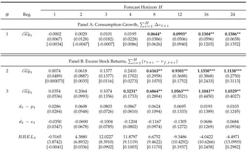
It is worth mentioning that this method comprises a broad class of spatial and tempo-ral dependence, requiring no prior knowledge of the exact form of the serial and cross-unit correlations. Table 6 shows the estimates of the log-term regressions obtained from the procedure described above, which we use to compare with the results of the previous section.

Table 6: Robustness Regressions

Forecast HorizonH

# Reg. 1 2 3 4 8 12 16 24 Panel A: Consumption Growth,PH

i=1∆ct+i

1 caydt -0.0002 0.0029 0.0101 0.0195 0.0644* 0.0993* 0.1304** 0.1586**

(0.0067) (0.0128) (0.0182) (0.0228) (0.0386) (0.0506) (0.0596) (0.0658) [-0.0034] [-0.0047] [-0.0007] [0.0086] [0.0626] [0.0940] [0.1203] [0.1352]

Panel B: Excess Stock Returns,PH

i=1(rt+i−rf,t+i)

2 caydt 0.0074 0.0618 0.1377 0.2410 0.6163** 0.9301** 1.1550*** 1.1138***

(0.0489) (0.0887) (0.1377) (0.1702) (0.2958) (0.3688) (0.3868) (0.2750) [0.000073] [0.0035] [0.0116] [0.0273] [0.1070] [0.1752] [0.2433] [0.3113] 3 caydt 0.0354 0.2064 0.1074 0.3231* 0.6864** 1.0563*** 1.1041** 1.0329**

(0.0536) (0.0993) (0.1356) (0.1733) (0.2884) (0.3521) (0.4450) (0.4027)

dt−pt 0.0286 0.0608 0.0803 0.0867 0.0624 0.0695 0.0193 0.0103

(0.0284) (0.0548) (0.0726) (0.0810) (0.1094) (0.1333) (0.1389) (0.1245)

dt−et -0.0350 -0.0690 -0.1004 -0.1204 -0.1167 -0.1305 0.0686 0.0684

(0.0347) (0.0678) (0.0785) (0.0802) (0.0974) (0.1272) (0.1269) (0.0934)

RRELt -0.5165 4.3880 12.0227 11.8797 6.6752 -9.3486 -4.0422 -4.4971

(3.8742) (6.8932) (8.3910) (9.1119) (9.4622) (10.4292) (10.6266) (13.0993) [-0.0041] [0.0336] [0.0902] [0.1003] [0.1170] [0.1937] [0.2458] [0.2982]

This table reports estimates from the long-horizon time series regressions of the average accumu-lated consumption growth and average accumuaccumu-lated excess stock returns ondcay’s and financial variables’ averages. There are no the constants on these regressions, since the fixed effects were eliminated after time demeaning. The Newey-West corrected standard errors are displayed in parenthesis andR2are in brackets at the end of each regression. Statistics with(∗)are

signifi-cant at 10% level,(∗∗)at 5% and(∗ ∗ ∗)at 1%.

Analyzing Table 6, we notice from Rows 1 and 2 that _dcay is able to predict both

con-sumption growth and excess returns only in the long run, but its forecasting power is higher for excess returns as well as its impact. Furthermore, when we make the regres-sions with all variables together,_dcayis the sole statistically significant variable.

Considering the accumulated consumption growth, we can see that Panel A has con-siderably changed from Table 5 to Table 6. On the first, dcay is a statistically significant

predictor for consumption growth over short horizons, while on the latter, this variable starts being significant only after two years. Hence, with such different results, there is no confirmation about the robustness ofdcay as a consumption growth predictor.

Comparing Row 3 from Table 5 and Row 2 from Table 6, it is clear that dcay may be used as a predictor for excess returns over short horizons only if one is applying the first estimation method - LSDV with White cross-section corrected standard errors. However, over two years, both methods present almost the same results for the impact ofcay_dover

excess returns and for its forecasting power, which supports the robustness of this vari-able as a predictor for excess returns over higher period lengths.

The last row of both tables show that together with all financial variables, dcay is a

robust predictor of excess returns from two years onward, since that their coefficients and significance level present negligible differences. On the other hand, the forecasting power ofRRELanddt−ethave disappeared on the robustness regressions, suggesting

that they are not as strong as dcay for predicting returns. In addition and in contrast to Table 5, when comparing theR2’s from Rows 2 and 3 of Table 6 we see that the financial

variables can be considered disposable as predictors for excess returns.

We may conclude from this robustness analysis12_{and from the long-term regressions}

of the last section that_dcayshould in fact be considered a strong predictor for future excess

stock returns over long horizons - more than one year. It is the only predicting variable that survived our robustness tests. In addition, scanning theR2’s from Tables 5 and 6 we

may say that both estimation methods have almost the same forecasting power for excess returns, with respect todcay, as a whole.

7 Out-of-Sample Tests

Several forecasting researches indicate that some variables with strong predictive power in-sample do not necessarily perform out-of-sample forecasts that well. This is probably due to "look-ahead" bias when coefficients are estimated using the full sample. We ad-dress this problem by making some nested and non-nested out-of-sample forecast com-parisons, analyzing the mean-squared error (MSE) of one-quarter-ahead panel forecasts.

Both nested and non-nested models are first estimated using data from the first quarter of 1981 to the first quarter of 2004 and then recursively re-estimated adding one quarter at a time and calculating one-step-ahead forecasts until the fourth quarter of 2013. In order to remain with just one MSE for the panel, we compute the out-of-sample forecasting error for each country and take the trace of the matrix of cross product of this errors,

12_{We have also performed this robustness exercise without the within transformation, such that the fixed}

effects remained in the model when we took the cross-sectional average and the intercept of the time series was an average of this fixed effects. The results present slightly differences on coefficients andR2and bring

obtaining a sum of the MSE’s.

We analyze the MSE of models using either dcay, with cointegrating parameters esti-mated in the full sample, orreest_dcay, with the parameters re-estimated every period. The

former case gives an idea of the results if one used the existing estimates of the parame-ters and faced the same distribution of data, while the latter is a more realistic scenario using only data available at the time of forecast.

This exercise is done not only for one-step-forward excess returns (rt+1 −rf,t+1), but

also for two years accumulated excess returns (P8

i=1(rt+i −rf,t+i)), since the results of

the last two sections indicate that in-sampledcayshould not be a good predictor

one-step-forward but present strong and robust forecasting power two years onward. Therefore, we would be able to evaluate the impact of dcay over the MSE of excess returns with different period lengths.

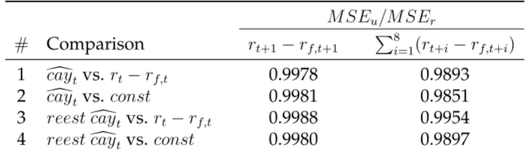
On the nested regressions, we begin with two parsimonious models, thelagged bench-markusing just one-period lagged value of excess return as a predictors and theconstant

benchmark with a constant as the sole explanatory variable assuming constant expected

returns. Then we make the comparisons by augmenting the benchmarks with the one-period lagged value ofdcay. The results of this nested comparisons are presented on Table

7.

Table 7: Out-of-Sample Nested Comparisons

M SEu/M SEr

# Comparison rt+1−rf,t+1 P8i=1(rt+i−rf,t+i)

1 dcaytvs. rt−rf,t 0.9978 0.9893

2 dcay_tvs. const 0.9981 0.9851

3 reest_dcaytvs. rt−rf,t 0.9988 0.9954

4 reestdcaytvs. const 0.9980 0.9897

This table shows the results of the nested comparisons, displaying the MSE ratio from the un-restricted model, which includesdcay, over the restricted model with either lagged excess returns (rt−r_f,t) or a constant (const) as the sole predictor. The first column with values refers to

one-quarter-ahead excess returns forecasts and the second one refers to two years accumulated excess returns predictions. The first two rows are computed withdcayestimated from the full sample and the last two with its parameters recursively re-estimated (reestcay).d

The column of one-step-ahead excess returns indicates that dcay and its re-estimated version have almost the same impact over the MSE ratio when added to the constant benchmark and to the lagged benchmark. On the other hand, for two years accumulated excess returns,_dcay reduces the MSE by more than the model that usesreest_dcay. We can

also see from the second column of MSE values that the gains from augmenting the mod-els with both_dcay’s are greater on the constant benchmark than on the lagged benchmark.

Next, we extend our analysis by making nonnested forecasts to see if dcay and its

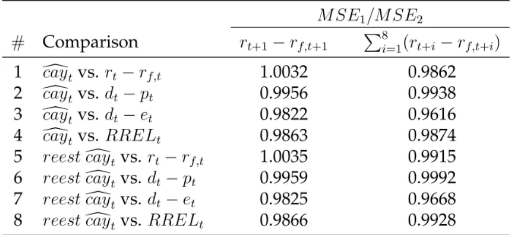
re-estimated version as sole predictive variables exhibit more information and smaller MSE relatively to the models with financial variables - dividend yield, payout ratio and the rel-ative bill rate - and lagged excess returns as the sole predictor. The results from nonnested comparisons are given in Table 8.

Table 8: Out-of-Sample Nonnested Comparisons

M SE1/M SE2

# Comparison rt+1−rf,t+1 P8i=1(rt+i−rf,t+i)

1 dcaytvs. rt−rf,t 1.0032 0.9862

2 dcay_tvs. dt−pt 0.9956 0.9938

3 _dcaytvs. dt−et 0.9822 0.9616

4 dcaytvs. RRELt 0.9863 0.9874

5 reest_dcay_tvs. rt−rf,t 1.0035 0.9915

6 reest_dcaytvs. dt−pt 0.9959 0.9992

7 reestdcaytvs. dt−et 0.9825 0.9668

8 reestdcaytvs. RRELt 0.9866 0.9928

This table reports the results of nonnested comparisons, displaying the MSE ratio from the first model, with eithercaydorreestdcayas the sole predictor, over the second model, with financial variables or lagged excess returns. Once more, the first column with values refers to one-quarter-ahead excess returns forecasts and the second one refers to two years accumulated excess returns predictions. The first four rows are computed withcaydestimated from the full sample and the last two with its parameters recursively re-estimated.

Compared to the financial variables, dcay produces superior forecasts regardless of

whether its coefficients are re-estimated or whether we want to predict the next quar-ter or two years accumulated excess returns. The strength of _dcay as a predictor may be

noticed specially with regard to the payout ratio,d−e. However, when making forecasts

over one quarter ahead, both_dcayandreest_dcayproduce higher MSE’s in relation to lagged

excess returns.

Except for RREL, the impact of dcay and reest dcay over the MSE ratio is greater for

two years accumulated excess returns. At this time length, the forecasting power ofdcay

re-estimated version, as one would expect.

All of these findings indicate that for longer horizonsdcayproduces forecasts superior to any of the competitor models. In addition, _dcay should be included together with a

constant or lagged excess returns to improve the forecasts, regardless of the time horizon. We conclude that these out-of-sample results are consistent with the in-sample results as a whole.

8 Conclusion

Our work here was to settle the link between the consumption-wealth ratio and expected stock returns through a panel approach, estimating the cointegrating residual from the shared trend among consumption, asset wealth and labor income, cay, and verifying

its forecasting power over stock returns. According to the theoretical framework, when agents expect higher asset returns in the future they increase current consumption in or-der to smooth out their purchasing power, which leads to a detachment of consumption from its shared trend with asset wealth and labor income. Therefore, movements oncayt

should forecast future asset returns.

Using quarterly data from 1981 to 2014, we set a panel for G7’s countries and, af-ter testing the cointegrating relationship between consumption, asset wealth and labor income, we estimate cay with a VEC. Then, using our panel data, we make

one-step-forward forecasts as well as long horizon regressions to investigate the power of_dcay as a

predictor for excess stock returns. Neither_dcay nor the financial variables that we include

on regressions are able to predict excess returns one quarter ahead. Nevertheless, the forecasting power ofdcaysurprisingly increases as the forecast horizon becomes longer. In

fact, the impact ofdcayover future excess returns starts being statistically significant over

three quarters and increases together withdcay’s forecasting power thereafter.

On our robustness analysis, we study another way of estimating the forecasting pa-rameters and correcting standard errors. Once more, none of the predictive variables is capable of predicting excess returns one quarter ahead. However,dcayexhibits substantial forecasting power at horizons ranging from two years and so on, and among the financial variables, is the only predictor which outlasts our robustness exercise.

In addition, we perform nested and nonnested out-of-sample excess returns forecasts adding one quarter at a time and recursively estimating the predictors parameters. On the nested comparisons,dcay has improved the forecasting performance for both constant

the MSE of forecasts with dcay as the sole predictive variable is consistently lower than the MSE of prediction with the financial variables. However, for one-quarter-ahead fore-casts on these nonnested comparisons, the performance ofcay_dfalls short of the predictive

power of lagged excess returns, although this effect is reversed when making two-year-ahead predictions.

We may conclude from our analysis that, when estimated with panel data, cay is

in-deed a strong and robust predictor of future excess returns from two years onward. One possible explanation to this delayed response is that we could be estimating a long-run equilibrium tendency and that cay is not able to capture short-term volatility of excess

returns.

References

Arellano, M. (1987, November). Computing Robust Standard Errors for Within-Groups Estimators. Oxford Bulletin of Economics and Statistics 49(4), 431–34.

Campbell, J. Y. (1996, April). Understanding Risk and Return. Journal of Political

Econ-omy 104(2), 298–345.

Campbell, J. Y. and J. H. Cochrane (1999, April). By force of habit: A consumption-based explanation of aggregate stock market behavior.Journal of Political Economy 107(2), 205–

251.

Campbell, J. Y. and N. G. Mankiw (1989, Jan-Jun). Consumption, Income and Interest Rates: Reinterpreting the Time Series Evidence. InNBER Macroeconomics Annual 1989,

Volume 4, NBER Chapters, pp. 185–246. National Bureau of Economic Research, Inc.

Campbell, J. Y. and R. J. Shiller (1988, July). Stock Prices, Earnings, and Expected Divi-dends. Journal of Finance 43(3), 661–76.

Driscoll, J. C. and A. C. Kraay (1998, November). Consistent Covariance Matrix Estima-tion With Spatially Dependent Panel Data. The Review of Economics and Statistics 80(4),

549–560.

Engle, R. F. and C. W. J. Granger (1987, March). Co-integration and Error Correction: Representation, Estimation, and Testing. Econometrica 55(2), 251–76.

Fama, E. F. and K. R. French (1988, October). Dividend yields and expected stock returns.

Journal of Financial Economics 22(1), 3–25.

Fisher, R. A. (1932). Statistical Methods for Research Workers(4th ed.). Edinburgh.

Gao, P. P. and K. X. Huang (2008, May). Aggregate Consumption-Wealth Ratio and the Cross-Section of Stock Returns: Some International Evidence. Annals of Economics and

Finance 9(1), 1–37.

Hodrick, R. J. (1992). Dividend Yields and Expected Stock Returns: Alternative Proce-dures for Interference and Measurement. Review of Financial Studies 5(3), 357–386.

Ioannidis, C., D. Peel, and K. Matthews (2006, June). Expected stock returns, aggre-gate consumption and wealth: Some further empirical evidence. Journal of

Johansen, S. (1991, November). Estimation and Hypothesis Testing of Cointegration Vec-tors in Gaussian Vector Autoregressive Models. Econometrica 59(6), 1551–80.

Judson, R. A. and A. L. Owen (1999, October). Estimating dynamic panel data models: a guide for macroeconomists. Economics Letters 65(1), 9–15.

Lamont, O. (1998, October). Earnings and Expected Returns. Journal of Finance 53(5),

1563–1587.

Lettau, M. and S. Ludvigson (2001, June). Consumption, Aggregate Wealth, and Expected Stock Returns. Journal of Finance 56(3), 815–849.

Lettau, M. and S. C. Ludvigson (2004, March). Understanding Trend and Cycle in As-set Values: Reevaluating the Wealth Effect on Consumption. American Economic

Re-view 94(1), 276–299.

Maddala, G. S. and S. Wu (1999). A comparative study of unit root tests with panel data and new simple test.Oxford Bulletin of Economics and Statistics, Special Issue 61, 631–652.

Newey, W. K. and K. D. West (1987, May). A Simple, Positive Semi-definite, Heteroskedas-ticity and Autocorrelation Consistent Covariance Matrix. Econometrica 55(3), 703–08.

Nickell, S. J. (1981, November). Biases in Dynamic Models with Fixed Effects.

Economet-rica 49(6), 1417–26.

Nitschka, T. (2010, November). International Evidence for Return Predictability and the Implications for Long-Run Covariation of the G7 Stock Markets. German Economic

Re-view 11, 527–544.

Pesaran, M. H. and A. Timmermann (1995, September). Predictability of Stock Returns: Robustness and Economic Significance. Journal of Finance 50(4), 1201–28.

Runkle, D. E. (1991, February). Liquidity constraints and the permanent-income hypoth-esis : Evidence from panel data. Journal of Monetary Economics 27(1), 73–98.

Tsuji, C. (2009, August). Consumption, Aggregate Wealth, and Expected Stock Returns in Japan. International Journal of Economics and Finance 1(2), 123–133.

Wooldridge, J. M. (2010, July). Econometric Analysis of Cross Section and Panel Data,

Vol-ume 1 ofMIT Press Books. The MIT Press.