Elcyon Caiado Rocha Lima**
Summary: 1. Introduction; 2. The NAIRU and the natural rate of unemployment; 3. The data and the estimated models; 4. The estimation procedures; 5. The model’s estimation results; 6. The
estimated NAIRU and the response of ∆π to cyclical
unemploy-ment; 7. Conclusions.
Keywords: time-varying NAIRU, Markov switching, Phillips curve, Kim filter, unobserved-components model.
JEL codes: C22; E32.
This paper estimates the Brazilian NAIRU (Nonaccelerating In-flation Rate of Unemployment) and investigates several empirical questions: the stability of coefficients of the Brazilian price Phillips curve, the behavior of the NAIRU along time, and error bands for the NAIRU. This article innovates, with respect to previous re-search work done for Brazil, because it estimates error bands for the NAIRU and adopts econometric models that, in our judgment, deal more adequately with the still recent instability of the Brazil-ian economy. We estimate two different state-space models: one with a time-varying NAIRU and another in which the NAIRU is changing over time according to a hidden Markov chain specifica-tion.
The study presents some new evidence on several questions. It shows that while the slope of the Brazilian price Phillips curve is stable the NAIRU has not been stable. It concludes that there is a statistically significant relationship, with correct sign, between deviations of unemployment from the NAIRU and inflation. It also shows that, after the second semester of 1995, there is no significant evidence that the NAIRU has been different from the observed unemployment rate.
Neste artigo estima-se a NAIRU (a taxa de desemprego que mant´em
*This paper was received in Apr. 2002 and approved in Dec. 2002. The author thanks
Christopher C. Sims, whose lectures at Yale have inspired this paper, Eust´aquio J. Reis, Paulo M. Levy and three anonymous referees for their comments on an initial version of this article, and the CNPq for the financial support given to this research during the postdoctoral program at Yale University , in the United States.
est´avel a taxa de infla¸c˜ao) do Brasil e investiga-se diversas quest˜oes emp´ıricas: a estabilidade dos coeficientes da Curva de Phillips (para pre¸cos) brasileira , o comportamento da NAIRU ao longo do tempo, e os intervalos de confian¸ca para a NAIRU.
O presente trabalho inova, em rela¸c˜ao aos anteriores, ao adotar modelos econom´etricos que, acredita-se, s˜ao mais adequados para lidar com as instabilidades defrontadas pela economia brasileira em per´ıodo recente. Estimam-se dois modelos diferentes em espa¸co-de-estados: um com uma NAIRU que muda ao longo do tempo e outro no qual a NAIRU muda, ao longo do tempo, de acordo com a especifica¸c˜ao de uma cadeia de Markov oculta.
Obt´em-se novas evidˆencias sobre diversas quest˜oes emp´ıricas. Mos-tra-se que a inclina¸c˜ao da Curva de Phillips do Brasil ´e est´avel mas que a NAIRU brasileira vem se alterando ao longo do tempo. Conclui-se que existe uma rela¸c˜ao estatisticamente significante, e com o sinal correto, entre os desvios da taxa de desemprego em rela¸c˜ao `a NAIRU e a taxa de infla¸c˜ao. No entanto, devido `a impre-cis˜ao das suas estimativas, n˜ao h´a evidˆencia significativa de que a NAIRU, depois do segundo trimestre de 1995, tenha sido diferente da taxa de desemprego observada.
1.
Introduction
In this article we estimate the Brazilian Phillips curve aiming to obtain the Nonaccelerating Inflation Rate of Unemployment (NAIRU) for Brazil. We investi-gate the stability of coefficients of the Brazilian Phillips curve and the relationship between the rate of inflation and the deviation of the observed rate of unemploy-ment from the NAIRU. We also estimate error bands for the NAIRU in order to determine whether there is any significant difference between the NAIRU and the observed unemployment rate.
plans point in the direction of using models that allow for large breaks and frequent alternations of the states of the economy.
Portugal et al. (1999) estimate two different models for the Brazilian NAIRU. The first model is a traditional Phillips curve with constant intercept, autoregres-sive residuals and dummies to allow for structural breaks. The second model is a univariate structural model with trend and cycle, Harvey (1989), in which the NAIRU is defined as the trend component. The definition of the NAIRU, used in the second model, is questionable and in the literature (Staiger et al., 2001, Cogley and Sargent, 2001, Hall, 1999) there is a distinction between the natural rate of unemployment, usually defined as the unemployment trend, and the NAIRU.
In Corseuil et al. (1996) there are no calculations for the NAIRU but there is a careful analysis of the components of unemployment (trend and cycle), for the main metropolitan regions of Brazil. They test the relative importance of aggregate and regional shocks in the determination of unemployment and conclude that there is evidence in favor of a strong influence of aggregate factors.
We believe that the structural breaks in the models for the Brazilian NAIRU cannot be dealt with by models with dummies and autoregressive residuals (Por-tugal et al., 1999), thresholds [TAR model, (Tong, 1990)] or with time-varying smooth transitions between states [STAR model, Ter¨asvirta (1994) or TV-STAR model, Lundbergh et al. (2002)]. Fortunately, since the beginning of the ’90s there has been a variety of theoretical developments in time series analysis that enable us to extract information from data even when instabilities, like the ones observed for Brazilian data, are present [Hamilton (1989); Kim (1994); Kim and Nelson (1999); Sims (1999); Sims and Zha (2002)]. These developments allow us to deal with a larger set of data.
Our research innovates, when compared to other research work done for Brazil, because it adopts some of these developments which, in our view, deal more ade-quately with abrupt structural breaks in the model’s equation and frequent alter-nations of the states of the economy. We estimate two different models to calculate the natural rate of unemployment and its confidence interval: one model with a time-varying NAIRU and another model in which the NAIRU is changing over time according to a hidden Markov chain specification. The first model allows for the presence of ARCH residuals; the second model allows for persistent het-eroscedasticity1 as well as a richer pattern of time variation for the NAIRU. We
1Sims (1999), using monthly data on a short term interest rate and a commodity price index
could not reject the absence of ARCH residuals in the first model under the main-tained hypothesis of a time-varying NAIRU. Under the specification for the second model, we could not reject the presence of both Markov-switching heteroscedas-ticity and a time-varying NAIRU. A detailed description of both models and of the estimation methods can be found in Kim and Nelson (1999). The models were estimated using quarterly data for the average rate of open unemployment in six Metropolitan Regions and for the rate of inflation measured by the national consumer price index (INPC) in eleven Metropolitan Regions (including the six regions where unemployment is measured), both collected by IBGE for the period 1982:1 – 2001:4.
Following Staiger et al. (2001), the recent theories that have been proposed to explain the relationship between inflation and unemployment can be classified into two groups: theories in which “the Phillips curve is alive and well but...” and those that proclaim the “the Phillips curve is dead”. The theories in the first group ((Staiger et al., 1997, 2001); Gordon (1982, 1997, 1998);King and Watson (1994); Blanchard and Katz (1997)) conclude that the Phillips curve continues to have the same negative slope but it has been shifting. A good survey of these theories can be found in Katz and Krueger (1999). The theories in the second group interpret the recent events as a change in the slope of the Phillips curve (Akerlof et al. (1996, 2000) ; Taylor (2000)). For Brazil, the most recent study (Portugal et al., 1999) can be classified in the first group. This study did not find evidence that the slope of the Brazilian Phillips curve has changed, but it could not reject that the curve has been shifting.
The article is organized as follows: In section 2, we describe the data used, how the monthly data were transformed into quarterly data and the estimated models; in section 3, we present the estimation procedures adopted, and in the appendix, we describe the Kim filter and its use in the estimation of one of the models; in section 4, we show the estimation results and discuss some statistical tests; in section 5, we conclude.
2.
The NAIRU and the Natural Rate of Unemployment
For many researchers, the NAIRU is a synonym for the natural rate of unem-ployment. However, we find it convenient to separate these two concepts, just as do many others (Staiger et al. (2001), Cogley and Sargent (2001), Hall (1999)).
The idea of a natural rate of employment was first proposed in Friedman’s
(1968) presidential address to the American Economic Association: “The natural rate of unemployment is the level which would be ground out by the Walrasian system of general equilibrium equations, provided that there is embedded in them the actual structural characteristics of the labor and commodity markets, includ-ing market imperfections, stochastic variability in demands and supplies, the cost of gathering information about job vacancies and labor availabilities, the costs of mobility, and so on”. The main point of Friedman’s address was to argue that there was no permanent (long-run) tradeoff between inflation and unemployment. His definition does not require the existence of a short-run inflation-unemployment tradeoff. Therefore, there is a natural rate of unemployment, even in the absence of any short-run unemployment-inflation tradeoff. Besides, as pointed out by Roger-son (1997), his definition is not inconsistent with the natural rate of unemployment being equal to the low frequency (trend) movements in unemployment.
The NAIRU concept, on the other hand, needs the view (a view which is very prominent among central bankers and monetary economists) that there is a short-run inflation-unemployment tradeoff. Even though, for many economists, the existence of this short-run tradeoff is purely speculative, its existence is one of the most enduring ideas in macroeconomics: shocks in monetary policy push inflation and unemployment in opposite directions in the short run. If this trade-off is admitted, there must be some level of unemployment (NAIRU) consistent with constant inflation. Therefore, if a contractionary shock in monetary policy increases unemployment above the NAIRU, the inflation rate will decrease, and if an expansionary monetary shock decreases the unemployment rate below the NAIRU, the inflation rate will increase.
One simple model for the relationship between unemployment (u), inflation change (∆π) and the NAIRU (¯u) is given by ∆πt=β(ut−u¯)+ǫt=−βu¯+βut+ǫt= α+βut+ǫt, where α=−βu¯ and ǫt is the error term. In this model the NAIRU
Figure 1
Inflation Change x Unemployment
Dp= -0.6873*U + 3.7 (0.549) (3.1)
R2= 0.0197
NAIRU= 5.4%
-50.00% -40.00% -30.00% -20.00% -10.00% 0.00% 10.00% 20.00%
2% 3% 4% 5% 6% 7% 8% 9%
Open Unemployment
Dp
The problem with this estimate of the NAIRU is that it does not control for other factors that may affect the relationship between inflation and unemploy-ment, such as inflation stabilization plans, seasonal effects and lagged effects of unemployment and inflation. This lack of control for other factors may explain why both coefficient of the regression line are not significantly different from zero. Figure 2 is identical to figure 1 but shows data from 1995:1-2001:IV, which is the period after the Real Plan with much lower inflation. Figure 2 shows no evident relationship between inflation change and unemployment. One possible explanation is the absence of the short-run tradeoff between inflation and unem-ployment under low inflation. However, we will show that this relationship can still be recovered from the most recent data if a more complicated model, one with time-varying parameters, is adopted.
Figure 2
Inflation Change x Unemployment
-1.5% -1.0% -0.5% 0.0% 0.5% 1.0%
2% 3% 4% 5% 6% 7% 8% 9%
Open Unemployment
It should be emphasized that the models used to estimate the NAIRU need more than the existence of the short-run tradeoff. They need the notion that monetary policy affects the price level by first affecting unemployment, which, then, via a Phillips Curve, affects inflation. In the next section we describe the specification adopted to identify the Brazilian NAIRU.
3.
The Data and the Estimated Models
The basic data comprise the national consumer price index (INPC) of IBGE from 1981:12 to 2002:01 and the average rate of open unemployment of IBGE from 1982:1 to 2001:12. These monthly data were averaged into quarterly data resulting in a sample size of 80 observations. The model was estimated using only quarterly data, from the first quarter of 1982 to the last quarter of 2001. The monthly data was transformed into quarterly data as follows:
πt= (1/3).log(Pt,f/Pt−1,f) = monthly geometric average of the quarterly rate
of inflation;
Pt,f = centered INPC ( national consumer price index) of IBGE for the last
month of quarter t;
Ut = quarterly average of the monthly average rate of open unemployment of
IBGE.
3.1
The basic model
Our basic model for the relationship between the change of the rate of inflation and the rate of unemployment can be represented by the following equations:2
∆πt=µt+
3
s=1
βst(ut−s−u¯t−s) +Ztγt+ǫt (1)
and
3
s=0
µt+s= 0 (restriction that allows for the identification ofut)3 (2)
2This is the standard specification used for the Phillips curve (Staiger et al. (1997, 2001),
where
µt=α0t+α1tD1t+α2tD2t+α3tD3t (3)
Dit = seasonal dummy of quarteri;
ut−1 = NAIRU att−1;
Zt = is a row vector of control variables with the two first lags of ∆πt;4
ǫt∼N(0, σ2)
Equation (1) can also be represented in the following form:
∆πt=µt+
3
s=1
βstut−s−
2
s=1
ξst∆¯ut−s−ξ0tu¯t−1+Ztγt+ǫt (1’)
whereξ1t=−β1t−β2t, ξ2t=−β3t, ξ0t=β1t+β2t+β3tand ∆¯ut−s= ¯ut−s−u¯t−s−1. If the NAIRU slowly changes over time then 2
s=1
ξs∆¯ut−s ∼= 05 Furthermore,
3
s=0
µt+s= 0 implies that α0t=−α1t/4−α2t/4−α3t/4. Therefore,
∆πt =
3
s=1
(Dst−1/4)αst+
3
s=1
βstut−s−
2
s=1
ξst∆¯ut−s−ξ0tu¯t−1+Ztγt+ǫt
∼
= 3
s=1
(Dst−1/4)αst+
3
s=1
βstut−s−ξ0tu¯t−1+Ztγt+ǫt
∆πt = β0t+
3
s=1
(Dst−1/4)αst+
3
s=1
βstut−s+Ztγt+ǫt (4)
4We use two lags of ∆πbecause the basic model is one of the equations of a three lags VAR
on inflation and unemployment in which the sum of coefficients of lagged inflation is equal to 1. Sargent (1971) has pointed out that, under rational expectations, this restriction is only valid if inflation has a unit root. We tested and did not reject that inflation in Brazil is I(1). This restriction is necessary for the existence of the NAIRU and implies the absence of any long-run trade off between inflation and unemployment.
5We are using here the same restriction adopted by Staiger et al. (2001). Alternatively, this
restriction can be justified, if the initial model is similar to the one in King et al. (1995) and is given by ∆πt=µt+
3
s=1
whereβ0t≡ −ξ0tu¯t−1≡ −(β1t+β2t+β3t)¯ut−1.
If (β1t+β2t+β3t)<0 andβ0t>0, for allt, then we can obtain ¯ut−1 estimating the model and using the last equation:
¯
ut−1=−β0t/(β1t+β2t+β3t) (5)
The inflation stabilization plans adopted by Brazil (Cruzado (1986:1 and 1986:2), Bresser (1987:3), Ver˜ao (1989:1), Collor I (1990:2), Collor II (1991:2) and Real (1994:3)) have produced, in the quarters of their implementation, an abrupt reduction of the rate of inflation. To deal with these shocks, interventions were made in the model at each quarter of implementation of each stabilization plan. The basic model with interventions at each stabilization plan is described by the following equation:
∆πt=β0t(1 +θtτ) +
3
s=1
[Dst−(1/4)∗(1 +θtτ)]αst+
3
s=1
βstut−s+Ztγt+ǫt (6)
θtτ = 0, if there was no stabilization plan at quartert;
θtτ = θτ = nonlinear intercept intervention parameters when stabilization plan
“τ” happens at periodt
τ = 1 (Cruzado and Collor II Plans),τ = 2 (Bresser and Ver˜ao Plans),τ = 3 (Collor I and Real Plans)
To simplify the description of the model we summarize the representation of the model as follows:
Let
yt= ∆πt;xt=(1 +θtτ) (D1t−(1/4) (1 +θtτ)) (D2t−(1/4) (1 +θtτ))
(D3t−(1/4) (1 +θtτ))ut−1 ut−2 ut−3 Zt
βt∗ = [β0tα1tα2tα3tβ1tβ2tβ3tγt]
therefore the model can be represented, in a compact form, by
yt=xt(θtτ)βt∗+ǫt (7)
parameters. To deal with possible structural breaks we estimate two different versions of the above model: the TVP model (which allows for parameter change over time and ARCH residuals); the MSR model (which allows for parameter change over time and Markov-switching regimes).
3.2
The TVP and the MSR models
The TVP Model
The TVP model is a state-space model with ARCH residuals and is a simplified version of the model proposed by Harvey et al. (1992):
yt=xt(θtτ)βt∗+ Λǫ∗t +ǫt, measurement equation (8)
βt∗=βt∗−1+ωttransition equation (9)
ǫt∼N
0, σ2
, ωt∼N(0,Q) and ǫt∗/ψt−1 ∼N(0, h1t)
whereψt−1 = [yt−1, yt−2, ...., y1] , information available up to timet−1; Λ, ǫ∗t and σ are scalars and Q is, by hypothesis, diagonal and 9 x 9.
The ARCH effect is introduced through the scalar residualǫ∗
t. The variance of ǫ∗t is given by
h1t= 1 +γ0ǫ∗t−21 (10)
The MSR Model
The MSR model is a state-space model with a Markov-switching regime. It is a simplified version of the model suggested by Kim and Nelson (1999):
yt=xt(θtτ)βt∗+ǫt, measurement equation (11)
βt∗ =β∗t−1+ωt, transition equation (12)
The subscript St denotes thatσ2 and the parameters at the diagonal of ma-trixQtake values that depend on a discrete, nonobserved variable, that follows a Markov-switching process with 2 different states (regimes). The transition proba-bilities are given by
P=
p11 p12
p21 p22
(13)
where, piJ = probability of stateJ, at period t, given stateiat period t−1 and
2
J=1piJ = 1, i= 1,2 (14)
4.
The Estimation Procedures
4.1
The TVP model estimation procedure
Harvey et al. (1992) substitute the ǫ∗t−21 variable in equation (10) , which is nonobserved, by its conditional expectation,h1t= 1 +γEǫt∗−21/ψt−1. Therefore, the algorithm is an approximation. To get E
ǫ∗t−21/ψt−1 , Harvey, Ruiz and Sentana augmented the original state vector in the transition equation (9) in the following way:
βt∗
ǫ∗t
=
I9 0
0 0
βt∗−1
ǫ∗t−1
+
I9 0
0 1
ωt ǫ∗t
where I9 is the identity matrix with 9x9 dimension. Therefore, the measurement equation (8) is replaced by
yt= [xt(θt) Λ]
β∗t
ǫ∗t
+ǫt
It is not hard to show that
E
ǫ∗t−21/ψt−1=Eǫ∗t−1/ψt−12+E ǫ∗t−1−E(ǫ∗t−1/ψt−1)2
The two expectations at the right-hand side of the last equation can be com-puted, recursively, using the Kalman filter. The first expectation is equal to the recursive estimation of the second element of the state vector (ǫ∗
Given the intercept intervention parametersθτ[τ = 1,2 and 3], σ,Λ, γ0andQ, it is possible to obtain the model’s likelihood value andβt∗through the Kalman Fil-ter recursions. That is, we can concentrate the likelihood with respect toβt∗, using the Kalman filter and, with the help of a numerical optimization routine, estimate
the value of the other parameters
θτ(τ = 1,2 and 3),σ,Λ, γ0 and the elements
at the diagonal of matrixQ
that maximizes the likelihood.
To arrive at a more parsimonious model the following restrictions were imposed a priori:
Q(2,2) =Q(3,3) =Q(4,4), equality between parameters, at the diagonal of ma-trix Q, which controls for the time change of seasonal dummies coefficients;
Q(5,5) =Q(6,6) =Q(7,7), equality between parameters, at the diagonal of ma-trix Q, which controls for the time change of lag unemployment coefficients;
Q(8,8) = Q(9,9), equality between parameters, at the diagonal of matrix Q, which controls for the time change of lag ∆πt coefficients.
With these restrictions matrixQ has only 4 unknown parameters. Therefore, the TVP model has, if we exclude the parameters ofβ∗t from the counting, a total of 10 parameters to be estimated. In section 5.1 we describe how, departing from this more general model and using a few statistical tests, we are able to reduce, from 10 to 5, the number of parameters to be estimated.
4.2
The MSR model estimation procedure
We adopt the same restrictions for the MSR model – on the parameters of the diagonal of matrix Qi (state i = 1,2) – which were imposed on the TVP
model in section 3.1. Furthermore, equation (15) shows that we can estimate onlyp11andp21in order to obtain the entire matrix P. Therefore, givenp11,p22,
θτ(τ = 1,2,3), σi(the measurement equation residual’s standard deviation at state i, i = 1,2), and the 4 parameter in the diagonal of matrix Qi, at each state, we
can use Kim’s filter and smoothing algorithm (Kim and Nelson, 1999) to estimate β∗t and calculate the value of the likelihood of the MSR model. The Kim’s filter obtains the nonlinear mapping from the hyperparameters (σi andQi;i= 1,2), the
parameters inP, and the intervention parameters θτ(τ = 1,2,3) to the likelihood
value. We use this mapping to estimate the likelihood maximizing values of these hyperparameters and parameters using a numerical optimization routine. That is, the likelihood can be concentrated with respect toβ∗t making it easier to estimate
p11, p22, θτ(τ = 1,2,3) , σ1 , σ2 and the parameters at the diagonal of matrix Q, at each state, with the help of a numerical optimization routine. The results of this estimation are presented in section 5.2.
The MSR model has 15 parameters to be estimated through the numerical optimization routine6. Therefore, there is an excessive number of parameters. We show, in the next section, how departing from this more general model and using a few statistical tests, we impose some restrictions and end up with a model with only 8 parameters to be estimated through the numerical optimization routine.
5.
The Model’s Estimation Results
The two models were estimated using computer programs developed with the help of the “Matlab” software. The log likelihood for the two models, and for a variety of alternative hypothesis, is presented in table 1.
6The parameter of β∗
t do not enter explicitly in the numerical optimization routine. They
Table 1
Log likelihood and alternative hypothesis
TVP Model
Initial Model (10 parameters) 112.07
Simplified Models (Q(j, j) = 0, forj= 1,Λ = 0 andγ0= 0)
Q(1,1)= 0 (5 parameters) 111.43 (selected model)
Q(1,1) = 0 (4 parameters) 107.87
MSR Model
Initial Model (15 parameters) 121.27
Simplified Models (Qi(j, j) = 0, forj= 1 andi= 1,2)
Q1(1,1)=Q2(1,1) (regime dependent) (9 par.) 121.26 Q1(1,1) =Q2(1,1) (regime independent) (8 par.) 121.06
Q1(1,1)= 0 andQ2(1,1) = 0 (regime dependent) (8 par.) 121.09 (selected model) Q1(1,1) = 0 andQ2(1,1)= 0 (regime dependent) (8 par.) 119.33
Q1(1,1) =Q2(1,1) = 0 (regime independent) (7 par.) 113.14
Note : the parameter count, in this table, does not include the parameters ofβ∗t
(β∗t has 9 other parameters)
5.1
The TVP model results and the stability of coefficients of the
brazilian price Phillips curve
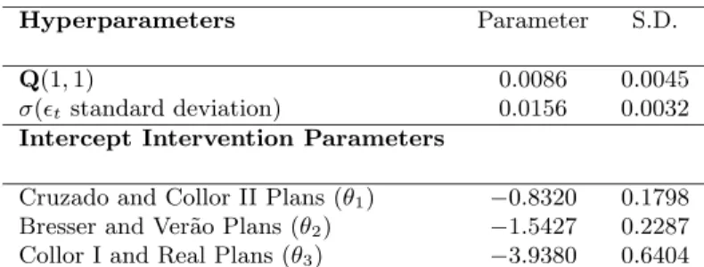
If we add this hypothesis to the already simplified 5 parameters TVP model, the number of parameters drops from 5 to 4, but the log likelihood drops from 111.43 to 107.87. The estimated values of the 5 parameters of the selected TVP model and those of the one-step ahead Theil-U7 can be found in table 2. The one-step ahead forecast and fitted values of the TVP model are presented in figure 3. The estimated NAIRU and its confidence interval are presented in section 6.
Table 2 TVP model
log likelihood = 111.43, Theil-U = 0.28
Hyperparameters Parameter S.D.
Q(1,1) 0.0086 0.0045
σ(ǫt standard deviation) 0.0156 0.0032
Intercept Intervention Parameters
Cruzado and Collor II Plans (θ1) −0.8320 0.1798
Bresser and Ver˜ao Plans (θ2) −1.5427 0.2287
Collor I and Real Plans (θ3) −3.9380 0.6404
5.2
The MSR model results and the stability of coefficients of the
price Phillips curve
The MSR model was initially estimated, in its more general version, with 15 parameters, if we exclude from the counting the parameters belonging to βt∗. It could not be rejected – at a significance level higher than 10% and using the likelihood ratio test – that all the parameters at the diagonal of matrix Q are equal to zero at state 2 and that these parameters (with the exception of the parameter that controls for the time variability of the intercept) are also equal to zero at state 1. With these restrictions, the MSR model has 8 parameters to be estimated through the numerical optimization routine.
7The one-step ahead Theil-U statistic is equal to
T
t=k+1
e2
t/ T
t=k+1
(∆πt−∆πt−1)2, where
et is the one-step ahead forecast error, k is the number of parameters of the model and T is
Table 1 presents the log likelihood for the simplified selected MSR model (with the above restrictions)as 121.09 and for the initial MSR model (without these re-strictions)as 121.26. Furthermore, as table 1 shows, if we impose the additional restriction of no time-varying intercept in state 1 (stable NAIRU), the number of parameters drops from 8 to 7 but the log likelihood drops from 121.09 to 113.14. Therefore, we cannot reject the stability of coefficients of the Brazilian price Phillips curve but, given this stability, we can reject a constant NAIRU.
Figure 3
TVP Model - One Step Ahead Forecast ofDp
-0.5 -0.4 -0.3 -0.2 -0.1 0 0.1 0.2
83.IV 86.IV 89.IV 92.IV 95.IV 98.IV quarters
Dp Forecast
01.IV
MSR Model - One Step Ahead Forecast ofDp
-0.50 -0.40 -0.30 -0.20 -0.10 0.00 0.10 0.20
83.IV 86.IV 89.IV 92.IV 95.IV 98.IV 01.IV quarters
Dp Forecast
TVP Model - FittingDp
-0.5 -0.4 -0.3 -0.2 -0.1 0 0.1 0.2
83.IV 86.IV 89.IV 92.IV 95.IV quarters
Dp Forecast
01.IV
MSR Model - Fitting Dp
-0.50 -0.40 -0.30 -0.20 -0.10 0.00 0.10 0.20
83.IV 86.IV 89.IV 92.IV 95.IV 98.IV quarters
Dp Forecast
01.IV
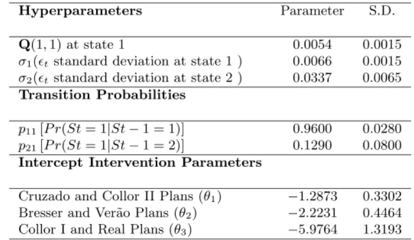
Table 3 MSR model
log likelihood = 121.09, Theil-U= 0.29
Hyperparameters Parameter S.D.
Q(1,1) at state 1 0.0054 0.0015
σ1(ǫtstandard deviation at state 1 ) 0.0066 0.0015
σ2(ǫtstandard deviation at state 2 ) 0.0337 0.0065
Transition Probabilities
p11[P r(St= 1|St−1 = 1)] 0.9600 0.0280
p21[P r(St= 1|St−1 = 2)] 0.1290 0.0800 Intercept Intervention Parameters
Cruzado and Collor II Plans (θ1) −1.2873 0.3302
Bresser and Ver˜ao Plans (θ2) −2.2231 0.4464
Collor I and Real Plans (θ3) −5.9764 1.3193
Table 4
Transition probability matrix (P)
St= 1 St= 2 St−1 = 1 0.960 0.040
St−1 = 2 0.129 0.871
Steady – State
probabilities 0.763 0.237
5.3
The comparison between the TVP and MSR models and some
additional statistical tests
Table 1 shows that the maximizing value of log likelihood for the selected MSR model is 121.09 and the same value for the selected TVP model is 111.43. The TVP model is more parsimonious than the MSR model, since it has 3 parameters less. It is also true that the TVP model (without ARCH residuals) is nested in the MSR model. Nevertheless, as it has been pointed out by Engel and Hamilton (1990), if the information matrix is singular in the region of the parameter space where the MSR model becomes the TVP model, then the standard regularity con-ditions needed to establish asymptotically valid hypothesis tests are not satisfied. Therefore, we cannot test, using the usual tests, which of the models better fits the data and the results, for both models are going to be presented.
Table 5
Additional hypothesis tests – MSR model
Ho∗:p
11=1−p22 Ho:Q1(1,1) =0
Wald test 179.15 12.58
Likelihood Ratio test 12.50 15.90
Log Likelihood (under Ho) 114.84 113.14 ∗Suggested by Engel and Hamilton (1990)
We did not detect significant serial correlation, in the MSR model, for either the standardized one-step ahead forecast error or the squares of the standardized one-step ahead forecast errors. Nevertheless, the same is not true for the TVP model. Tables 6 and 7 present these tests.
Table 6
Tests for serial correlation of standardized forecast errors
MRS MODEL TVP MODEL
Autocorrelation Partial Q-Statistic Probability Autocorrelation Partial Q-Statistic Probability
Correlation Correlation
1 0.210 0.210 3.5391 0.060 0.112 0.112 1.0071 0.316
2 −0.016 −0.063 3.5591 0.169 −0.218 −0.234 4.8715 0.088 3 −0.106 −0.094 4.4819 0.214 −0.185 −0.137 7.6755 0.053
4 −0.056 −0.014 4.7397 0.315 0.159 0.161 9.7834 0.044
5 −0.069 −0.063 5.1400 0.399 0.029 −0.086 9.8529 0.080 6 −0.190 −0.186 8.2412 0.221 −0.222 −0.203 14.078 0.029
7 −0.001 0.072 8.2414 0.312 −0.056 0.051 14.350 0.045
8 0.021 −0.017 8.2814 0.406 0.062 −0.049 14.694 0.065
9 −0.083 −0.141 8.9036 0.446 −0.053 −0.160 14.948 0.092 10 −0.064 −0.026 9.2744 0.506 −0.092 0.001 15.714 0.108
11 0.058 0.068 9.5794 0.569 0.023 0.005 15.763 0.150
12 −0.144 −0.266 11.525 0.485 −0.158 −0.342 18.102 0.113
13 −0.069 0.014 11.975 0.530 −0.029 0.053 18.183 0.151
14 −0.030 −0.011 12.064 0.601 0.015 −0.023 18.206 0.198
15 0.133 0.042 13.797 0.541 0.080 −0.156 18.839 0.221
16 0.011 −0.085 13.809 0.613 −0.108 −0.110 20.004 0.220 17 −0.026 0.023 13.878 0.676 −0.068 −0.008 20.472 0.251
18 0.294 0.271 22.807 0.198 0.287 0.155 28.992 0.048
19 0.135 −0.024 24.729 0.170 0.179 0.004 32.365 0.028
20 −0.038 −0.066 24.885 0.206 −0.114 −0.054 33.760 0.028 21 −0.180 −0.071 28.394 0.129 −0.172 −0.053 36.982 0.017 22 −0.105 −0.077 29.612 0.128 0.006 −0.137 36.987 0.024
23 −0.022 0.014 29.668 0.159 0.099 0.001 38.091 0.025
Table 7
Tests for serial correlation of squared standardized forecast errors
MRS MODEL TVP MODEL
Autocorrelation Partial Q-Statistic Probability Autocorrelation Partial Q-Statistic Probability
Correlation Correlation
1 0.203 0.203 3.2996 0.069 0.055 0.055 0.2379 0.626
2 0.016 −0.026 3.3215 0.190 0.218 0.215 4.0756 0.130
3 −0.071 −0.072 3.7315 0.292 0.166 0.153 6.3475 0.096
4 −0.070 −0.043 4.1399 0.387 0.016 −0.042 6.3685 0.173
5 0.057 0.084 4.4096 0.492 0.041 −0.029 6.5077 0.260
6 0.169 0.145 6.8681 0.333 0.287 0.289 13.582 0.035
7 −0.062 −0.144 7.2053 0.408 −0.019 −0.033 13.615 0.058
8 −0.074 −0.037 7.6944 0.464 0.146 0.024 15.498 0.050
9 −0.145 −0.098 9.5824 0.385 −0.076 −0.171 16.015 0.067
10 0.066 0.139 9.9768 0.443 −0.026 −0.028 16.078 0.097
11 0.067 −0.008 10.386 0.496 0.000 0.032 16.078 0.138
12 0.118 0.071 11.689 0.471 0.047 0.030 16.286 0.178
13 0.005 −0.009 11.692 0.553 −0.107 −0.125 17.377 0.183 14 −0.047 −0.014 11.906 0.614 −0.018 −0.104 17.409 0.235 15 −0.092 −0.050 12.728 0.623 −0.019 0.115 17.445 0.293
16 −0.005 −0.027 12.730 0.692 0.012 0.106 17.459 0.356
17 0.051 0.055 12.997 0.736 −0.005 −0.005 17.462 0.423
18 0.222 0.188 18.060 0.452 0.185 0.134 21.002 0.279
19 −0.021 −0.081 18.106 0.515 −0.105 −0.097 22.152 0.277
20 0.012 0.048 18.122 0.579 −0.041 −0.092 22.331 0.323
21 −0.042 −0.008 18.310 0.629 −0.051 −0.049 22.614 0.365 22 −0.074 −0.080 18.916 0.651 −0.107 −0.082 23.889 0.353
23 0.025 0.006 18.987 0.702 −0.033 −0.041 24.009 0.403
24 0.037 −0.038 19.144 0.744 −0.063 −0.154 24.463 0.435
6.
The Estimated NAIRU and the Response of
∆
π
to Cyclical
Unemployment
Figure 5
85.IV 89.IV 93.IV 97.IV 01.IV 2
4 6 8 10 12
TVP Model
quarters %
93.IV 95.IV 97.IV 99.IV 01.IV 2
4 6 8 10 12
TVP Model
quarters %
93.IV 95.IV 97.IV 99.IV 01.IV 2
4 6 8 10 12
MSR Model
quarters %
85.IV 89.IV 93.IV 97.IV 01.IV 2
4 6 8 10 12
MSR Model
quarters %
Unemployment Nairu - - - Confidence Intervals
Error Bands for Nairu
Smoothed Estimations – 95% confidence Intervals (1,000 simulations at each date)
After the Real Plan, there is growing evidence of the presence of seasonality in the unemployment data. Therefore, we also have estimated both previously selected models, with seasonally adjusted unemployment data8. The estimated NAIRU and its confidence intervals for both models, with seasonally adjusted unemployment data, are presented in figure 6.
The cyclical unemployment is defined as the difference, at each datet, between the observed rate of unemployment and the estimated NAIRU. If we consider as given the cyclical unemployment then, from equation (1), we get:
8The unemployment rate was seasonally adjusted using the x12-arima software. The presence
∆πt=µt+
3
s=1
βsCt−s+
2
s=1
γs∆πt−s+ǫt (1”)
whereCt=ut−ut = cyclical unemployment.
Figure 6
...
85.IV 89.IV 93.IV 97.IV 01.IV
2 4 6 8 10 12 MSR Model quarters %
93.IV 95.IV 97.IV 99.IV 01.IV
2 4 6 8 10 12 MSR Model quarters %
85.IV 89.IV 93.IV 97.IV 01.IV
2 4 6 8 10 12 TVP Model quarters %
93.IV 95.IV 97.IV 99.IV 01.IV
2 4 6 8 10 12 TVP Model quarters %
Seasonally adjusted Unemployment Nairu - - - Confidence Intervals
Error Bands for Nairu – with seasonally adjusted unemployment data
Smoothed Estimations – 95% confidence Intervals (1,000 simulations at each date)
The response of ∆πt (the first difference of inflation) to a permanent +0.5%
cyclical unemployment, which has started at period t-h, can be computed through the following recursions:
θ(1) = 1 andθ(n) =
n i=2
min{i−1,2}
k=1
[γk.θ(i−k)]
;n= 1,2, . . .
R(0) = 0 andR(h) = 0.5∗12∗
h
i=1
i
k=1
min{k−1,3}
m=0
βm θ(k−m), h= 1,2, ....
R(h) is the annualized percent response of ∆π to a 0.5% cyclical unemployment that has been persistent for the lasth quarters. Given the distributions of the pa-rameters of equation (1′′), we can construct error bands for R(h) through Monte Carlo simulations. Figure 7 presents the cyclical unemployment,R(h) and its error bands for the TVP and MSR models with nonseasonally adjusted unemployment. Figure 8 presents the same results for the TVP and MSR models when both are estimated using seasonally adjusted unemployment.
Figure 7
85.IV 89.IV 93.IV 97.IV 01.IV -6
-4 -2 0 2
Cyclical Unemployment - MSR
quarters
%
85.IV 89.IV 93.IV 97.IV 01.IV -6
-4 -2 0 2
Cyclical Unemployment - TVP
quarters
%
1 3 5 7 9 11
-25 -20 -15 -10 -5
0
Response to +0.5% Cyclical Unemployment - MSR
quarters
Dp (%)
1 3 5 7 9 11
-25 -20 -15 -10 -5
0
Response to +0.5% Cyclical Unemployment - TVP
quarters
Dp (%)
Estimated Value --- 95% Confidence Intervals (1000 simulations)
Figure 8
85.IV 89.IV 93.IV 97.IV 01.IV
-6
-4 -2 0 2
Cyclical Unemployment - TVP
quarters
%
1 3 5 7 9 11 -25
-20 -15 -10 -5 0
Response to +0.5% Cyclical Unemployment - TVP
quarters
Dp
(%)
85.IV 89.IV 93.IV 97.IV 01.IV -6
-4 -2 0 2
Cyclical Unemployment - MSR
quarters
%
1 3 5 7 9 11 -25
-20 -15 -10 -5 0
Response to +0.5% Cyclical Unemployment - MSR
quarters
Dp
(%)
Estimated Value --- 95% Confidence Intervals (1000 simulations)
Cyclical Unemployment and the Response of the Change in Annual
Inflation Rate (Dp) to Cyclical Unemployment (with seasonally adjusted unemployment data)
The main conclusions are as follows: There is a statistically significant rela-tionship between cyclical unemployment and the change in inflation rate; if the TVP model is considered, a permanent 0.5% cyclical unemployment, after 3 quar-ters, reduces by 7.5% the annualized monthly inflation rate; if the MSR model is considered a permanent 0.5% cyclical unemployment, after 1 quarter, reduces by 5% the annualized monthly inflation rate.
7.
Conclusions
significantly different from the observed rate of unemployment across time? The first question can be easily answered by observing the response of inflation to cyclical unemployment, presented in section 5. There is a significant and neg-ative response of inflation to an increase in cyclical unemployment. Nevertheless the effect is not measured with high precision if we consider model uncertainty. The response of annual inflation to 0.5% cyclical unemployment that is persistent for 3 quarters belongs, with a 95% degree of confidence, to the (−11%,−7.5%) interval for the TVP model and to the (−6%,−4%) interval for the MSR model. The two models do not allow for time-varying coefficients for lag unemployment and lag inflation. Therefore, it cannot be rejected that the deviations of the rate of unemployment from the NAIRU can have a significant effect, with correct sign, on the rate of inflation. Nevertheless, it is also true that the above estimates of the effect are not very precise. If we consider the uncertainty with respect to what the right model is, then any value between −11% and−4% cannot be rejected.
The answer to the second question depends on the degree of precision with which the NAIRU is estimated. Observing figures 5 and 6 we can conclude that the estimates of the NAIRU, considering both models, are very imprecise and that from the second quarter of 1995 the estimated value of the NAIRU is contained within its error bands and therefore it cannot be rejected that the observed rate of unemployment was equal to the NAIRU.
References
Akerlof, G. A., Dickens, W. T., & Perry, G. L. (1996). The macroeconomics of low inflation. Brookings Papers on Economic Activity, (1):1–76.
Akerlof, G. A., Dickens, W. T., & Perry, G. L. (2000). Near-rational wage and price setting and the optimal rates of inflation and unemployment. Brookings Papers on Economic Activity, (1). forthcoming.
Albert, J. & Chib, S. (1993). Bayes inference via gibbs sampling of autoregressive time series subject to markov mean and variance shifts. Journal of Business and Economic Statistics, 11.
Blanchard, O. & Katz, L. F. (1997). What we know and do not know about the natural rate of unemployment. The Journal of Economic Perspectives, 11(1).
Cogley, T. & Sargent, T. J. (2001). Evolving post-world war II U. S. inflation dynamics. mimeo.
Corseuil, C. H., Gonzaga, G., & Issler, J. V. (1996). Desemprego regional no Brasil: Uma abordagem emp´ırica. S´erie semin´arios da Diretoria de Pesquisa do Ipea, n0 09/96.
Engel, C. & Hamilton, J. D. (1990). Long swings in the dollar: Are they in the data and do markets know it? The American Economic Review, 80:689–713.
Friedman, M. (1968). The role of monetary policy. American Economic Review, 68(1):1–17.
Gordon, R. J. (1982). Inflation, flexible exchange rates, and the natural rate of unemployment. In Baily, M. N., editor,Workers, Jobs and Inflation. Brookings.
Gordon, R. J. (1997). The time-varying NAIRU and its implications for economic policy. Journal of Economic Perspective, 11(1):11–32.
Gordon, R. J. (1998). Foundations of the goldilocks economy: Supply shocks and the Time-Varying NAIRU. Brooking Papers on Economic Activity, 2:297–333.
Hamilton, J. D. (1989). A new approach to the economic analysis of nonstationary time series and the business cycle. Econometrica, 57(2):357–384.
Harrison, P. J. & Stevens, C. F. (1976). Bayesian forecasting.Journal of the Royal Statistic Society, 38:205–247. Series B 38.
Harvey, A. C. (1989). Forecasting Structural Time Series Models and the Kalman Filter. Cambridge University Press, Cambridge.
Harvey, A. C., Ruiz, E., & Sentana, E. (1992). Unobserved component time series models with ARCH disturbances. Journal of Econometrics, 52:129–157.
Katz, L. F. & Krueger, A. B. (1999). The high-pressure U.S. labor market of the 1990’s. Brookings Papers on Economic Activity, 1:1–87.
Kim, C. & Nelson, R. C. (1998). The time-varying-parameter model for modeling changing conditional variance: The case of the lucas hypothesis. Journal of Business and Economic Statistics, 7(4):433–440.
Kim, C. & Nelson, R. C. (1999). State Space Models with Regime Switching. The MIT Press, London, England.
Kim, C.-J. (1994). Dynamic linear models with Markov-switching. Journal of Econometrics, 60:1–22.
King, R. G., Stock, J. H., & Watson, M. (1995). Temporal instability of the unem-ployment – inflation relationship. Economic Perspectives, pages 2–12. Federal Reserve Bank of Chicago.
King, R. G. & Watson, M. W. (1994). The post-war U.S. Phillips curve: A revisionist econometric history. Carnegie-Rochester Conference Series on Public Policy, 41:157–219.
Lundbergh, S., Ter¨asvirta, T., & Van Dijk, D. (2002). Time-varying smooth transition autoregressive models. Journal of Business and Economic Statistics.
Portugal, M. S., Madalozzo, R. C., & Hilllbrecht, R. O. (1999). Inflation, unem-ployment and monetary policy in Brazil. mimeo.
Rogerson, R. (1997). Theory ahead of language in the economics of unemployment.
Sargent, T. J. (1971). A note on the accelerationist controversy. Journal of Money Credit and Banking, 8(3):721–725.
Shephard, N. (1994). Partial non-gaussian state space. Biometrika, 81:115–131.
Sims, C. A. (1999). Drift and breakes in monetary policy. Discussion paper, Princeton University, http://www.princeton.edu/ Sims/.
Sims, C. A. & Zha, T. (2002). Macroeconomic switching. Discussion paper, Princeton University, http://www.princeton.edu/ Sims/.
Smith, A. F. M. & Makov, U. E. (1980). Bayesian detection and estimation of jumps in linear systems. In Jacobs, O. L. R., Davis, M. H. A., Dempster, M. A., & Harris, C. J. & Parks, P. C., editors,Analysis and Optimization of Stochastic Systems, pages 333–345. Academic Press, New York.
Staiger, D., Stock, J. H., & Watson, M. W. (1997). The NAIRU, unemployment and monetary policy. The Journal of Economic Perspectives, 11(1).
Staiger, D., Stock, J. H., & Watson, M. W. (2001). Prices,wages and the U.S. NAIRU in the 1990’s. mimeo.
Taylor, J. B. (2000). Low inflation, pass-through, and the pricing power of firms.
European Economic Review, 44:1389–1408.
Ter¨asvirta, T. (1994). Specification, estimation, and evaluation of smooth tran-sition autoregressive models. Journal of the American Statistical Association, 89:208–218.
Appendix
Let,
ψt−1 = [yt−1, yt−2, ...., y1] , information available up to time t-1;
βt∗|(ti,j−1)=E(βt∗ψt−1, St=j, St−1 =i) ;
(i,j)
t|t−1 =E[(β∗t −βt/t∗ −1)(βt∗−β∗t/t−1)′/ψt−1, St=j, St−1 =i] ;
βt∗−(i1)|t−1 =E(βt∗−1/ψt−1, St−1=i);
(i)
t−1|t−1 =E[(βt∗−1−βt∗−1/t−1)(β∗t−1−βt∗−1/t−1)′/ψt−1, St−1 =i];
Pr [St=j, St−1 =i] =piJ;
P= [pij] = matrix of transition probabilities;
Pr [St=i|ψt] = probability of state i , at period t, given information up to
timet.
The objective of Kim’s nonlinear filter is to obtain estimates of the unob-served state vector (β∗
t) and its associated mean squared error matrix (Σt), and
of the marginal probability of the latent Markov state variable St , at each date t. The estimates are based on information available up to time t. That is, at each date t, given βt∗−(i1)|t−1, (i)
t−1|t−1, Pr[St−1 =i|ψt−1], yt, Qj, σj, (for i= 1,2 and j = 1,2), θτ(τ = 1,2 and 3) and the matrix of transition probabilities (P) the Kim’s filter allows us to obtain approximate estimations of βt∗|(ti), Σ(ti|t), and Pr[St = j|ψt](j = 1,2). To start the filter we need the initial values of β0∗|(0i),
Σ(0i|)0 and Pr[S0 = i/ψ0](i = 1,2). We set β0∗|(0i) = 0 , Σ0(i|)0 = Ix100.000 and Pr[S0 =i/ψ0] (i= 1,2) equal to the ergodic distribution of the Markov chain (the steady-state marginal distribution of the states). What we have called Kim filter is actually a combination of the Kalman filter, Hamilton filter and a collapsing procedure. We describe the Kim filter below9.
9A detailed discussion of the Kim’s filter can be found in Kim (1994) and Kim and Nelson
Part I of Kim Filter - The Kalman Filter
Given β∗t−(i1)|t−1, (i)
t−1|t−1, yt, Qi , σi,( for i = 1,2) and θτ(τ = 1,2,3), the Kalman Filter gives β∗t|(ti,j), (i,j)
t|t , the conditional one-step prediction
er-ror (ηt(|i,jt−)1), and the conditional variance of the one-step prediction error, ft(|i,jt−)1
( for i= 1,2 and j = 1,2). The algorithm estimates 2 (number of different pos-sible regimes) state vectors for each pospos-sible value of St−1. Therefore, at each date t, the algorithm estimates 4 state vectors. The Kalman filter recursions are presented below:
Prediction equations:
βt∗|(ti,j−1)=βt∗−(i1)|t−1
(i,j)
t|t−1 = (i)
t−1|t−1+Qj Updating equations:
η(t|i,jt−)1 =yt−βt∗|(ti,j−1)xt
ft(|i,jt−)1 =xt(ti,j|t−)1x
′
t+σj2
βt∗|(ti,j)=βt∗|t(−i,j1)+(i,j)
t|t−1x ′
t f
(i,j)
t|t−1 −1
η(t|i,jt−)1
(i,j)
t|t = (I−
(i,j)
t|t−1x ′
t f
(i,j)
t|t−1 −1
xt)(ti,j|t−)1
Part II of Kim Filter - The Hamilton Filter
Given Pr [St−1 =i|ψt−1],P,ηt(|i,jt−)1,ft(|i,jt−)1, the Hamilton Filter obtains Pr[St−1 = i, St = j|ψt] and Pr[St = i|ǫt]. The Hamilton Filter is presented
below:
Pr [St=j, St−1 =i|ψt−1] = Pr [St=j, St−1 =i] Pr [St−1 =i|ψt−1],(i, j= 1,2)
Pr [St−1 =i, S1=j|ψt] =
f(yt|St−1 =i, St=j, ψt−1) Pr [St−1 =i, St=j|ψt−1]
Pr [St=j|ψt] =
2
i=1
Pr [St−1 =i, St=j|ψt]
Where,
f(yt|St−1 =i, St=j, ψt−1) = (2π)−
1 2 f
(i,j)
t|t−1 1 2 exp −1 2η (i,j)
t|t−1, f (i,j)−1
t|t−1 η (i,j)
t|t−1
(i, j= 1,2)
and
f(yt|ψt−1) = 2 j=1 2 i=1
f(yt|St=j, St−1=i, ψt−1) Pr [St=j, St−1 =i|ψt−1]
Part III of Kim Filter - The Collapsing
Given β∗t|(ti,j), (i,j)
t|t (both estimated by the Kalman filter) , Pr
St−1 = i ,
St=j|ψt, Pr [St=i|ψt] (both estimated by the Hamilton filter) andP, the filter
collapsesβ∗t|(ti,j)intoβt∗|(tj) and(i,j)
t|t into
(j)
t|t. The collapsing is of crucial
impor-tance because without it the number of filter evaluations is multiplied by 2, at each date t, and it is computationally unfeasible to estimate the model. The collaps-ing is an approximation based on the work of Harrison and Stevens (1976). The approximation consists of a weighted average of the updating procedures by the probabilities of the Markov state, in which the mixture of 4 Gaussian densities is collapsed, after each observation, into a mixture of 2 densities. It is done as follows:
Collapsing equations:
βt∗|(tj)= 2
i=1
Pr [St−1 =i, St=j|ψt]βt∗|(ti,j)
Pr [St=j|ψt]
(j)
t|t =
2
i=1
Pr[St−1=i,St=j|ψt]
(i,j)
t|t +
βt∗|(ti)−β∗t|(ti,j)βt∗|(ti)−β∗t|(ti,j)
′
The Likelihood
The likelihood is given by : L= T
t=1
f(yt/ψt−1)
The Recursive Estimates
βt∗|t= 2
j=1
βt∗|(tj)Pr [St=j|ψt]
Σt|t= 2
j=1
Σ(t|jt)Pr [St=j|ψt]
Therefore, given p11 , p22 , θτ(τ = 1,2,3) , σi (the measurement equation
residual’s standard deviation at state i, i = 1,2), and the 4 parameter at the diagonal o matrix Qi at each state, we can use the Kim’s filter to estimate β∗t|t,
Σt|t, Pr [St=j|ψt] and calculate the value of the likelihood of the MSR model. The
Kim filter obtains the nonlinear mapping from the hyperparameters (σiandQi;i=