Pesqui. Oper. vol.27 número2

TIME TO FAILURE ASSESSMENT OF PRODUCTS AT SERVICE CONDITIONS FROM ACCELERATED LIFETIME TESTS WITH

STRESS-DEPENDENT SPREAD IN LIFE

Enrique López Droguett *

Department of Production Engineering Federal University of Pernambuco (UFPE) Recife – PE, Brazil

[email protected]

Ali Mosleh

Reliability Engineering Program University of Maryland

College Park – MD, USA

* Corresponding author / autor para quem as correspondências devem ser encaminhadas

Recebido em 11/2005; aceito em 03/2007 Received November 2005; accepted March 2007

Abstract

In accelerated lifetime testing (ALT) the assumption of stress-independent spread in life is commonly used and accepted because the resulting models are typically easier to use and data or past experience suggest that such a constrain is sometimes valid. However in many situations and with a variety of products the spread in life does depend on stress, i.e., the failure mechanism is not the same for all stress levels. In this paper the assessment of product time to failure at service conditions from ALT with stress-dependent spread is addressed by formulating a Bayesian framework where the time to failure follows a Weibull distribution, scale parameter dependency on stress is given by the Power Law, and two cases for the dependency between shape parameter and stress are discussed: linear relationship and, in order to allow a comparative analysis, stress-independent shape parameter. A previously published dataset is used to illustrate the procedure.

Keywords: accelerated lifetime testing; Weibull distribution; Bayes’ theorem; reliability.

Resumo

Em testes acelerados de vida (ALT) a suposição de que a dispersão do tempo de falha é independente do stress é freqüentemente empregada e aceita pois os modelos resultantes são tipicamente mais fáceis de utilizar e dados ou experiência adquirida sugerem que tal simplificação é algumas vezes válida. Entretanto, em muitas situações e para uma variedade de produtos, a dispersão do tempo de falha depende do stress, i.e., o mecanismo de falha não é o mesmo em todos os níveis de stress. Neste artigo, a estimação do tempo de falha do produto nas condições de serviço a partir de ALT com dispersão dependente do stress é discutida através da formulação de um modelo Bayesiano onde o tempo de falha segue uma distribuição de Weibull e o parâmetro de forma é dependente do stress via uma relação linear. Um conjunto de dados anteriormente publicado é utilizado para ilustrar o procedimento.

Palavras-chave: testes acelerados de vida; distribuição de Weibull; teorema de Bayes;

1. Introduction

In many areas, difficulties in obtaining significant failure data for reliable products under service (normal) operational conditions, the speed of advance in technology that keeps pushing the necessity of gathering data in short periods of time before the product under development becomes obsolete, and the requirements to meet deadlines and cost constrains lead reliability engineers, statisticians and other specialist to consider accelerated life testing as the only available technique in order to overcome these obstacles.

In an accelerated life test products are subjected to higher stress conditions than those for which they are designed to operate (service conditions) forcing the products to fail more quickly than it would have under service conditions. As a result, ALT reduces the test time and still provides valuable information for the manufacturer to understand the failure process (failure modes and related failure mechanisms and causes) impacting the reliability characteristics of products.

In designing an accelerated life test special attention should be given to how stresses and stress levels are chosen. In fact, they should be chosen so that they accelerate failure modes under investigation but do not introduce failure modes that would never occur under service conditions. Furthermore, it is considered that the time to failure T of a product being tested is a random variable distributed according to a probability distribution f T( | )θ that depends on a unknown set of parameters θ. Furthermore, it is assumed that all or some of the parameters θ (in general the scale parameter for the Weibull distribution or mean log life for the Lognormal distribution) are related to the stress s under which the test is carried out by a specified function of the form θ ψ ω= ( , )s , where the set of parameters ω determine the relationship between θ and s. The function ψ ω( , )s is known as Acceleration or Time Transformation. It is important to note that in the case of more than one parameter being dependent on the stress s, each one can be related to s by a different relationship ψ .

The goal of accelerated life testing is to make inferences about the failure times of products operating at normal stress conditions based on observed failure data under accelerated stress conditions. To do so, however, it is imperative to estimate the set of parameters θ and ω. Thus, assumptions on the distribution of the times to failure and on the functional relationship between the parameters of the failure distribution and the applied stress, ψ , must be made. A common assumption is that, for all stress levels, the failure times are governed by the same parametric family of probability distributions such as Lognormal or Weibull distributions, and the time transformation ψ is assumed to follow a parametric model such as the Arrhenius Law, Eyring Law or the Power Law.

belt webbings where lifetimes were predicted by performing accelerated life tests which were designed using temperature, UV irradiance and abrasion as stress factors. The ALT was carried out for each stress factor at a time and the validity of the stress-independent assumption was confirmed by using the Bonferroni’s simultaneous confidence interval (Nelson, 1982). ALT data is also a valuable source of evidence during the development stages of a new product. In this context, Groen & Droguett (2005) and Groen et al. (2004) have developed a Bayesian reliability assessment methodology for products under development that take into account different sources of evidence such as field data and prototype accelerated lifetime test data.

In many situations however the stress-independent assumption is no longer valid. For instance, Nelson (1984) studies the fitting of fatigue curves to experimental data where the standard deviation is a function of stress. Also, Barlow et al. (1988) considers the case of the stress-rupture life of Kevlar/Epoxy strands and show that such accelerated life testing data are Weibull distributed with a stress-dependent shape parameter. However no further insights in the accelerated life testing modeling and lifetime prediction at service conditions are provided.

Available methodologies and applications concerning accelerated life testing have been documented by Nelson (1982), Kececioglu (1993), Tobias & Trindade (1995), Bagdonavicius & Nikulin (2002), to name just a few. These studies present a significant understanding on the modeling and analysis of accelerated tests. However, the issue of time to failure assessment at service conditions given a scenario of stress-dependent spread in life (e.g., standard deviation of log life in a Lognormal distribution or the shape parameter in a Weibull distribution) has not yet been fully addressed.

The purpose of this paper is to address the issue of ALT with stress-dependent spread in life, and the application of the stress is independent of time, i.e., the stress level applied to a sample of units does not vary with time. This is presented with a formulation of a Bayesian model in which the time to failure distribution is assumed to follow a Weibull distribution, the scale parameter follows the Power Law, and the shape parameter is considered to be dependent on stress. The proposed model is validated using data obtained via Monte Carlo sampling method. The case where the shape parameter is assumed to be independent on stress is also presented and discussed under a Bayesian framework. Both models (stress-independent and stress-dependent shape parameter) are used to fit previously published real censored data where clearly the shape parameter is strongly dependent on stress. The results from both models are compared and the fit checked.

The paper is organized as follows. The next section discusses the models proposed in this work for both cases comprehending constant and stress-dependent shape parameter. Then, the proposed Power-Weibull model with linear stress-dependent shape parameter is validated via a Monte Carlo generated data set. Section 4 presents an example of application in the context of the lifetimes of Kevlar/Epoxy Spherical Pressure Vessels. Section 5 provides some insights from the comparison between the Power-Weibull with constant and linear shape parameter models. Then some concluding remarks are provided.

2. Model Development

Let us assume that at any stress level s the time to failure T is distributed according to a Weibull distribution with the following probability density function (Weibull, 1951)

( ) ( ) 1

( ) ( ) ( ) ( ; ) ( ) s t s s s s t

f t s e

s β β α β β α   − _{− }   = (1)

and reliability function given by (Weibull, 1951)

( ) ( ) ( ; ) s t s R t s e

β α

 

−_ _

= (2)

where α( )s is a scale parameter and β( )s is a shape parameter, both considered to be dependent on stress, s.

Sometimes, however, it is useful (from a computational perspective) to analyze Weibull data under the Smallest Extreme Value Distribution and such procedure is applied in this paper for the cases where the dependency on stress is analyzed. Indeed, if the time to failure T is Weibull distributed, then the natural log of time to failure Y=ln( )T has an extreme value distribution with the following probability density function (Gumbel, 1958)

( ) ( ) ( ) ( ) 1 ( ; ) ( ) y s s y s e s

f y s e e

s λ ξ λ ξ ξ −       −    _{ −}   = (3)

and reliability function (Gumbel, 1958)

( ) ( ) ( ; ) y s s e

R y s e

λ ξ −       − = (4)

where ( ) 1/ ( )ξ s = β s is a scale Parameter and ( )λ s =ln[ ( )]α s is a location parameter.

2.1 The Power-Weibull Model: General Modeling

This section initially presents a general modeling in which we do not assume any particular functional relationship between the scale parameter and stress or the shape parameter and stress, but it is assumed that at any stress level s_j the failure times or the censored times are distributed according to the same parametric probability distribution. The general model deduction is performed using the natural log of life Y≡ln( )T , which is Extreme Value distributed with scale parameter ( ) 1/ ( )ξ s = β s and location parameter ( )λ s =ln[ ( )]α s .

Assume that the available evidence at each stress level s_j is composed by a series of u

failure times t₁,K,t_i, i∈u, or equivalently for log times

1, , i

y K y, i∈u, and c singly or multiply censored times t₁,K,t_i, i∈c, which correspond to the log times

1, , i y K y, i∈c. The likelihood for a failure at y_i, i∈u is the probability density function given by equation (3) evaluated at y_i, and at s_j as one has to take into account the effect of stress into the

distribution parameters ( )λ s and ( )ξ s . Then,

( , | ( ), ( )) ( | ( ), ( ))

i i j j j i j j

or, ( ) ( ) ( ) ( ) 1 ( , | ( ), ( )) ( )

yi sj

i j

s j j

y s

s e

i i j j j

j

L y s s s e e

s λ ξ λ ξ ξ λ ξ  −         −     _{ −}   = (6)

The likelihood for a censored observation at y_i, i∈c and stress level s_j is the survival probability for the Extreme Value distribution, namely,

'

( , | ( ), ( )) ( , | ( ), ( ))

i i j j j i i j j

L y s ξ s λ s =R y s ξ s λ s (7)

Taking equation (4) into equation (7) results in the likelihood function for each censored time:

( )

( ) '

( , | ( ), ( ))

yi sj s j e

i i j j j

L y s s s e

λ ξ ξ λ  −        − = (8)

The total likelihood for the n=u+c specimens under test at stress level s_j is

( ) ( ) ( ) ( ) ( ) ( ) 1 ( , | ( ), ( )) ( )

yi sj yi sj

i j

sj sj

j

y s

s _{e e}

j i j j j

i u j i c

L y s s s e e e

s λ λ ξ ξ λ ξ ξ λ ξ  −   −               −     _{ − −}   ∈ ∈         = _{   }      

∏

∏

As we have a total of m stress level, the final form for the likelihood function is given by the following expression: ( ) ( ) ( ) ( ) ( ) ( ) 1 1 ( , | ( ), ( )) ( )

y_ij s_j y_ij s_j

ij j

sj sj

j

y s

m

s _{e e}

i j j j

j i u j i c

L y s s s e e e

s λ λ ξ ξ λ ξ ξ λ ξ  −   −               −     _{ − −}   = ∈ ∈       _{   } =  _{   }  _{   }  

∏ ∏

∏

Let D represent the total available evidence. If π ξ0( ( ), ( ))s λ s is the prior distribution for the parameters ( )λ s and ( )ξ s , the posterior distribution of the model parameters is as follows:

( ) ( ) ( ) ( ) ( ) ( ) ( ) ( ) 1 ( ) ( ) 1 ( ( ), ( )) ( ) ( ( ), ( )| ) 1 ( )

yij sj yij sj ij j

sj sj

j

yij sj ij j

s j j

y s

m

s e e

o j

j i u i c

y s

s e

j

e e e s s

s

s s D

e e s λ λ ξ ξ λ ξ λ ξ λ ξ

π ξ λ

ξ

π ξ λ

ξ  −   −               −     −     _{ − −}   = ∈ ∈  −     _{ −}         _{    ⋅}  _{   }  _{   }   =

∏ ∏

∏

yij sj s j m

e

o

j i u i c

e s s d d

λ ξ

ξ λ π ξ λ ξ λ

 −         ₋  = ∈ ∈       _{    ⋅} _{⋅ ⋅}  _{   }  _{   }  

∏ ∏

∏

∫ ∫

2.2 Power-Weibull Model with Constant Shape Parameter

section 4 (Barlow et al., 1988). Then, one can write α_{( )s} =_eγ0_/sγ1 _where 0

γ and γ₁ are parameters to be estimated from data. In the case of log life Y≡ln( )T , the location parameter λ( )s =ln[ ( )]α s assumes a linear function in Log (base e) stress given by

0 1

( )s ln( )s

λ = − ⋅γ γ .

Under the assumption of stress-independent shape parameter, it is possible to write ( )s

β =β. This results in the following scale parameter of a Extreme Value distribution: 1/

ξ= β , which is to be estimated from accelerated life testing data.

Inserting the location and scale parameters ( )λ s and ξ in equation (10), the total likelihood function for the Power-Weibull model with constant shape parameter is given by

[0 1ln( )] [0 1ln( )] 0 1

[ ln( )]

1 1 ( , | , ( ))

yij s yij s

ij

y s

m

e e

i j j

j i u i c

L y s s e e e

γ γ γ γ

ξ ξ γ γ ξ ξ λ ξ − − − −                 − −    _{ − −}   = ∈ ∈       _{   } = _{ }      _{   }  

∏ ∏

∏

Using equation (12) and a generic prior distribution, the posterior probability distribution of the parameters θ ={ ,ξ γ γ₀, }₁ has the following form:

[0 1ln( )] [0 1ln( )] 0 1

[ ln( )]

1 0 1

1 1

( | ) ( , , )

yij s yij s

ij

y s

m

e e

o

j i u i c

D k e e e

γ γ γ γ

ξ ξ

γ γ ξ

π θ π ξ γ γ

ξ − − − −                 − −    _{ − −}   = ∈ ∈       _{   } = ⋅ _{ }⋅      _{   }  

∏ ∏

∏

where k₁ is a normalizing constant.

2.3 Power-Weibull Model with Stress-Dependent Shape Parameter

Several functional forms for the shape parameter have been proposed. In general, one can consider β( )s =g s( ;δ δ₀, ₁,K) where g( )g is a specified function and

0, 1,

δ δ K are parameters to be determined from the accelerated life testing data. A simple relationship is the linear model, β( )s =δ₀+ ⋅δ₁ s, or in alternate form β( )s =δ₀+ ⋅δ₁ ln( )s . Another

possible formulation is to consider a quadratic term in stress β( )s =δ0+ ⋅ + ⋅δ1 s δ2 s2 which has the property to describe a shape parameter the can, for example, initially increase with stress and after a certain stress level, it decreases as further stresses are applied.

From this, the equivalent extreme value distribution has parameters ξ( ) 1/[s = δ₀− ⋅δ₁ ln( )]s and λ( )s = − ⋅γ0 γ1 ln( )s . We will refer to this model as Power-Weibull-Linear Model. Therefore, the likelihood for the Power-Weibull model with non constant shape parameter is:

[0 1ln( )] [0 1ln( )] 0 1

1 1

1 [0 1ln( )] [0 1ln( )] 0 1

[ ln( )]

[ ln( )]

0 1

1

( , | ( ), ( )) [ ln( )]

yij s yij s

ij

s s

y s

m

s e e

i j j j

j i u i c

L y s s s s e e e

γ γ γ γ

δ δ δ δ

γ γ δ δ

ξ λ δ δ

 − −   − −      − −     −  −   −  − −      ₋  _{− −}   = ∈ ∈       _{   } =  _ − _{  }  _{   }  

∏ ∏

∏

The posterior probability distribution for the parameters θ={ , ,γ γ δ δ_{0 1 0}, }₁ is then given by

[0 1ln( )] [0 1ln( )] 0 1

1 1

1 [0 1ln( )] [0 1ln( )] 0 1

[ ln( )]

[ ln( )]

2 0 1 0 1

1 1

( | ) ( , , , )

yij s yij s

ij

s s

y s

m

s e e

o

j i u i c

D k e e e

γ γ γ γ

δ δ δ δ

γ γ δ δ

π θ π γ γ δ δ

ξ  − −   − −      − −     −  −   −  − −      ₋  _{− −}   = ∈ ∈       _{   } = ⋅ _{    }⋅  _{   }  

∏ ∏

∏

where k₂ is a constant of normalization.

3. Model Validation

This section presents the validation of the proposed model using a simulated data set via Monte Carlo (Fishman, 2000). The life percentiles at a given stress will be calculated and checked against the corresponding ones from the simulated data.

From the reliability function for a Extreme Value distribution given by equation (4), one can get the cumulative probability distribution in which both the location and the scale parameters are function of the stress as

( ) ( )

( ; ) 1

y s s e

F y s e

λ ξ−       −

= − (16)

From equation (16) it is easy to show that log life p-th percentiles at any stress are given by λ_p( )s =λ( ) ln[ ln(1s + − −p)]⋅ξ( )s . The shape parameter is β( )s =δ0− ⋅δ1 ln( )s and

consequently the Extreme Value distribution scale parameter is ξ( ) 1/[s = δ₀− ⋅δ₁ ln( )]s . The Weibull scale parameter α( )s is assumed to follow the Power Law and, as before, the Extreme Value location parameter is λ( )s = − ⋅γ₀ γ₁ ln( )s . The corresponding life p-th

percentiles can be obtained from y_p( )s as tp( )s e ( ) ln[ ln(1s p)] ( )s ( ) [ ln(1s p)]1/ ( )s

λ + − − ⋅ξ _α β

= = ⋅ − − .

6 27.704

s = MPa (Ln[s₆] = 3.32 MPa, 40% stress level). Further, assume that the hypothetic goal of the experiment is to estimate the life percentile at 40% stress level.

Note that the 40% stress level is not used to generate the posterior life percentiles, thus providing a way to check the extrapolation to lower stress levels. In Figure 1 and Figure 2 are presented the generated time percentiles for 90% and 40% stress levels respectively. In order to estimate the life percentiles at 40% or lower stress levels, the simulated data set was modeled by the Power-Weibull model with stress-dependent shape parameter (equation (15)). It is used a constant prior distribution for the parameters γ γ δ δ0, 1, 0, 1.

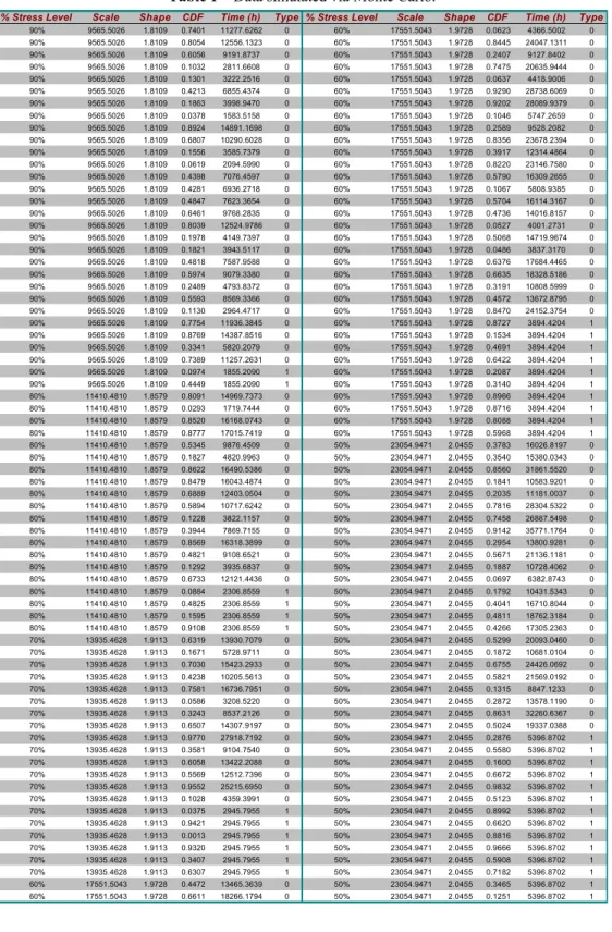
The data set generated via Monte Carlo is shown in Table 1 where type 0 means failure time and type 1 means censored time. Note that the number of data points is not equal for all the stress levels. Although the actual numbers of data points were randomly generated, units were allocated per stress level following a typical strategy used in accelerated testing (Nelson, 1990), i.e., one tends to preferably allocate more units at stress levels that are closer to the targeted use conditions. Also note that, as one would expect in a real situation, the higher is the applied stress, the lower is the number of censored units. In Table 2 are shown the parameters estimate γ γ δ δˆ₀,ˆ₁,ˆ₀,ˆ₁ at the likelihood mode. Note that these values are not obtained via application of a maximum likelihood method, but instead they are the parameters values corresponding to the mode of the joint likelihood function of equation (15).

Figure 1 – Percentiles for 90% stress level. Figure 2 – Percentiles for 40% stress level.

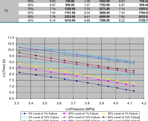
Through the application of the Bayesian inference technique represented by equation (15) to the simulated data, the time to observe 1% and 50% failure fractions at different stress levels were calculated from π γ γ δ δ( 0, 1, 0, 1|D), posterior probability density function of the parameters, and are presented in Figure 3 and Figure 4, respectively. Note that in order to appropriately measure the uncertainty in the estimated times for specific failure fractions, the probability intervals are also provided ranging from 1% to 99% for a given failure level.

In order to check the results obtained from the Power-Weibull-Linear model one can compare the time percentiles foreach stress level given by Figure 1 and Figure 2 against the predicted ones for a specific failure fraction in Figure 3 and Figure 4. For example, at 90% stress level the 95% probability interval for the 50% failure fraction is (6959 - 8878) hours while the corresponding value from the simulated data is approximately 7812 hours

C

D

F

0.0 0.1 0.2 0.3 0.4 0.5 0.6 0.7 0.8 0.9 1.0

0 10000 20000 30000 40000 50000 60000 Time (h)

C

D

F

0.0 0.1 0.2 0.3 0.4 0.5 0.6 0.7 0.8 0.9 1.0

(see Table 3). Extrapolating down to the 40% stress level, the predicted 95% probability interval for the 50% failure fraction is (21050 – 35820) hours (or in Ln[time], 9.95 – 10.48) and the value from data is 27107.11 hours (or in Ln[time], 10.21). As it can be seen from Figure 4, for 50% of failure fractions all the percentiles from the simulated data are inside the predicted 95% probability interval. This is also observed for the extrapolated stress level of 40% (see Table 3). For 1% failure fraction the estimated percentiles from the simulated data are located near to the lower 5% probability level (see Table 3).

If further extrapolation is performed, it is observed that the predicted probability intervals do not enclose the true values originally simulated as shown in Figure 3 and Figure 4. This behavior is due to the increasing uncertainty as the extrapolation takes place at lower stress levels. For instance, the increase in uncertainty is reflected in wider probability intervals for estimates obtained for the 50% and 1% failure fractions, respectively, and also inside each predicted time percentile at a given fraction level.

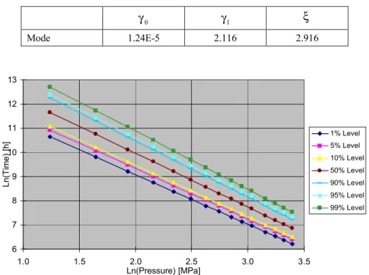
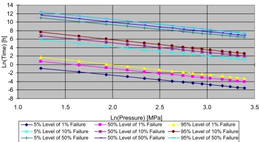
Figure 5 shows the predicted Life-Stress relationship for the Power-Weibull-Linear model with 95% probability intervals down to 40% stress level (Ln[Stress] = 3.32 MPa). Analyzing Figure 5, one can confirm the fact that the probability intervals become wider as the extrapolation is performed beyond the 40% stress level. Also, crossing percentiles are observed if extrapolation takes place at even lower stress levels as a consequence of such increase in uncertainty and wider probability intervals. Indeed, such fact is shown in Figure 6 where the predicted time percentiles for 1%, 10% and 50% failure fractions are estimated to the 10% stress level.

Such crossing percentiles result in longer life times for a lower failure fraction than at a higher one, which is physically implausible. For instance, the 5% probability level of 10% failure fraction at 10% stress level is Exp( 10.915 ) = 54995.13 hours, while the 95% probability level of 1% failure fraction at 10% stress level is Exp( 11.827 ) = 136899.18 hours (see Figure 6).

This fact indicates that the Power-Weibull-Linear model is inadequate for estimating failure times at extreme low stress levels. One possible approach to tackle this situation is to consider alternative testing plans in terms of testing unit allocation. For example, one could carry out tests at lower stress levels and testing more units at stress levels near the product service conditions. For an overview on accelerated life testing plans refer, for example, to Nelson (1990). For testing plan design from a Bayesian perspective see Chaloner & Larntz (1992), and for planning accelerated life tests under cost constrains see, for example, Tang & Xu (2005).

Table 1 – Data simulated via Monte Carlo.

Table 2 – Parameters values at the likelihood mode.

0

γ γ1 δ0 δ1

Input 5.0 1.5 0.7 0.4

Mode 5.1353 1.4447 0.7414 0.4974

6 7 8 9 10 11 12 13

1.5 2.0 2.5 3.0 3.5 4.0 4.5

Ln(Pressure) [MPa]

L

n

(T

im

e

)

[h

]

1% Level

5% Level

10% Level

50% Level

90% Level

95% Level

99% Level

Figure 3 – 1% Failure fraction as function of stress.

8 9 10 11 12 13 14

1.5 2.0 2.5 3.0 3.5 4.0 4.5

Ln(Pressure) [MPa]

L

n

(T

ime

)

[h

]

1% Level

5% Level 10% Level 50% Level 90% Level

95% Level 99% Level

Table 3 – Predicted 95% probability intervals for 50% and 1% failure fractions as function of stress.

Failure Fraction % Stress Level Ln[Time] (h) Time (h) Ln[Time] (h) Time (h) Ln[Time] (h) Time (h)

90% 8.85 6959.00 9.09 8878.00 8.96 7812.87

80% 9.05 8532.00 9.25 10410.00 9.15 9367.67 70% 9.26 10540.00 9.45 12760.00 9.35 11503.73 60% 9.47 13000.00 9.73 16740.00 9.59 14575.67 50% 9.70 16260.00 10.06 23480.00 9.87 19272.91 40% 9.95 21050.00 10.49 35820.00 10.21 27107.11

90% 6.62 746.80 7.26 1422.00 6.63 754.22

80% 6.87 958.50 7.47 1763.00 6.87 959.44

70% 7.14 1258.00 7.73 2273.00 7.14 1255.53

60% 7.44 1701.00 8.04 3098.00 7.44 1704.58

50% 7.76 2353.00 8.41 4509.00 7.80 2432.63

40% 8.14 3418.00 8.89 7290.00 8.22 3729.73

50%

1%

Lower Upper True Failure Fraction

Predicted Failure Fraction

6.0 6.5 7.0 7.5 8.0 8.5 9.0 9.5 10.0 10.5 11.0

3.3 3.4 3.5 3.6 3.7 3.8 3.9 4.0 4.1 4.2

Ln(Pressure) [MPa]

L

n

(T

ime

)

[h

]

5% Level of 1% Failure 50% Level of 1% Failure 95% Level of 1% Failure 5% Level of 10% Failure 50% Level of 10% Failure 95% Level of 10% Failure 5% Level of 50% Failure 50% Level of 50% Failure 95% Level of 50% Failure

6 7 8 9 10 11 12 13 14

1.9 2.4 2.9 3.4 3.9 4.4

Ln(Pressure) [MPa]

L

n

(T

ime

)

[h

]

5% Level of 1% Failure 50% Level of 1% Failure 95% Level of 1% Failure 5% Level of 10% Failure 50% Level of 10% Failure 95% Level of 10% Failure 5% Level of 50% Failure 50% Level of 50% Failure 95% Level of 50% Failure

Figure 6 – Predicted time percentiles for 1%, 10% and 50% failure fraction from 90% to 10% stress level.

4. Application: The Case of Pressure Vessels

The problem of stress-dependent life spread in accelerated life testing has been pointed out in the literature (see for instance Nelson, 1984). Barlow et al. (1988) presents a data set that is the result of a study of lifetimes of Kevlar/Epoxy Spherical Pressure Vessels subjected to constant sustained pressure until vessel failure known as stress-rupture. The experience with previous similar units and also with Kevlar 49/Epoxy strands leads to the conclusion that the lifetime of such pressure vessels is Weibull distributed, and the shape parameter is stress-dependent (Barlow et al., 1988). Although a stress-dependent shape parameter has been identified, no further modeling and analysis are presented toward the problem solution of predicting life at service conditions.

This section presents the analysis of the data set in (Barlow et al., 1988) under the Bayesian Power-Weibull-Linear model and predicts life percentiles for different failure fractions as a function of stress and extrapolating to lower stress levels representing service conditions. In order to allow for a comparative analysis, the pressure vessels data set is also analyzed considering a stress-independent shape parameter.

4.1 Pressure Vessels Data

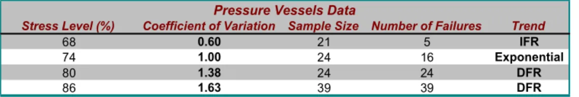
percentiles for 1%, 10% and 50% failure fraction at 50% stress level (2500 psig) and investigate further extrapolation to lower stress levels. As stated before, the lifetime of pressure vessels follows a Weibull distribution (Barlow et al., 1988). Table 4 shows the coefficient of variation based on maximum likelihood estimates of mean lifetime and standard deviation of lifetime. The estimates are based on a Weibull lifetime distribution. The column ‘trend’ indicates whether the time to failure distribution has decreasing failure rate (DFR), increasing failure rate (IFR) or approximately constant failure rate (exponential) at a given stress level.

From the analysis of the coefficient of variation shown in Table 4, one can make some preliminary observations about the failure rate function inside each stress level. Indeed, the failure rate is decreasing for the 86% and 80% stress levels, while it is approximately constant at 74% stress level, and increasing at lowest experimental stress of 68%. As stated by Barlow et al. (1988), the pressure vessels data indicate that the time the time to failure distribution shape parameter depends on the stress level. A more detailed data analysis of the data at each stress level can be found in Barlow et al. (1988).

Table 4 – Departure from exponentiality for the pressure vessels data.

Pressure Vessels Data

Stress Level (%) Coefficient of Variation Sample Size Number of Failures Trend

68 0.60 21 5 IFR

74 1.00 24 16 Exponential

80 1.38 24 24 DFR

86 1.63 39 39 DFR

4.2 Fitting the Power-Weibull Model with Stress-Independent Shape Parameter

To predict the posterior time percentiles at different stress levels assuming a constant shape parameter for the Weibull distribution it is necessary to obtain the posterior probability density function for the model parameters ξ γ γ, ₀, ₁ in equation (13). Given the considerable amount of available data, it is considered a flat prior distribution for the model parameters. Note that this is a conservative modeling option as it assumes no relevant prior information on the parameters. For cases dealing with small sample sizes, an informative prior distribution should be considered. For a detailed discussion about the construction of an informative prior distribution in the context of Weibull models see, for example, Groen & Droguett (2006).

Table 5 shows the parameter estimates at the likelihood mode. The Extreme Value scale parameter estimate at the mode is ξ =_M 2.916, which corresponds to a Weibull shape parameter of βM =1/ξM =0.343 indicating a decreasing failure rate in the region near the maximum likelihood. This result is somewhat expected as the most significant information is for higher stress levels, condition which is characterized by decreasing failure rates (see Table 4).

The 95% probability intervals are: 1.476E− <5 γ0<2.3817E−4, 2.1136< <γ1 2.3462,

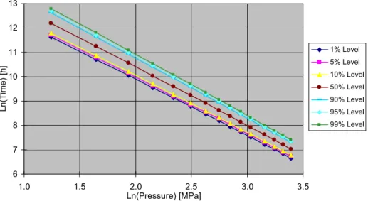
from almost zero (2.2 hours) to approximately 6177 hours at 86% and 80% stress levels, and these stresses are the ones with the higher number of failures. In Figure 7 is shown the time percentiles at various stress levels for 50% failure fraction (in Ln scales). It can be observed that as the stress decreases the uncertainty bounds become wider. The same fact is observed among different failure fractions, where the 95% probability interval at 50% failure fraction, for example, is narrower than the 95% probability interval at 10% and 1% failure fractions, as shown in Figure 8.

Figure 8 shows the 95% probability intervals of the time percentiles as function of stress ranging from 90% stress level to 10% stress level for three different failure fractions. As expected, the curves for different percentage points are parallel as a result of a stress-independent shape parameter.

Table 5 – Parameter estimates at the likelihood mode for the Power-Weibull model with stress-independent shape.

0

γ γ1 ξ

Mode 1.24E-5 2.116 2.916

6 7 8 9 10 11 12 13

1.0 1.5 2.0 2.5 3.0 3.5

Ln(Pressure) [MPa]

L

n

(T

ime

)

[h

]

1% Level

5% Level

10% Level

50% Level

90% Level

95% Level

99% Level

-8 -6 -4 -2 0 2 4 6 8 10 12 14

1.0 1.5 2.0 2.5 3.0 3.5

Ln(Pressure) [MPa]

L

n

(T

ime

)

[h

]

5% Level of 1% Failure 50% Level of 1% Failure 95% Level of 1% Failure

5% Level of 10% Failure 50% Level of 10% Failure 95% Level of 10% Failure

5% Level of 50% Failure 50% Level of 50% Failure 95% Level of 50% Failure

Figure 8 – Time percentiles as function of stress for 1%, 10% and 50% failure fractions under the Power-Weibull model with stress-independent shape.

4.3 Fitting the Power-Weibull Model with Stress-Dependent Shape Parameter

The pressure vessels data sets are now modeled according to the Power-Weibull-Linear model which has posterior parameters pdf given by equation (15). Once again, it was solved considering a flat prior pdf. The parameters mode estimates are: γ =₀ 1.3533E-25,

1 2.2459

γ = , δ =0 9.022E-28, δ =1 0.1205.

Observe that as in the previous case of constant shape, the parameter γ₀ has a very small value, indicating the data behavior of very small failure times at high stress levels. However, in the present situation, the shape parameter is considered as a linear function of the log (base e) stress. The parameter δ₀ shows a small value at the mode. Thus, for the pressure vessels data sets, both scale and shape parameters are expected to range from near zero at high stress levels based on the present state of knowledge provided by the available evidence. Further observations can be made analyzing the 95% Bayesian probability intervals for the model parameters: 1.54E-35<γ₀<1.66E-34, 2.1352< <γ₁ 2.3679,

0

1.339E-35<δ <5.0325E-35, 0.1017< <δ1 0.1323. The 95% probability interval of the δ1 does not include the zero value. Thus this coefficient, which defines the linear dependency between the shape parameter and stress, is significantly (convincingly) different from zero and hence ( )β s depends on stress in this model. Further insights will be given via application of the Likelihood Ratio test in the next section.

shape parameter is a linear function of the log stress. Indeed, the time percentiles tend to approximate to each other as the stress is decreased, and one would expect that they will cross each other at very low pressures. However, even extrapolating down to the 10% stress level (3.4591 MPa), the percentiles do not cross (see Figure 12). This fact is associated with this particular set of data which not only have a fairly large sample sizes but also a high number of failures.

6 7 8 9 10 11 12 13

1.0 1.5 2.0 2.5 3.0 3.5

Ln(Pressure) [MPa]

L

n

(T

ime

)

[h

]

1% Level

5% Level

10% Level

50% Level

90% Level

95% Level

99% Level

Figure 9 – Time percentiles as a function of stress for the 50% failure fraction under the Power-Weibull model with stress-dependent shape.

2 3 4 5 6 7 8 9 10 11

1.0 1.5 2.0 2.5 3.0 3.5

Ln(Pressure) [MPa]

L

n

(T

ime

)

[h

]

1% Level

5% Level

10% Level

50% Level

90% Level

95% Level

99% Level

-4 -2 0 2 4 6 8

1.0 1.5 2.0 2.5 3.0 3.5

Ln(Pressure) [MPa]

L

n

(T

ime

)

[h

]

1% Level

5% Level

10% Level

50% Level

90% Level

95% Level

99% Level

Figure 11 – Time percentiles as a function of stress for the 1% failure fraction under the Power-Weibull model with stress-dependent shape.

-6 -4 -2 0 2 4 6 8 10 12 14

1.0 1.5 2.0 2.5 3.0 3.5

Ln(Pressure) [MPa]

L

n

(T

ime

)

[h

]

5% Level of 1% Failure 50% Level of 1% Failure 95% Level of 1% Failure

5% Level of 10% Failure 50% Level of 10% Failure 95% Level of 10% Failure

5% Level of 50% Failure 50% Level of 50% Failure 95% Level of 50% Failure

5. Comparison of the Models

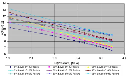
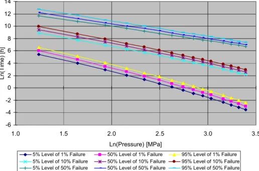
As shown in Figure 13, Figure 14 and Figure 15, the resulting uncertainty bounds for different time percentiles for various failure fractions (1%, 10% and 50%, respectively) for the Power-Weibull model with constant shape parameter are wider than the ones for the Power-Weibull-Linear model.

Another aspect to note is the form of the percentiles curves. For the model with stress-independent shape the curves are parallel to each other at different stress levels, but they present a curvature at high stress levels and tend to approximate to each other at lower pressures for the stress-dependent case. For the pressure vessels data, however, they do not cross at very low pressures.

In examining the fit of the Power-Weibull-Linear model to the pressure vessels data, it was checked whether the probability interval for the δ₁ parameter enclosed the zero value. If it does not enclose zero, one can conclude that the coefficient differs from zero, that is, a nonzero coefficient provides a convincing improvement in the fit of the model to the data. This procedure, however, may be misleading when the coefficient estimates are statistically correlated, and they usually are.

-6 -4 -2 0 2 4 6 8

1.0 1.5 2.0 2.5 3.0 3.5

Ln(Pressure) [MPa]

L

n

(T

im

e

)

[h

]

Stress Ind. 5% Level of 1% Failure Stress Ind. 50% Level of 1% Failure

Stress Ind. 95% Level of 1% Failure Stress Dep. 5% Level of 1% Failure

Stress Dep. 50% Level of 1% Failure Stress Dep. 95% Level of 1% Failure

1 2 3 4 5 6 7 8 9 10 11

1.0 1.5 2.0 2.5 3.0 3.5

Ln(Pressure) [MPa]

L

n

(T

im

e

)

[h

]

Stress Ind. 5% Level of 10% Failure Stress Ind. 50% Level of 10% Failure

Stress Ind. 95% Level of 10% Failure Stress Dep. 5% Level of 10% Failure

Stress Dep. 50% Level of 10% Failure Stress Dep. 95% Level of 10% Failure

Figure 14 – Comparison for time percentiles as function of stress for 10% failure fractions under the Power-Weibull model with stress-independent versus stress-dependent shape models.

6 7 8 9 10 11 12 13

1.0 1.5 2.0 2.5 3.0 3.5

Ln(Pressure) [MPa]

L

n

(T

im

e

)

[h

]

Stress Ind. 5% Level of 50% Failure Stress Ind. 50% Level of 50% Failure

Stress Ind. 95% Level of 50% Failure Stress Dep. 5% Level of 50% Failure

Stress Dep. 50% Level of 50% Failure Stress Dep. 95% Level of 50% Failure

The Likelihood Ratio Test (DeGroot & Schervish, 2002) is another way to deciding which coefficients to include in the model, i.e., whether the δ1 parameter is important in order to obtain an improved fit for the pressure vessels data. The log likelihood ratio test statistic for comparing the fit of two models with k and k′ parameters, respectively, is

2[max max ]

T= L− L′ where T has a Null distribution that is approximately χ2 with k−k′

degrees of freedom, and maxL is the maximum log likelihood. The maximum log likelihood for the case of stress-independent shape parameter is maxL′ = −242.396, and for the case of linear shape is maxL= −238.6574. Then, the statistic to test if the linear coefficient δ1 for the shape parameter differs from zero is T = −2[ 238.657 ( 242.396)]− − =

7.478 . As four coefficients are estimated for the Power-Weibull-Linear model and three coefficients for the model with constant shape parameter, one has that the χ2 95% percentile

with one degree of freedom is χ2(95%,1)=3.841. The calculated T statistic exceeds this critical value, hence δ1 is statistically significant at the 5% level. Furthermore, one can

observe that the T statistic also exceeds the 1% confidence level (χ2(99%,1)=6.635). Thus, the coefficient δ1 significantly improves the fit.

What are the implications on the product life at service conditions given prediction from the stress-independent and stress-dependent models? To answer this question, one can inspect Table 6 that shows the median estimates and corresponding uncertainty bounds (5% and 95% percentiles) of failure times at two product service conditions (50% stress level = 2500 psig, and 40% stress level = 2000 psig) for 1%, 10% and 50% failure fractions. Observe that, for the pressure vessel data, the stress-independent model consistently underestimates the time to failure across all the failure fractions compared to the estimates given by the stress-dependent model. Take the 50% failure fraction as an example. The median estimate of the failure time at 50% stress level (2500 psig) given the stress-independent model is 3193.9 hours, and 4315.6 hours for the stress-dependent model. The same behavior prevails for 10% and 1% failure fractions, with median failure times of 25.0 hours (10% failure fraction) and 0.06 hour (1% failure fraction), and 91.8 hours (10% failure fraction) and 0.7 hour (1% failure fraction) for the stress-independent and stress-dependent models, respectively.

Many are the implications of the lifetime underestimation at service conditions. For instance, it would undoubtedly imply in higher cost for the manufacturer as at one end it would offer more conservative warranty policies, and at the other end it would, for example, lead to unnecessary and unrealistic maintenance policies (e.g., shorter than necessary inspection intervals) and spare parts inventory.

Table 6 – Time to failures predictions at two service conditions for 1%, 10% and 50% failure fractions (time in hours).

Model 50% Stress Level (2,500 psig) 40% Stress Level (2,000 psig) Failure

Fraction

5% 50% 95% 5% 50% 95%

Indep. 0.01 0.06 0.13 0.02 0.10 0.22

1%

Dep. 0.4 0.7 1.3 1.2 2.0 3.5

Indep. 10.5 25.0 46.8 16.9 41.3 78.3

10%

Dep. 60.3 91.8 137.0 125.2 192.5 292.9

Indep. 1919.8 3193.9 5486.2 3071.7 5218.7 8955.3 50%

Dep. 3010.9 4315.6 6002.9 5064.4 7405.7 10829.2

6. Concluding Remarks

The Bayesian model presented in this paper allows for the modeling of accelerated life testing data that show stress-dependent spread in life, i.e., the failure mechanism is not equal for different stress levels. The model has been developed under the assumptions of Weibull distributed failure times, shape parameter as a linear function of the log stress, and scale parameter related to stress via the Power Law. However the modeling procedure can be applied, in principle, to any family of parametric distributions and functional forms for the relationships of scale and spread parameters and stresses. The Bayesian model has been validated through the use of simulated data (failure and censored times) via Monte Carlo, and its application to a real world scenario illustrated by using a previously published data.

References

(1) Bagdonavicius, V. & Nikulin, M. (2002). Accelerated Life Models, Modeling and Statistical Analysis. Chapman and Hall/CRC, Boca Raton.

(2) Barlow, R.; Toland, R. & Freeman, T. (1988). A Bayesian Analysis of the Stress-Rupture Life of Kevlar/Epoxy Spherical Pressure Vessels. In: Accelerated Life Testing and Experts’ Opinions in Reliability. Proceedings of the International School of Physics “Enrico Fermi”, Course CII.

(3) Carlsson, B.; Möller, K.; Köhl, M.; Heck, M.; Brunold, S.; Frei, C.; Marechal, J. & Jorgensen (2004). The Applicability of Accelerated Life Testing for Assessment of Service Life of Solar Thermal Components. Solar Energy Materials & Solar Cells, 84, 255-274.

(4) Chaloner, K. & Larntz, K. (1992). Bayesian Design for Accelerated Life Testing. Journal of Statistical Planning and Inference, 33, 245-259.

(5) DeGroot, M.H. & Schervish, M.J. (2002). Probability and Statistics. Third Edition, Addison Wesley.

(6) Fishman, G.S. (2000). Monte Carlo, Concepts, Algorithms and Applications. Springer.

(7) Gaertner, G.; Raasch, D.; Barratt, D. & Jenkins, S. (2003). Accelerated Life Tests of CRT Oxide Cathodes. Applied Surface Science, 215, 72-77.

(8) Groen, F. & Droguett, E.L. (2006). Prior Specification for Multi-Failure Mode Weibull Reliability Models. IEEE Reliability, Availability, Maintainability Symposium, California, USA.

(9) Groen, F. & Droguett, E.L. (2005). Competing Failure Mode Modeling in a Bayesian Reliability Assessment Tool. IEEE Reliability, Availability, Maintainability Symposium, Alexandria – VA, USA.

(10) Groen, F.; Droguett, E.L.; Jiang, S. & Mosleh, A. (2004). A Reliability Data Collection and Analysis System for Products under Development. Brazilian Journal of Operations Production Management, 1, 93-106.

(11) Gumbel, E.J. (1958). Statistics of Extremes. Colombia University Press, New York.

(12) Kececioglu, D. (1993). Reliability and Life Testing Handbook. Englewood Cliffs, NJ, Prentice-Hall.

(13) Koo, H.J. & Kim, Y.K. (2005). Reliability Assessment of Seat Belt Webbings through Accelerated Life Testing. Polymer Testing, 24, 309-315.

(14) Meeker, W.Q. & Escobar, L.A. (1998). Statistical Methods for Reliability Data. John Wiley, New York.

(15) Nelson, W. (1984). Fitting of Fatigue Curves with Nonconstant Standard Deviation to Data with Runouts. Journal of Testing and Evaluation, 12, 69-77.

(16) Nelson, W. (1982). Applied Life Data Analysis. John Wiley and Sons, New York.

(18) Tang, L.C. & Xu, K. (2005). A Multiple Objective Framework for Planning Accelerated Life Tests. IEEE Transactions on Reliability, 54 (1), 58-63.

(19) Tobias, P.A. & Trindade, D.C. (1995). Applied Reliability. 2nd edition, New York, Van Nostrand Reinhold.

(20) Weibull, W. (1951). A Statistical Distribution Function of Wide Applicability. Journal of Applied Mechanics. 18, 293-297.

(21) Whitman, C.S. (2003). Accelerated Life Test Calculations Using the Method of Maximum Likelihood: An Improvement over Least Squares. Microelectronics Reliability, 43, 859-864.

Appendix

In this appendix is presented the Pressure Vessels Accelerated Life Testing Data obtained from Barlow et al. (1988). Note that Type 0 means failure time and Type 1 means censored time.

Table 7 – Kevlar 49/Epoxy pressure vessels data tested at 68% stress level.

68% Stress Level (3400 psig) (n = 21 k = 5)

Rank Time(h) Type

1 4000.00 0

2 5376.00 0

3 7320.00 0

4 8616.00 0

5 9120.00 0

6 13272.00 1

7 13272.00 1

8 13272.00 1

9 13272.00 1

10 13272.00 1

11 13272.00 1

12 13272.00 1

13 13272.00 1

14 13272.00 1

15 13272.00 1

16 13272.00 1

17 13272.00 1

18 13272.00 1

19 13272.00 1

20 13272.00 1

21 13272.00 1

Table 8 – Kevlar 49/Epoxy pressure vessels data tested at 74% stress level.

74% Stress Level

(3700 psig) (n = 24 k = 18) Rank Time(h) Type

1 225.20 0

2 503.60 0

3 1087.70 0

4 1134.30 0

5 1824.30 0

6 1920.10 0

7 2383.00 0

8 2442.50 0

9 3708.90 0

Table 9 – Kevlar 49/Epoxy pressure vessels data tested at 80% stress level.

80% Stress Level

(4000 psig) (n = 24 k = 24) Rank Time(h) Type

1 19.10 0

2 24.30 0

3 69.80 0

4 71.20 0

5 136.00 0

6 199.10 0

7 403.70 0

8 432.20 0

9 453.40 0

10 514.10 0

11 514.20 0

12 541.60 0

13 544.90 0

14 554.20 0

15 664.50 0

16 694.10 0

17 876.70 0

18 930.40 0

19 1254.90 0 20 1275.60 0 21 1536.80 0 22 1755.50 0 23 2046.20 0 24 6177.50 0

Table 10 – Kevlar 49/Epoxy pressure vessels data tested at 86% stress level.

86% Stress Level

(4300 psig) (n = 39 k = 39)

Rank Time(h) Type

1 2.20 0

2 4.00 0

3 4.00 0

4 4.60 0

5 6.10 0

6 6.70 0

7 7.90 0

8 8.30 0

9 8.50 0

10 9.10 0

11 10.20 0

12 12.50 0

13 13.30 0

14 14.00 0

15 14.60 0

16 15.00 0

17 18.70 0

18 22.10 0

19 45.90 0

20 55.40 0

21 61.20 0

22 87.50 0

23 98.20 0

24 101.00 0

25 111.40 0

26 144.00 0

27 158.70 0

28 243.90 0

29 254.10 0

30 444.40 0

31 590.40 0

32 638.20 0

33 755.20 0

34 952.20 0

35 1108.20 0

36 1148.50 0

37 1569.30 0

38 1750.60 0