A brief look at the least-squares approach as a classifier applied
to restricted-vocabulary speech recognition
Rodrigo Capobianco Guido
,∗,
Luciene Cavalcanti Rodrigues
ABSTRACT
In this letter, a speech recognition algorithm based on the least-squares method is presented. Particularly, the intention is to exemplify how such a traditional numerical technique can be applied to solve a signal processing problem that is usually treated by using more elaborated formulations.
Keywords: least-squares method; speech recognition; “intelligent” transfer functions.
c
2012 Darbose. All rights reserved.
1. Introduction
In this letter, the potential offered by the least-squares method (LSM) [1] to solve incompatible systems of linear equations (ISLE) is explored in order to create a technique for speech recognition [2]. Pre-ceded by a basic feature extraction step, LSM is used to solve an ISLE whose solution characterizes an “intelligent” transfer function (ITF) that transforms an n-dimensional input vector into a scalar value. According to this value, which corresponds to the algorithm output, it is possible to know which was the input spoken word.
The remainder of this work is organized as follows. A very brief review on LSM, plus some concepts related to speech recognition, are presented in section2. Based on such information, section3describes the proposed approach, then, section 4 presents tests and results, and, lastly, section 5 describes the conclusions.
2. Brief review of important concepts
2.1 The least-squares method to solve incompatible systems of linear equations
In order to solve an incompatible linear system ofM equations inN unknowns, beingM > N, the LSM [1] is one of the possible, and most used, approaches. Its definition, which is well-documented in the literature [1], implies that, in practice, the generic linear system
α1,1x1+α2,1x2+α3,1x3+...+αn,1xn = β1
α1,2x1+α2,2x2+α3,2x3+...+αn,2xn = β2
α1,3x1+α2,3x2+α3,3x3+...+αn,3xn = β3
... . . ,
... . .
... . .
α1,mx1+α2,mx2+α3,mx3+...+αn,mxn = βm
which can be expressed in matricial form as being
α1,1 α2,1 α3,1 ... αn,1
α1,2 α2,2 α3,2 ... αn,2
α1,3 α2,3 α3,3 ... αn,3
... ... ... ... ... ... ... ... ... ... ... ... ... ... ... α1,mα2,mα3,m... αn,m
| {z }
matrixA[·][·]
· x1 x2 x3 . . . xn
| {z }
vectorX[·]
= β1 β2 β3 . . . βm
| {z }
vectorB[·]
,
can be approximatelly solved by multipling its both sides by AT
[·][·], i.e., the transpose of A[·][·]. We
therefore have:
AT[
·][·]·A[·][·]·X[·]=A
T
[·][·]·B[·] ,
which corresponds to an N by N linear system. The exact solution of this last system is the best approximation, in the least-squares sense, to the incompatible original system. This methodology is adopted in this work as a part of the proposed approach.
2.2 Speech recognition and feature extraction
Speech recognition has been intensively studied during the last decades, as can be observed, for example, in [2]. Traditionally, speech recognition algorithms are based on Hidden Markov Models (HMMs) or neural networks [3], mainly, when there is a large set of speech utterances or words to be recognized. On the other hand, when a modest set of words is being considered, simpler procedures can be certainly adopted. This is the case explored in the current work.
Independent of the algorithm used to recognize the words, which require previous digitalization by a computer or a digital signal processing (DSP) hardware, there is always an n-dimensional vector, stored in the computer memory, that corresponds to the digitalized speech signal. The length of such a vector is not constant, being proportional to the length of the spoken word, to the time the speaker needs to sound such a word, and so on. Since each word corresponds to a vector of one particular dimension, i.e., with a particular length, the transfer function used to convert such a vector into a scalar value representing the spoken word should be adaptive, in order to deal with that fact. This adaptation is neither an easy task to be implemented nor is functional in practice.
Feature extraction is, most of the times, the technique used to solve the above-mentioned problem. This solution implies that a small set ofP numerical parameters, or characteristics,P being a constant integer, is used to represent each spoken word. Thus, the role of a feature extraction step is to transform an n-dimensional vector, of variable length, into a considerable smaller vector with P parameters. Ob-viously, such parameters should be representative of the original spoken words. Many possibilities exist, being energies and fractal dimensions, for example, valid choices, according to [2] and [4].
3. The proposed approach
The description of the proposed approach follows, in the form of an algorithm. The values ofW andT, mentioned in it, will be discussed later.
• BEGINNING
• STEP S1: Define a small set ofW words to be recognized. Then, by using a computer, a proper
• STEP S2: By using a computational tool, such as Matlab, read the wave files, importing their
raw data, i.e., their digitalized signals values, into V =W·T vectors;
• STEPS3: Normalize all the vectors so that they have zero mean and unitary standard deviations;
• STEP S4: For each vectorVi, (1≤i≤(W·T)), extract a total of 15 parameters, P1 to P15, as
follows:
– P1: the energy of the entire vector;
– P2 andP3: the energies of the first and the second halfs of the vector, respectively;
– P4toP7: the energies of the first, second, third, and fourth forths of the vector, respectively;
– P8 toP15: the energies of the first, second, ..., and eight eights of the vector, respectively;
The use of 15 parameters is just the choice adopted here.
• STEP S5: For each one of theW words, assign an integer value,qj, to be used as a label;
• STEP S6: In order to determine the proper weight, αk, for each parameter, establish, for each
W·T spoken word, one linear combination betweenαk and the parametersPi, i.e., a linear system so that:
P1,vector1 P2,vector1 ... P15,vector1
P1,vector2 P2,vector2 ... P15,vector2
P1,vector3 P2,vector3 ... P15,vector3
... ... ... ...
P1,vectorV(W·T) P2,vectorV(W·T) ... P15,vectorV(W·T)
· α1
α2
α3
... α15
!
= q1
q2
q3
... q(W·T)
!
.
• STEP S7: Since the system above is incompatible, apply the LSM to obtain an approximate
solution,{α1, ..., α15}, to it;
• STEP S8: In order to recognize a new unknown input word, apply the steps S2 to S4 to the
corresponding wave file. This produces a set of fifteen parameters which are the features of the
word. Then, calculate the value R=P15 i=1
αk·Pk, which is the algorithm output. The label qi that
is closest toR corresponds to the unknown input word.
END.
In the algorithm above, the sampling rate and the quantization chosen, i.e., at least 8000Hz, 16-bit, is the one necessary to preserve frequencies below 4000 Hz, according to Nyquist’s sampling theorem [2]. This range of frequencies corresponds to the one in which voice signals are concentrated. In addition,
the energy of a vectorY[·], i.e., E(Y[·]), mentioned above, consists simply in the sum C P
s=1
ys2, beingC
the length ofY[·].
In relation to the values of W and T, the expectation is that the product W ·T, which corresponds to the number of equations in the linear system, should be considerable greater than the number of parameters P, that is equals to 7 in the proposed algorithm. This is because the intention is to create a transfer function that is built considering many examples of each word. In some specific case that
4. Example tests and their corresponding results
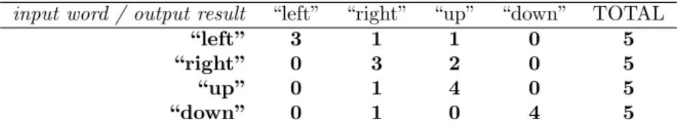
As an example situation,W = 4 was adopted, being “down”, “right”, “up”, and “left”, the correspond-ing words, and 0, 1, 2, and 3, their correspondcorrespond-ing labels, respectively. For each word, T = 5 utterances were collected from different speakers, including male, female, young, and elderly people. This totalizes 4·5 = 20 feature vectors of length fifteen each one. Carrying out the stepsS1 to S7 of the algorithm
presented in the previous section, the values ofα1 toα15 were determined.
In order to test the proposed technique, five additional utterances of each word were collected and the stepS8 of the algorithm was carried out. The results are listed in table1, which has the format of
a confusion matrix, in order to allow a more detailed description. As indicated in the table, the results
Table 1: results of the experiment.
input word / output result “left” “right” “up” “down” TOTAL
“left” 3 1 1 0 5
“right” 0 3 2 0 5
“up” 0 1 4 0 5
“down” 0 1 0 4 5
can be considered positive, since only some errors were detected, being the accuracy, i.e., the number of correct results in relation to the total number of words tested, equals to (3+3+4+4)(5+5+5+5) = 0.7 = 70%. Researchers or students interested in repeating the experiment, can contact the author, by e-mail, in order to obtain the material used.
5. Conclusions
This paper presented an interesting application of the LSM for restricted-vocabulary speech recognition. Although the LSM is a well-known technique in numerical analysis, its application in speech process-ing had never been showed before in literature in a so simple way. The proposed approach illustrated how one can construct an “intelligent” transfer function, by using basic mathematical tools, which trans-forms an input feature vector into a numerical output, making possible to recognize certain spoken words.
Of fundamental importance is the fact that no comparison between the proposed technique and other approaches for restricted-vocabulary speech recognition was presented. This is due to the fact that this work does not intend to improve any other existing technique which shows a better accuracy. Instead, the only intention is, as discussed above, to illustrate how a basic numerical tool can be applied to solve a practical problem in the field of signal processing. Researchers interested in more elaborated algorithms can consult, for example, the techniques presented in [2].
References
[1] Lawson, C.L.; Hanson, R.J.Solving Least Squares Problems (Classics in Applied Mathematics). Society for Industrial Mathematics Pub. Co., 1987.
[2] Coleman, J.,Introducing Speech and Language Processing. Cambridge: Cambridge University Press, 2005. [3] Haykin, S.Neural Networks and Learning Machines. 3 ed. Prentice-Hall, 2008.
[4] Al-Akaidi, M.Fractal speech processing. Cambridge-UK: Cambridge University Press, 2004.