Download details:
IP Address: 186.217.234.103
This content was downloaded on 10/10/2014 at 17:51
Please note that terms and conditions apply.
View the table of contents for this issue, or go to the journal homepage for more
A study of low velocities regions near the Roche lobe
during the gas giant planets formation
Ricardo A. Moraes
UNESP - Universidade Estadual Paulista, Guaratinguet´a, CEP 12516-110, SP, Brazil
E-mail: [email protected]
Ernesto Vieira Neto
UNESP - Universidade Estadual Paulista, Guaratinguet´a, CEP 12516-110, SP, Brazil
E-mail: [email protected]
Abstract. In this paper were studied regions close to the Roche lobe of a planet like Jupiter, in order to find regions with low velocities. We simulated a two dimensional and non-self-gravitating disk, where tidal and viscous torques are considered, using the hydrodynamic numerical integrator FARGO 2D. As stated earlier we are interested in find low velocities regions for in future works study the possibility of satellites formation in these regions.
1. Introduction
It’s believed that satellites of a giant gaseous planet were formed soon after the own planets, from material which was not accreted on the planet in its last formation phase. Our work analyzes some special regions near the Roche lobe of giant planets, regions where the gas has low velocities. We believe that these regions will occur accretive collisions between the material not accreted by planet and than, due to low velocity, a body could be formed. According to [6] the idea is that if the accreting inflow has sufficiently low angular momentum per unit mass, then the satellites formed with a circumplanetary disk will occupy a small region within the Hill sphere, such arguments justify our interest in the study these regions. Thus, we simulated the formation of a planet like Jupiter from a typical protoplanetary disk, using the core accretion model described in [1].
This work is structured as follows, in the section 2 we explain how a giant gaseous planet form according with the core accretion model. In the section 3 we describe the numerical procedures used in our simulation. In the section 4 we discuss about our results, in the section 5 we present the conclusions about the work, and in the section 6 comments about the next works that will arise from the results provided in this work.
2. Formation of Giant Gaseous Planets
Two teorical model are are frequently used to explain the formation of the giant gaseous planets, although they are not the only ones, the disk instability model and the core accretion model. From [1], the disk instability model for giant planet formation is predicated on the assumption that the gaseous protoplanetary disk was massive enough to be unstable in such a way that
accretion. In the first stage, the solid protoplanetary disk grows via a sucession of two-body collisions until it becomes massive enough to retain a significant gaseous atmosphere or envelope [1]. The process of formation of the planetary embryo requires, initially, low velocities in the collisions between the planetesimals, that are basically formed by rock and ice, on the feeding zone, assuming that the collisions between the planetesimals are totally accretive, that means, all the physical collisions are completely inelastic [5] we have that the initial solid core of the planet starts to form in this stage. That is considered a quick event, around 0.5 Myr after the formation of the star, and is similar to the formation of the terrestrial planets. The rate of planetesimals accretion can be calculated by [5]:
˙
Mcore=πR 2
σcoreΩFg (1)
where R is the radius of the accreting body,σcore is the surface density of planetesimals in the
solar nebula, Ω is the orbital frequency andFg is the gravitational enhancement factor.
In the second stage the protoplanet and the gaseous envelope are both in hydrostatic equilibrium, this equilibrium is broke when the protoplanet exceeds a critical mass due the constant accretion of material. The critical mass isn’t a constant, it’s a function of planetesimal accretion rate and opacity in the gaseous envelope, the estimates of the critical mass required range from 5M⊕ [2] to 20M⊕ or more [10]. From [1], the envelope opacities κR ≥10−2cm2g−1
the critical core mass can be approximated by:
Mcrit ≈7 (
˙
Mcore
10−7M ⊕yr−1
)q( κR
1cm2g−1
)s
M⊕ (2)
where q and sare both estimated to lie in the range 0.2-0.3
Once this mass is exceeded, the protoplanet enters in a stage called runaway growth, in this phase of the formation process there is no hydrostatic equilibrium, in other words, all material accumulated by the planet during the previous steps collapses to its core. For massive planets the most of its planetary envelope is accreted during this stage, which is a quick process, about 105
years.
In the final stage of the formation, the protoplanet do not accretes gas anymore, either as a consequence of the planet opening a local gap in the disk or as a consequence of the dissipation of the entire protoplanetary disk [1]. The energy released by accretion increases considerably the temperature of the planet and of its gaseous envelope, as a consequence, the icy planetesimals which were accreted dissolves causing the core to be composed only by the rocky material, ending the whole process of formation of a gas giant planet.
3. Numerical procedures
For the development of the numerical calculations we used the hydrodynamic numerical integrator FARGO 2D [8] and we set up our simulations in the conditions used in [7].
We simulated a two-dimensional protoplanetary disk, considering the tidal and viscous torques, with neglected self-gravity. A typical protoplanetary disk has a thickness of radius given by the ratio H/r ≈0.05−0.1 [7], we adopted a thickness to radius of the disk as H/r= 0.05 and non reflecting inner boundary conditions [4].
Figure 1. Scheme of formation of a giant planet via core accretion. Adapted from [1].
In our model we adopted the viscous forces per unit area of Navier-Stokes equations for modeling the viscous forces. The origin of the coordinate system is taken to be in the center of the star, and we used cilindrical coordinates (r, θ). Thus, the equations of motion are given by [7]:
∂Σ
∂t +∇(Σu) = 0 (3) ∂pr
∂t +∇(pru) = Σr (uθ
r + Ωp )2
−∂p
∂r −Σ
∂Φ
∂r +fr (4)
∂j
∂t +∇(ju) =− ∂p
∂θ −Σ
∂Φ
∂θ +fθ (5)
where Σ is the surface density of the disk, u is the flow velocities, in terms of its components, can be written by u = urˆr+uθθˆ, pr = Σur is the radial momentum per unit area, p is the
vertically integrated gas pressure, Ωp is the angular velocity of the planet,j = Σr(uθ+ Ωpr) is
the gas angular momentum per unit area, f=frrˆ+fθθˆis the viscous force per unit area and Φ
is the gravitational potential smoothed in the neighborhood of the planet, given by [7]:
Φ =−GMs
r −
GMp
(|r−rp|2+rsm2 ) 1 2
(6)
where Ms is the mass of the star, Mp is the mass of the planet, rp is the planet position and rsm is the smoothing length of the planet’s potential.
For the value of the kinematic turbulent viscosity we have,ν =µ/Σ, whereνcan be expressed in terms of the α prescription given in [11] as,
ν =αcsH (7)
where cs is the sound speed, H is the thickness of the protostellar disk and the parameterα is
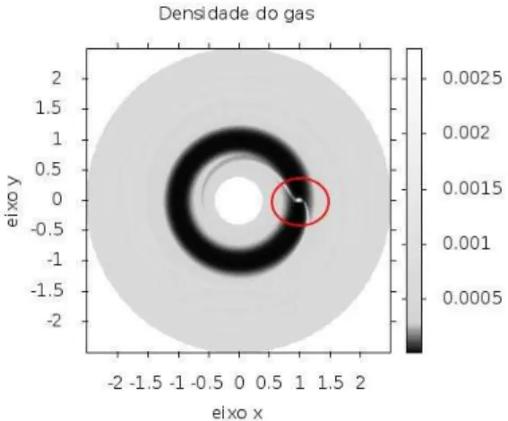
The figure 2.a shows the gas density in the simulated disk and inside the circle we have around the region of Roche lobe, in this figure we can see the gap opened by the planet.
The figure 2.b shows the region inside the circle of figure 2.a. We can clearly see the low density in two regions close to the planet, what can be an evidence of regions with low velocities that we are looking for, we can’t conclude this looking to this figure, for this we present the figure 3.
(a) Gas density in all region around the planet.
(b) Zoom aplied in the figure 2.a.
Figure 2. Gas density around the planet.
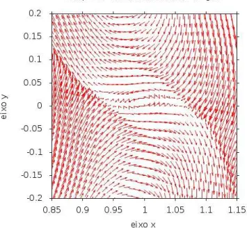
In figure 3 we show the velocity field around the simulated planet, this figure assists our analises about the velocities close to the planet. We see in this figure, that near the planet the velocities converges to the planet creating a vortex, we believe that this vortex could be responsable for the accretion of planetesimals. We also identified regions of escape of planetesimals, these regions have high velocities and pointing outward the center of the planet. There is also two peculiar regions in this figure, it is slightly above and below the vortex of the planet, in these regions we can observe that the velocities field is to weak, these regions are, indeed, the regions that we are looking for, which we called low velocities regions.
Figure 3. Velocities field around the planet.
5. Conclusions
With the simulations described in the previous sections we found the low velocities regions close to the Roche lobe of giant gaseous planet, as showed in figure 3. The results found in this work agrees with the results presented by [7] and [4], who analyzed these regions before. Besidesfinding the low velocities regions, we also obtained results that given us an estimation of the location of these regions
6. Future works
The results presented in this paper are preliminary results, our goal was show that there are regions with low velocities close to the Roche lobe of giant gasous planet. With this result, we will study the possibility of the satellite formation in these regions, the goal of the new project is to show that regions with low velocities close to the Roche lobe can be good sites to satellite formation, to do that, we must simulate planetesimals near to the planet, in the region of interest.
References
[10] Pollack, J. B., Hubickyj, O., Bodenheimer, P.,et al. 1996,Icarus12462 [11] Shakura, N. I., Sunyaev, R. A., 1973,Astronomy &Astrophysics 24337
![Figure 1. Scheme of formation of a giant planet via core accretion. Adapted from [1].](https://thumb-eu.123doks.com/thumbv2/123dok_br/16287734.185129/4.892.146.676.170.529/figure-scheme-formation-giant-planet-core-accretion-adapted.webp)