Global Discriminative Learning for
Higher-Accuracy Computational Gene Prediction
Axel Bernal1*, Koby Crammer1, Artemis Hatzigeorgiou2, Fernando Pereira11Department of Computer and Information Science, University of Pennsylvania, Philadelphia, Pennsylvania, United States of America,2Department of Genetics, University of Pennsylvania, Philadelphia, Pennsylvania, United States of America
Most ab initio gene predictors use a probabilistic sequence model, typically a hidden Markov model, to combine separately trained models of genomic signals and content. By combining separate models of relevant genomic features, such gene predictors can exploit small training sets and incomplete annotations, and can be trained fairly efficiently. However, that type of piecewise training does not optimize prediction accuracy and has difficulty in accounting for statistical dependencies among different parts of the gene model. With genomic information being created at an ever-increasing rate, it is worth investigating alternative approaches in which many different types of genomic evidence, with complex statistical dependencies, can be integrated by discriminative learning to maximize annotation accuracy. Among discriminative learning methods, large-margin classifiers have become prominent because of the success of support vector machines (SVM) in many classification tasks. We describe CRAIG, a new program for ab initio gene prediction based on a conditional random field model with semi-Markov structure that is trained with an online large-margin algorithm related to multiclass SVMs. Our experiments on benchmark vertebrate datasets and on regions from the ENCODE project show significant improvements in prediction accuracy over published gene predictors that use intrinsic features only, particularly at the gene level and on genes with long introns.
Citation: Bernal A, Crammer K, Hatzigeorgiou A, Pereira F (2007) Global discriminative learning for higher-accuracy computational gene prediction. PLoS Comput Biol 3(3): e54. doi:10.1371/journal.pcbi.0030054
Introduction
Prediction of protein-coding genes in eukaryotes involves correctly identifying splice sites and translation initiation and stop signals in DNA sequences. There are two main gene prediction methods. Ab initio methods rely exclusively on intrinsic structural features of genes, such as frequent motifs in splice sites and content statistics in coding regions. Notable ab initio predictors include GenScan [1], Augustus [2], TigrScan/Genezilla [3], HMMGene [4], GRAPE [5], MZEF [6], and Genie [7]. Homology-based methods exploit extrinsic features derived by comparative analysis. For instance, ProCrustes [8], GeneWise, and GenomeWise [9] exploit protein or cDNA alignments, while TwinScan [10], Double-Scan [11], and NDouble-Scan [12] rely on genomic DNA from related informant organisms. Extrinsic features improve the accuracy of predictions for genes with close homologs in related organisms. Krogh [13] and Mathe et al. [14] review current gene prediction methods.
GenScan was the first gene predictor to achieve about 80% exon sensitivity and specificity in several single-gene bench-mark test sets. More recent predictors have improved on GenScan’s results by focusing on specific aspects of gene prediction. For example, GenScanþþimproves specificity for internal exons and Augustus improves prediction accuracy on very long DNA sequences. Despite these advances, overall accuracy on chromosomal DNA, particularly in regions with low gene density (low GC content), is not yet satisfactory [15]. Gene-level accuracy, which is especially important for applications, is a major challenge.
Improvements at the gene level could have a positive impact on detecting gene-related biological features such as signal peptide regions, promoters, and even 39 UTR micro-RNA targets. Genes with very long introns and intergenic
regions represent more than 95% of the total number of genes in most vertebrate genomes, and even a small improve-ment on those could be significant in practice.
With the exception of MZEF, which uses a quadratic discriminant function to identify internal coding exons, all of the ab initio predictors mentioned above use hidden Markov models (HMMs) to combine sequence content and signal classifiers into a consistent gene structure. HMM parameters are relatively easy to interpret and to learn. Content and signal classifiers can be built effectively using a variety of machine learning and statistical sequence modeling methods. However, the combination of content and signal classifiers with the HMM gene structure model is not itself trained to maximize prediction accuracy, and the overall model does not fully account for the statistical dependencies among the features used by the various classifiers. Moreover, recent work on machine learning for structured prediction problems [16,17] suggests that global optimization of model parameters to minimize a suitable training criterion can achieve better
Editor:David Haussler, University of California Santa Cruz, United States of America
ReceivedAugust 16, 2006;AcceptedFebruary 1, 2007;PublishedMarch 16, 2007
A previous version of this article appeared as an Early Online Release on February 2, 2007 (doi:10.1371/journal.pcbi.0030054.eor).
Copyright:Ó2007 Bernal et al. This is an open-access article distributed under the terms of the Creative Commons Attribution License, which permits unrestricted use, distribution, and reproduction in any medium, provided the original author and source are credited.
Abbreviations:CRAIG, CRF-based ab initio genefinder; CRF, conditional random fields; HMM, hidden Markov model; MIRA, Margin Infused Relaxed Algorithm; PWM, position weight matrices; SVM, support vector machines; TIS, translation initiation site; WAM, weight array model; WWAM, windowed weight array model
results than separate training of the various components of a structured predictor.
To overcome the shortcomings outlined above, our gene predictor uses a linear structure model based on conditional random fields (CRFs) [17], hence the name CRAIG (CRF-based ab initio genefinder). CRFs are discriminatively trained Markovian state models that learn how to combine many diverse, statistically correlated features of the input to achieve high accuracy in sequence tagging and segmentation problems. Our models are semi-Markov [18] to model more accurately the length distributions of genomic regions. For training, instead of the original conditional maximum-like-lihood training objective of CRFs, we use the online large-margin MIRA (Margin Infused Relaxed Algorithm) method [19], allowing us to extend to gene prediction the advantages of large-margin learning methods such as support vector machines (SVMs) while efficiently handling very long training sequences. Figure 1 presents schematically the differences in the learning process between our method and the most common generative approach for gene prediction.
Our model and training method allow us to combine a rich variety of possibly overlapping genomic features and to find a global tradeoff among feature contributions that maximizes annotation accuracy. In particular, we model different types of introns according to their length, which would have been difficult to integrate in previous models. We were also able to include rich features for start and stop signals and globally balance their weights against the weights of all other model features. These advances led to significant overall improve-ments over the current best predictions for the most used benchmark test sets: sensitivity and specificity of initial and single exon predictions showed a relative mean increase [2] of 25.5% and 19.6%, respectively; at the gene level, the relative mean improvement was 33.9%; the relative F-score improve-ment on the ENCODE regions was 16.05% at the exon level. These improvements were in good part due to the different treatment of intronic states within the model, which in turn increased structure prediction accuracy, particularly on genes with long introns.
Some previous gene predictors have used discriminative
training to some extent. HMMGene uses a nongeneralized HMM model for gene structure, which does not include features associated with biological signals, but it is trained with the discriminative conditional maximum likelihood criterion [20]. However, conditional maximum likelihood is more difficult to optimize than our training criterion because it is required to respect conditional independence and normalization for the underlying HMM. GRAPE takes a hybrid approach for learning. It first trains parameters of a generalized HMM (GHMM) to maximize generative like-lihood, and then it selects a small set of parameters that are trained to maximize the percentage of correctly predicted nucleotides, exons, and whole genes used as surrogates of the conditional likelihood. This approach is commonly used when training data is limited, and it usually provides superior results only in those cases [21]. However, the GRAPE learning method does not globally optimize the training criterion.
Results
Datasets
All the experiments reported in this paper use a gene model trained on a nonredundant set of 3,038 single-gene sequences. We built this set by combining the Augustus training set [2], the GenScan training set, and 1,500 high-confidence CDSs from EnsMart Plus [22], which are part of the Genezilla training set (http://www.tigr.org/software/ traindata.shtml). We then appended simulated intergenic material to both ends of each training sequence to make up for the lack of realistic intergenic regions in the training material, as described in more detail in Methods.
We compared CRAIG with GenScan, TwinScan 2.03 (with-out homology features, also known as GenScanþþ), Genezilla (formerly known as TigrScan), and Augustus on several benchmark test sets. We also ran predictions with HMMGene, the only other publicly available genefinder to use a discriminative structure training method; we present some prediction results with it in Methods. All programs we compare with are based on similar GHMM models with similar sequence features. Augustus uses two types of length distributions for introns: short intron lengths are modeled with an explicit distribution, but other introns use the default geometric distribution. This difference made Augustus run many times slower than the other programs in all our experiments.
We evaluated the programs on the following benchmark test sets.
BGHM953. This test set combines most of the available
single-gene test sets in one single set. It includes the GeneParser I (27 genes) and II (34 genes) datasets [23], 570 vertebrate sequences from Burset and Guigo [24], 178 human sequences from Guigo et al. [25], and 195 human, rat, and mouse sequences from Rogic et al. [26]. Repeated entries were removed. We combined different sets to obtain more reliable evaluation statistics by smoothing out possible overfitting to particular sequence types.
TIGR251.This test set consists of 251 single-gene sequen-ces, which are part of the TIGR human test dataset (http:// www.tigr.org/software/traindata.shtml), and it is composed mostly of long-intron genes.
ENCODE294.This test set consists of 31 test regions from
the ENCODE project [27,28], for a total of 21M bases,
Author Summary
containing 294 carefully annotated alternatively spliced genes and 667 transcripts, after eliminating repeated entries and partial entries with coordinates outside the region’s bounds. This is the only test set that was masked using RepeatMasker (http://www.repeatmasker.org/) before performing gene pre-diction. Table 1 gives summary statistics for the training set and the three test sets.
Predictions on all tests and for all programs—including CRAIG—allow partial genes, multiple genes per region, and genes on both strands. Alternative splicing and genes embedded within genes were not evaluated in this work. Any other program parameters were left at their default values. For each program, we used the human/vertebrate gene models provided with the software distributions. In all tests, sequences with noncanonical splice sites were filtered out. Accuracy numbers were computed with the eval package [29], a standard and reliable way to compare different gene predictions.
Prediction in Single-Gene Sequences
Table 2 shows prediction results for all programs on
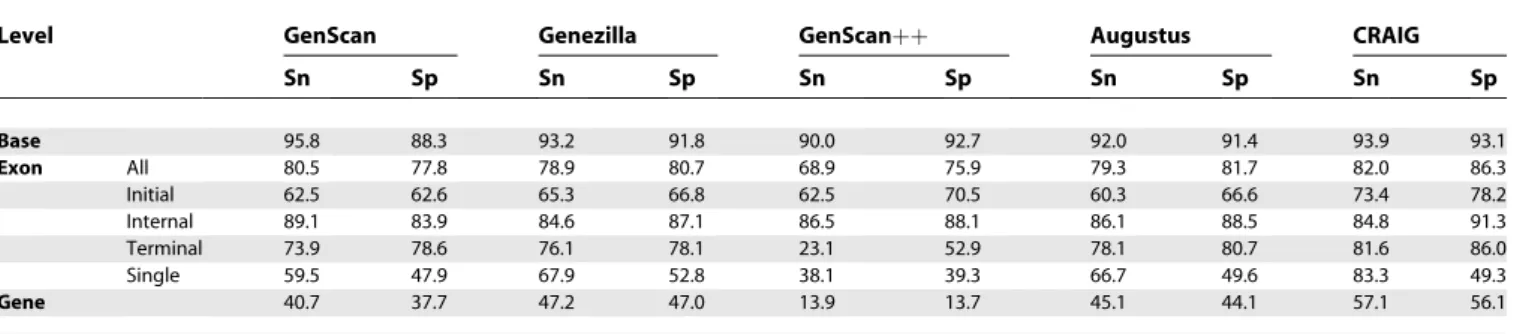
BGHM957. CRAIG achieved better sensitivity and specificity than the other programs at all levels, except for somewhat lower base sensitivity but much higher base specificity than GenScan. The relative F-score improvement for initial and single exons over Genezilla, the second-best program overall for this set, was 14.6% and 5.8%, respectively. Single-exon genes were more difficult to predict for all programs, with specificity barely exceeding 50% for the best program, but CRAIG’s relative improvement in sensitivity was nearly 25%
over runner-up Genezilla. Terminal exon predictions were also improved over the nearest competitors, but less markedly so. The improved gene-level accuracy follows from these gains at the exon level. GenScanþþ and Augustus predicted internal exons with similar accuracy and their F-scores were only slightly worse than CRAIG, but the overall gene-level accuracy for GenScanþþlooks much worse because it missed many terminal and single exons. GenScan also did well in this set, but overall performance was somewhat worse than the other programs.
Most of the genes in this set have short introns and the intergenic regions are truncated, so prediction was relatively easy and all programs did relatively well. The next section compares performance on datasets with long-intron genes and very long intergenic regions.
Prediction in Long DNA Sequences
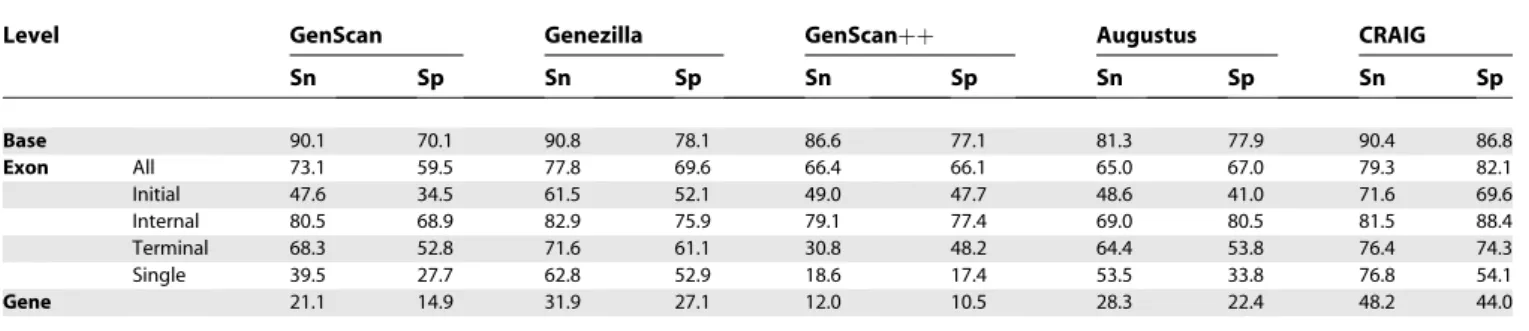
As previously noted, TIGR251 has many genes with very
long introns, so it is expected to be harder to predict accurately. This was confirmed by the results in Table 3. Performance was worse for all programs and levels when compared with the first set. However, CRAIG consistently outperformed the other programs with an even wider performance gap than in the first experiment. Here, base and internal-exon accuracies were also substantially im-proved. CRAIG’s relative F-score improvement for bases and internal exons over Genezilla, the second-best program in both categories, was 5.4% and 7.1%, respectively, compared with approximately 1% for BGHM953. Other types of exons also improved, as in the first experiment.
Figure 1.Learning Methods: Discriminative versus Generative
Schematic comparison of discriminative (A) and generative (B) learning methods. In the discriminative case, all model parameters were estimated simultaneously to predict a segmentation as similar as possible to the annotation. In contrast, for generative HMM models, signal features and state features were assumed to be independent and trained separately.
Because of these better base and exon-level predictions, the relative F-score improvement over runner-up Genezilla at the gene level was about 57%.
Our final set of experiments was on ENCODE294. The
results are shown in Table 4. As previously mentioned, all sequences in this set were masked for low-complexity regions and repeated elements. Unlike previous sets, in which masking did not affect results significantly, prediction on unmasked sequences in this set was worse for all programs (unpublished data). In particular, exon and base specificity decreased an average of 8%.
We added a transcript-level prediction category to Table 4 to better evaluate predictions on alternatively spliced genes. We closely followed the evaluation guidelines and definitions by Guigo and Reese [28]. There, transcript and gene-level predictions that are consistent with annotated incomplete transcripts are counted correct, even in cases where the predictions include additional exons. We relaxed this policy to also mark as correct those predictions that contained incomplete transcripts whose first (last) exon did not begin (end) with an acceptor (donor). The reason for this change is that no program can exactly predict both ends of such transcripts. We developed our own programs to evaluate single-exon, transcript, and gene-level predictions for in-complete transcripts. Evaluations for other categories and for complete transcripts were handled directly with eval.
To ensure consistency in the evaluation, we obtained all of the programs except for Genezilla from their authors and we ran them on the test set in our lab. Genezilla predictions for
this set were obtained directly from the supplementary material provided by [28] so that we could measure the potential differences between our evaluation method and that reported in [28], particularly at the transcript and gene level, for which we expected different results.
Overall, our results for all programs agree with those of Guigo and Reese [28]. Genezilla’s base and exon-level results using our evaluation program closely matched the published values. Transcript and gene-level results computed by our method were 1% better than the published numbers, which roughly match the percentage of incomplete annotated transcripts with no splice signals on either end. Computed predictions for GenScan and Augustus were also somewhat different, but not substantially so, from those reported by Guigo and Reese [28], presumably because of differences in program version and operating parameters.
Improvements in this set were similar to those obtained in our second experiment. The relative F-score improvements for individual bases and internal exons were 6% and 15.4% over GenScanþþ and Augustus, the runner-ups in each respective category. Improvement in prediction accuracy on single, initial, and terminal exons is similar to that for the other test sets. Transcript and gene-level accuracies were, respectively, 30% and 30.6% better than Augustus, the second-best program overall. This means that our better accuracy results obtained in the first two single-gene sequence sets scale well to chromosomal regions with multi-ple, alternatively spliced genes.
Table 1.Dataset Statistics
Dataset Number of Exons
Number of Genes
Single Exon Genes
Coding (Percent)
Average Number of Exons
Average Coding Length (bp)
Average Transcript Length (bp)
Average Intron Length (bp)
Training 17,875 3,038 721 6.8 6.27 1,213 17,683 3,119
BGHM953 4,544 953 84 24.9 4.77 860 3,453 687
TIGR251 1,496 251 43 5.8 5.96 1,044 17,857 3,389
ENCODE294 2,842 294 65 4.6 8.3 1,305 28,179 4,094
BGHM953is a standard benchmark set of single-gene sequences with high protein-coding content (;23%), short average transcript length (;3,000 bp), and short average intron length (;700 bp).TIGR251is also a single-gene sequence set but transcripts and introns are longer; genes in this set resemble our training set the most.BGHM953, and to some extent TIGR251, are not representative of the whole human genome, because of their high relative frequencies of single-exon genes and coding loci. In contrast,ENCODE294is a highly curated dataset containing multiple-gene sequences with long intergenic regions and alternatively spliced genes with long introns. These characteristics more closely resemble real chromosomal DNA. Results onENCODE294may thus be better estimates of performance on biologically interesting genomic sequences.
doi:10.1371/journal.pcbi.0030054.t001
Table 2.Accuracy Results forBGHM953
Level GenScan Genezilla GenScanþþ Augustus CRAIG
Sn Sp Sn Sp Sn Sp Sn Sp Sn Sp
Base 95.8 88.3 93.2 91.8 90.0 92.7 92.0 91.4 93.9 93.1
Exon All 80.5 77.8 78.9 80.7 68.9 75.9 79.3 81.7 82.0 86.3
Initial 62.5 62.6 65.3 66.8 62.5 70.5 60.3 66.6 73.4 78.2
Internal 89.1 83.9 84.6 87.1 86.5 88.1 86.1 88.5 84.8 91.3
Terminal 73.9 78.6 76.1 78.1 23.1 52.9 78.1 80.7 81.6 86.0
Single 59.5 47.9 67.9 52.8 38.1 39.3 66.7 49.6 83.3 49.3
Gene 40.7 37.7 47.2 47.0 13.9 13.7 45.1 44.1 57.1 56.1
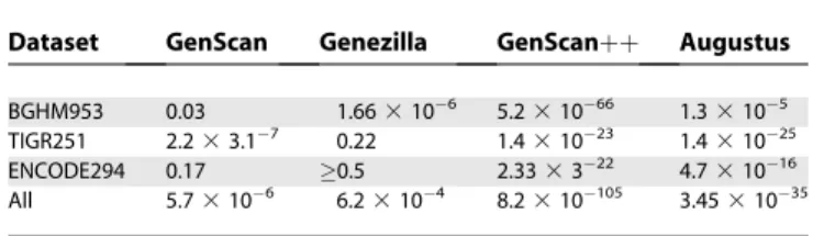
Significance Testing
In all tests and at all levels, CRAIG achieved greater improvements in specificity than in sensitivity. We inves-tigated whether the improvements in exon sensitivity achieved by CRAIG could be explained by chance. Any exon belonging to a particular test set is associated with two dependent Bernoulli random variables for whether it was correctly predicted by CRAIG and by another program. We computed p-values with McNemar’s test for dependent, paired samples from CRAIG and each of the other programs over the three test sets, as shown in Table 5. The null hypothesis was that CRAIG’s advantage in exon predictions is due to chance. Thep-values were,0.05 for all entries, except
for the TIGR251 experiments against Genezilla and the
ENCODE294experiments against Genezilla and GenScan; in
general, these two genefinders proved to be very sensitive at the cost of predicting many more false positives.p-Values for the combined test sets were all below 0.001, showing that CRAIG’s advantage was extremely unlikely to be a chance event.
We also trained and tested an additional variant of CRAIG, in which we did not distinguish between short and long introns; this configuration corresponds closely to the state model representation used in most previous works. Following Stanke and Waack [2], we used the relative mean improve-ment:
r¼DSnexonþDSpexonþDSngeneþDSpgene
4 ð1Þ
as the measure of differences in prediction accuracy between the CRAIG variant and CRAIG itself. The term DSnexon
denotes the mean increase in exon sensitivity and is defined as
DSnexon¼
X
t2T
nt3DSntexon
X
t2T
nt
wherentis the number of annotated genes in datasett, T¼
fBGHM953, TIGR251, ENCODE294g, and DSntexon is the
difference in exon sensitivity between CRAIG and the CRAIG variant on dataset t. The other terms are defined similarly. The improvement obtained by CRAIG with respect to the variant wasr¼3.6. This result was as expected: there was an improvement in accuracy from including the extra intron state in the gene model, but even the simpler variant was more than competitive with the best current genefinders.
Discussion
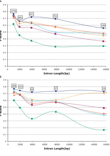
It is well-known that more gene prediction errors occur on regions with low GC content, which have higher intron and intergenic region density [15]. This behavior can also be observed on our combined results, as shown in Figure 2A. It also can be noticed that CRAIG had the best F-score for all intron lengths. Except for CRAIG and HMMGene, the F-scores for all other predictors were very close for all lengths. CRAIG’s advantage over its nearest competitors became more
Table 3.Accuracy Results forTIGR251
Level GenScan Genezilla GenScanþþ Augustus CRAIG
Sn Sp Sn Sp Sn Sp Sn Sp Sn Sp
Base 90.1 70.1 90.8 78.1 86.6 77.1 81.3 77.9 90.4 86.8
Exon All 73.1 59.5 77.8 69.6 66.4 66.1 65.0 67.0 79.3 82.1
Initial 47.6 34.5 61.5 52.1 49.0 47.7 48.6 41.0 71.6 69.6
Internal 80.5 68.9 82.9 75.9 79.1 77.4 69.0 80.5 81.5 88.4
Terminal 68.3 52.8 71.6 61.1 30.8 48.2 64.4 53.8 76.4 74.3
Single 39.5 27.7 62.8 52.9 18.6 17.4 53.5 33.8 76.8 54.1
Gene 21.1 14.9 31.9 27.1 12.0 10.5 28.3 22.4 48.2 44.0
Sensitivity (Sn) and specificity (Sp) for each level and exon type. doi:10.1371/journal.pcbi.0030054.t003
Table 4.Accuracy Results forENCODE294
Level GenScan Genezilla GenScanþþ Augustus CRAIG
Sn Sp Sn Sp Sn Sp Sn Sp Sn Sp
Base 84.0 62.1 87.6 50.9 76.7 79.3 76.9 76.1 84.4 80.8
Exon All 59.6 47.7 62.5 50.5 51.6 64.8 52.1 63.6 60.8 72.7
Initial 28.0 23.5 36.4 25.0 25.5 47.8 34.7 38.1 37.3 55.2
Internal 72.6 54.3 73.9 63.2 68.0 62.8 59.1 74.7 71.7 81.2
Terminal 33.0 31.6 36.7 28.5 25.7 53.9 37.6 45.5 33.3 52.6
Single 28.1 31.0 44.1 14.5 35.0 45.7 43.9 25.5 55.9 26.4
Transcript 8.1 11.4 10.3 9.9 6.0 17.0 10.9 16.9 13.5 23.8
Gene 16.7 11.4 20.6 9.9 12.5 17.0 22.3 16.9 26.6 23.8
apparent as introns increased in length. However, all gene-finders experience a significant drop in accuracy, at least 25% between 1,000 bp and 16,000 bp. For introns shorter than 1,000 bp, Augustus performs almost as well as CRAIG, in part because of its more complex, time-consuming model for short intron lengths.
Intron analysis of individual test sets, as shown in Figure 2B–2D, reveals that, except for ENCODE294, CRAIG con-sistently achieved an intron F-score above 75%, even for
lengths more than 30,000 bp; in contrast, the F-scores of all other programs fell to lower than 65%, even for introns as short as 8,000 bp. The results show that CRAIG predicts genes with long introns much better than the other programs. This hypothesis was also confirmed with experiments on an edited version ofENCODE294in which the original 31 regions were split into 271 contig sequences and all of the intergenic material was deleted except for 2,000 bp on both sides of each gene. This edited version was further subdivided into subsets with—ALT_ENCODE155—and without— NOALT_EN-CODE139—alternative splicing. Figure 3 shows intron pre-diction results for this arrangement. It can be observed that intron prediction onNOALT_ENCODE139, a subset of 139
genes, has the same characteristics as either TIGR251 or
BGHM953, that is, a rather flat F-score curve as intron length
increases. The same cannot be said about complementary subsetALT_ENCODE155, whose significant drop in accuracy for long introns can be explained by the presence of alternative splicing.
We claimed in the Introduction that a key aspect of our model and training method is the ability to combine various genomic features and to find a global tradeoff among their
Figure 2.F-Score as a Function of Intron Length
Results for all sets combined (A) and for individual test sets shown in subfigures (B–D). The boxed number appearing directly above each marker represents the total number of introns associated with the marker’s length. For example, there were 1,475 introns with lengths between 1,000 and 2,000 base pairs for all sets combined (A).
doi:10.1371/journal.pcbi.0030054.g002 Table 5.Significance Testing
Dataset GenScan Genezilla GenScanþþ Augustus BGHM953 0.03 1.663106 5.231066 1.33105 TIGR251 2.233.17 0.22 1.431023 1.431025 ENCODE294 0.17 0.5 2.333322 4.731016 All 5.73106 6.23104 8.2310105 3.4531035
McNemar test results (p-value upper bounds) of paired exon sensitivity predictions between CRAIG and each of the other programs.
contributions so that accuracy is maximized. Being able to identify introns longer than 30,000 bp with prediction accuracy comparable to that achieved on smaller introns is evidence that our program does a better job of combining features to recognize structure. Another way to see how well features have been integrated into the structure model is to examine signal predictions. It is well-known that translation initiation sites (TIS) are surrounded by relatively poorly conserved sequences and are harder to predict than the highly conserved splice signals. Also, stop signals present almost no sequence conservation at all and their prediction depends solely upon how well the last acceptor (in multi-exon genes) or the TIS (in single-exon genes) was predicted. Therefore, a simple splice site classifier can perform fairly well using only local sequence information. In contrast, TIS and stop signal classifiers are known to be much less accurate. Given these observations, we expected CRAIG to improve the most on TIS signal prediction accuracy, as all other programs examined in this work use individual classifiers for signal prediction, whereas CRAIG uses global training to compute each signal’s net contribution to the gene structure. Figure 4 shows the improvement in signal prediction accuracy for CRAIG when compared with the second-best program in each case. CRAIG shows improvement for all types of signals,
but the improvement was most marked for TIS, especially in specificity. It can also be observed that the improvement on stop signals follows from the co-occurring improvement on both acceptor and TIS signals. The final outcome is that CRAIG makes fewer mistakes in deciding where to start translation and stop translation, which is one of the main reasons for its significant improvement at the gene level.
There is great potential for including additional informa-tive features into the model without algorithm changes, for instance, features derived from comparative genomics. To facilitate such extensions, we designed CRAIG to allow model changes without recompiling the Cþþtraining and test code. The finite-state model, the features, and their relationships to states and transitions are all specified in a configuration file that can be changed without recompiling the program. This flexibility could be useful for learning gene models on organisms that may require a different finite-state model or a different set of features.
Materials and Methods
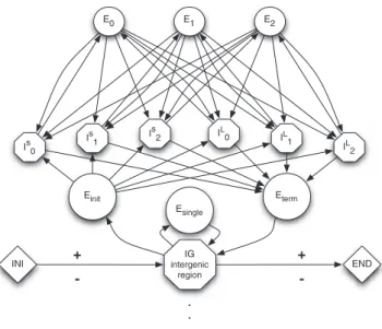
Gene structures.In what follows, a gene structure consists of either a single exon or a succession of alternating exons and introns, trimmed from both ends at the TIS and stop signals. We distinguish two different types of introns: short—980 bp or less—and long— more than 980 bp. Figure 5 shows a gene finite-state model that implements these distinctions.
Linear structure models.In what follows,x¼x1. . .xPis a sequence
ands¼s1. . .sQis a segmentation ofx, where each segmentsj¼ hpj,lj,yji
starts at position pos(sj)¼pj, has length len(sj)¼lj, and state label lab(sj)
¼yj, with pjþ1¼pjþlj P and 1 lj B for some empirically
determined upper bound B. The training data. t¼ fðxðtÞ
;s
ðtÞÞgT t¼1
consists of pairs of a sequence and its preferred segmentation. For
DNA sequences,xi2RDNA¼ fA, T, G, Cg, and each label lab(sj) is one
of the states of the model (Figure 5). A segment is also referred to as a genomic region; that is, an exon, an intron, or an intergenic region. A first-order Markovian linear structure model computes the score
of a candidate segmentations¼s1. . .sQof a given input sequencexas
a linear combination of terms for individual features of a candidate segment, the label of its predecessor, and the input sequence. More
precisely, each proposed segmentsjis represented by a feature vector
f(sj,lab(sj1),x) 2 <D computed from the segment, the label of the
previous segment, and the input sequence around position pos(sj). A
weight vector,w2 <D, to be learned, represents the relative weights of
the features. Then, the score of candidate segmentation s for
sequencexis given by
Figure 3.F-Score versus Intron Length for the Encode Test Set Results in subfigures (A) and (B) correspond to the subset of alternatively spliced genes and its complementary subset, respectively.
doi:10.1371/journal.pcbi.0030054.g003
Figure 4.Signal Accuracy Improvements
CRAIG’s relative improvements in prediction specificity (orange bar) and sensitivity (blue bar) by signal type. In each case, the second-best program was used for the comparison: Genezilla for starts, Augustus for stops, and GenScanþþfor splice sites.
Swðx;sÞ ¼
X
Q
j¼1
wfðsj;labðsj1Þ;xÞ ð2Þ
For gene prediction, we need to answer three basic questions. First,
given a sequence, x, we need to efficiently find its best-scoring
segmentation. Second, given a training set t¼ fðxðtÞ
;s
ðtÞÞgT t¼1, we
need to learn weightswsuch that the best-scoring segmentation ofx(t)
is close tos(t). Finally, we need to select a feature functionfthat is suitable for answering the first two questions while providing good generalization to unseen test sequences. The next three subsections answer these questions.
Inference for gene prediction.LetGEN(x)be the set of all possible
segmentations ofx. The best segmentation ofxfor weight vectorwis
given by:
^
s¼arg max
s2GENðxÞSwðx;sÞ ð3Þ
We can compute^sefficiently fromxusing the following
Viterbi-like recurrence:
Mði;yÞ ¼
maxy9;1lminfi;BgMðil;y9Þþ
wfðhil;l;yi;y9;xÞ
0
‘
ifi.0 ifi¼0 otherwise 8
> > <
> > :
ð4Þ
It is easy to see thatMði;yÞ ¼maxs2GENi;yðxÞSwðx;sÞ;where GENi,y(x)
is the set of all segmentations of x1. . .xi that end with label y.
Therefore, Sw(x,sˆ) ¼ M(P þ 1,END), where END is a special
synchronization state inserted at position P þ 1. The actual
segmentations are easily obtained by keeping back-pointers from each state-position pair (y,i) to its optimal predecessor (y9,il). The
complexity of this algorithm isO(PBm2), wheremis the number of
distinct states andB is the upper bound on the segment length,
because the runtime ofwfis independent ofP, B,orm. To reduce
the constant factor from these dot product computations, mostwf
values are precomputed and cached. For introns and intergenic
regions, the feature function f is a sum of per-nucleotide
contributions, so the dynamic program in Equation 4 needs only
to look at position i 1 when y corresponds to such regions.
Therefore,B needs to be only the upper bound for exon lengths,
which was chosen following Stanke and Waack [2]. For long sequences, the complexity of the inference algorithm is therefore
dominated by the sequence lengthP.
Online large-margin training.Online learning is a simple, scalable, and flexible framework for training linear structured models. Online algorithms process one training example at a time, updating the model weights to improve the model’s accuracy on that example.
Large-margin classifiers, such as the well-known SVMs, provide strong theoretical classification error bounds that hold well in practice for many learning tasks. MIRA [30] is an online method for training large-margin classifiers that is easily extended to structured problems [19]. Algorithm 1 shows the pseudocode for the MIRA-based training
algorithm we used for our models. For each training sequence,x(t), the
algorithm seeks to establish a margin between the score of the correct segmentation and the score of the best segmentation according to the current weight vector that is proportional to the mismatch between the candidate segmentation and the correct one. MIRA keeps the norm of the change in weight vector as small as possible while giving the current example (x(t),s(t)) a score that exceeds that of the best-scoring incorrect segmentation by a margin given by the mismatch between the correct segmentation and the incorrect one. The quadratic program in line 5 of Algorithm 1 formalizes that objective, and has a straightforward closed-form solution for this version of the
algorithm. Line 11 of the algorithm computeswas an average of the
weight vectors obtained at each iteration, which has been shown to
reduce weight overfitting [31]. The training parameter N is
determined empirically using an auxiliary development set. Algorithm 1.Online Training Algorithm.
Training datat¼ fðxðtÞ
;s
ðtÞÞgT
t¼1.L(s(t),sˆ) is some nonnegative
real-valued function that measures the mismatch between segmentationsˆ
and the correct segmentation s(t). The number of rounds
N is
determined using a small development set.
1: w(0)¼0;v¼0;i¼0
2: forround¼1 toNdo
3: fort¼1 toTdo
4: ^s¼arg maxs2GENðxÞSwðiÞðxðtÞ;sÞ
5: ^w¼arg minw9jjw9wðiÞjj2
subject toSw9(x(t),s(t))Sw9(x(t),sˆ)L(s(t),sˆ) 6: w(iþ1) wˆ
7: v vþw(iþ1)
8: i iþ1
9: end for 10: end for 11: w¼v/ (N*T)
Successful discriminative learning depends on having training data with statistics similar to the intended test data. However, this is not the case for gene training data. The main distribution mismatch is that reliable gene annotations available for training are for the most part for single-gene sequences with very small flanking intergenic regions.
To address this problem, we created long training sequences composed of actual genes separated by synthetic intergenic regions as follows. For each training sequence, we generated two extra inter-genic regions and appended them to both sequence ends, making sure that the total length of both flanking intergenic regions followed geometric distributions with means 5,000, 10,000, 60,000, and 150,000 bp for each of four GC content classes, respectively [3,10]. The synthetic intergenic regions were generated by sampling from GC-dependent, fourth-order interpolated Markov models (IMMs), with the same form as the models we used to score the intergenic state.
Algorithm 1 also requires a loss function, L, and a small
development set on which to estimate the number of rounds,N. As
loss function, we used the correlation coefficient at the base level [24], since it combines specificity and sensitivity into a single measure. The development set consisted of the 65 genes previously used in GenScan [1] to cross-validate splice signal detectors.
Features.The final ingredient of the CRAIG model is the feature
functionfused to score candidate segments based on properties of
the input sequence. A typical feature relates a proposed segment to some property of the input around that segment, and possibly to the label of the previous segment.
Properties.We started by introducing basic sequence properties that
features are based on. These properties are real-valued functions of the input sequence around a particular position. Some properties represent tests, taking the binary values 1 for true and 0 for false. For
any testP,||P|| denotes the function with value 1 if the test is true, 0
otherwise. The tests
subuði;xÞ ¼
jj
u¼x½i : iþ juj 1jj
Figure 5.Finite-State Model for Eukaryotic Genes
Variable-length genomic regions are represented by states, and bio-logical signals are represented by transitions between states. Short and long introns are denoted by ISand IL, respectively.
check whether substringuoccurs at positioni2x. For example,x¼
ATGGCGGA would have subA(1,x)¼1, subTA(2,x)¼0, and subGGC(3,x)
¼1.
The property scorey(i,x) computes the score of a content model for
stateyat positioni. This score is the probability that nucleotideihas
labelyaccording to ak-order interpolated Markov model [32], where
k¼8 for coding states andk¼4 for noncoding states.
The property gcc(i,x) calculates the GC composition for the region
containing position i, averaged over a 10,000-bp window around
positioni.
Each feature associates a property to a particular model state or state transition.
Binning.Properties with multimodal or sparse distributions, such as
segment length, cannot be used directly in a linear model, because their predictive effect is typically a nonlinear function of their value. To address this problem, we binned each property by splitting its range into disjoint intervals or bins, and converting the property into a set of tests that checked whether the value of the property belonged to the corresponding interval. The effect of this transformation was to pass the property through a stepwise constant nonlinearity, each step corresponding to a bin, where the height of each step was learned as the weight of a binary feature associated to the appropriate test.
For example, following GenScan [1], we mapped the GC content
property gcc to four bins:,43, 43–51, 51–57, and.57. For other
properties, we used regular bins with a property-specific bin width. For instance, exon length was mapped to 90 bp–wide bins.
Test and feature combinations.We used Boolean combinations of tests
and binary features to model complex dependencies on the input. Conjunctions can model nucleotide correlations, for example donors
of the form G1G5, that is, donors with G at positions1 and 5.
Likewise, disjunctions were used to model consensus sequences, for example, donors of the form U3, that is, donors with either an A or a G at position 3.
In general, for two binary functions f andg, we denoted their
conjunction byf^gand their disjunction byf_g.
State features.State features encode the content properties of the genomic regions associated to states: exons, introns, and intergenic regions. State features do not depend on the previous state, so we omitted the previous state argument in these feature definitions.
Coding/noncoding potential.This feature corresponds to the log of the probability assigned to the region by the content scoring model:
potðs;xÞ ¼
1 lenðsÞ
X posðsÞþlenðsÞ
k¼posðsÞ
log scorelabðsÞðk;xÞ llabðsÞ
wherelyis the arithmetic mean of the distribution of log scoreyon
the training data. For coding regions, the sum is computed over codon scores instead of base scores. Other features related to log
scoreyalso included infare the coding differential and the score
log-ratios between intronic and intergenic regions.
Phase biases.Biases in intron and exon phase distributions have
been found and analyzed by Fedorov et al. [33]. We represented possible biases with the straightforward functions
biaspðs;xÞ ¼ jjlabðsÞ ¼Ipjj
wherep¼0,1,2 is a phase and Ipis the corresponding intronic state.
Length distributions. The length distributions of exons and introns
have been extensively studied. Raw exon lengths were binned to allow our linear model to learn the length histogram from the training
data. For long introns, with length.980, we used 980/len(s) as the
length feature, whereas shorter introns used maxf245/len(s),1g.
For each genomic region type, we also provided length-dependent default features whose weights expressed a bias for or against regions
of that length and type. The value of these features is len(s)/ky, where
kyis the average length of ally-labeled segments. For introns and
intergenic regions, we used separate, always-on default features for the four classes of GC content discussed above.
Coding composition. In addition to coding potential scores, which
give broad, smoothed statistics for different genomic region types, we also defined count features for each 3-gram (codon) and 6-gram (bicodon) in an exon, and similar count features for the first 15 bases (five codons) of an initial exon. The 3-gram features were further split by GC content class. The general form of such a feature is
countu;pðs;xÞ ¼
X posðsÞþm
i¼posðsÞþp
subuði;xÞ if labðsÞ¼Ep
0 otherwise
8 > > <
> > :
wherep¼0,1,2 is the phase,uis the n-gram, andmis the window size,
which is len(s) for a general exon count, and minflen(s),15gfor special initial exon features, which attempt to capture composition regularities right after the TIS.
Masking.We represented the presence of tandem repeats and other
low complexity regions in exonic segments by the function:
maskðs;xÞ ¼
jj
1 lenðsÞ
X
posðsÞþlenðsÞ
k¼posðsÞ
subNði;xÞ.0:5
jj
After training, this feature effectively penalizes any exon whose
fraction ofNoccurrences exceeds 50% of its total length.
Table 6 shows all the state features associated with each segment label.
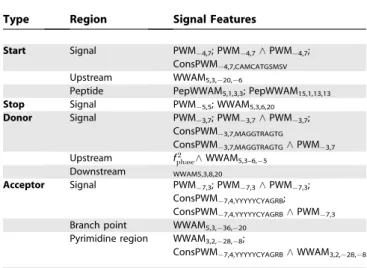
Transition features.Transition features look at biological signals that indicate a switch in genomic region type. Features testing for those signals looked for combinations of particular motifs within a window centered at a given offset from the position where the transition occurs. Features of the following form, which test for motif occurrence, are the building blocks for the transition features: Table 6.State Features for Each Segment Label
Segment Label Category State Features
Intergenic Length len(s)/ky
Score pot(s,x)
Intron Short only maxf980/len(s),1glen(s)/ky Long only 980/len(s)/kylen(s)/ky Phase biasp(s,x)
Score pot(s,x)
Exon Length bins len(s)ky
Content mask(s,x) countu,p(s,x) Score pot(s,x)
This summary elides some dependencies of features on state labels. For example, the feature pot(s,x) would behave differently depending on whethersis an intron, exon, or
intergenic segment, as described in the text. doi:10.1371/journal.pcbi.0030054.t006
Table 7.Transition Features per Signal Type
Type Region Signal Features
Start Signal PWM4,7; PWM4,7^PWM4,7;
ConsPWM4,7,CAMCATGSMSV Upstream WWAM5,3,20,6
Peptide PepWWAM5,1,3,3; PepWWAM15,1,13,13 Stop Signal PWM5,5; WWAM5,3,6,20
Donor Signal PWM3,7; PWM3,7^PWM3,7;
ConsPWM3,7,MAGGTRAGTG
ConsPWM3,7,MAGGTRAGTG^PWM3,7
Upstream f2
phase^WWAM5,3–6,5 Downstream WWAM5,3,8,20
Acceptor Signal PWM7,3; PWM7,3^PWM7,3;
ConsPWM7,4,YYYYYCYAGRB;
ConsPWM7,4,YYYYYCYAGRB^PWM7,3 Branch point WWAM5,3,36,20
Pyrimidine region WWAM3,2,28,8;
ConsPWM7,4,YYYYYCYAGRB^WWAM3,2,28,8
motifp;u;wðs;y9;xÞ ¼
X
w
2
d¼w
2
subuðposðsÞ þpþd;xÞ
wherepis the offset,wis the window width, anduis the motif. This
feature counts the number of occurrences ofuwithinp6w/2 bases of
the start of segments.
In principle, all sequence positions are potential signal occur-rences, but in practice one might filter out unlikely sites, using a sensitivity threshold proportional to level of signal conservation, thus decreasing decoding time.
Burge and Karlin [1] model positional biases within signals with combinations of position weight matrices (PWMs) and their general-izations, weight array models (WAMs) and windowed weight array models (WWAMs), with very good results. It is straightforward to
define these models as sets of features based on our motifp,u,wfeature,
as shown here in the WWAM case:
WWAMw;n;q;rðs;y9;xÞ ¼ fmotifp;u;wðs;y9;xÞ:u2
Xn
DNA
;qprg ð5Þ
PWMs and WAMs are special cases of WWAMs and can thus be
defined by PWMq,r¼WWAM1,1,q,r and WAMq,r¼WWAM1,2,q,r. This
means that we can use all of these techniques to model biological signals in CRAIG with the added advantage of having all signal model parameters trained as part of the gene structure.
Correlations between two positions within a signal are captured by conjunctions of motif features. For example, the feature conjunction
motif3;A;1ðh156;20;I1i;E1;xÞ ^motif2;T;1ðh156;20;I1i;E1;xÞ
would be 1 whenever there is an A in position3 and a T in position 2
relative to a donor signal occurring at position 156 in x, and 0
otherwise.
We can also extend the feature conjunction operator to sets of
features: ifAandBare sets of features, such as the WWAM defined in
Equation 5, we can define the set of featuresA^B¼ ff^g:f2A, g2Bg.
In Equation 5, if we use the amino acid alphabetP
AAinstead of
PDNA, and work with codons instead of single nucleotides, we can model signal peptide regions. If we sum over disjunctions of motif features, we can easily model consensus sequences.
Table 7 shows the motif feature sets for each biological signal. The parameters required by each feature type were either taken from the literature [1] or by search on the development set.
We included an additional feature set, motivated by previous work [2], to learn splice site information from sequences that only contain intron annotations. For any donor (acceptor), we first counted the number of similar donors (acceptors) in a given list of introns. A signal was considered to be similar to another if the Hamming distance between them was at most 1. The features were induced by a logarithmic binning function applied over the total number of similarity counts for Hamming distances 0 and 1.
Acknowledgments
We thank Aaron Mackey for advice on evaluation methods, datasets, and software.
Author contributions.AB, AH, and FP conceived and designed the experiments. AB performed the experiments and analyzed the data. AB and FP wrote the paper. AB, KC, and FP contributed ideas to the model and algorithms and refined and implemented the algorithms. FP proposed the initial idea.
Funding.This material is based on work funded by the US National Science Foundation under ITR grants EIA 0205456 and IIS 0428193 and Career grant 0238295.
Competing interests.The authors have declared that no competing interests exist.
References
1. Burge CB, Karlin S (1998) Finding the genes in genomic DNA. Curr Opin Struct Biol 8: 346–354.
2. Stanke M, Waack S (2003) Gene prediction with a hidden Markov model and a new intron submodel. Bioinformatics 19 (Supplement 2): II215–II225. 3. Majoros WH, Pertea M, Salzberg SL (2004) TigrScan and GlimmerHMM: Two open source ab initio eukaryotic genefinders. Bioinformatics 20: 2878–2879.
4. Krogh A (1997) Two methods for improving performance of an HMM and their application for gene finding. Proc Int Conf Intell Syst Mol Biol 5: 179–186.
5. Majoros WH, Salzberg SL (2004) An empirical analysis of training protocols for probabilistic genefinders. BMC Bioinformatics 5: 206.
6. Zhang MQ (1997) Identification of protein coding regions in the human genome by quadratic discriminant analysis. Proc Natl Acad Sci U S A 94: 565–568.
7. Kulp D, Haussler D, Reese MG, Eeckman FH (1996) A generalized hidden Markov model for the recognition of human genes in DNA. Proc Int Conf Intell Syst Mol Biol 4: 134–142.
8. Gelfand MS, Mironov AA, Pevzner PA (1996) Gene recognition via spliced sequence alignment. Proc Natl Acad Sci U S A 93: 9061–9066.
9. Birney E, Clamp M, Durbin R (2004) Genewise and genome wise. Genome Res 14: 988–995.
10. Korf I, Flicek P, Duan D, Brent MR (2001) Integrating genomic homology into gene structure. Bioinformatics 17 (Supplement 1): S140–S148. 11. Meyer IM, Durbin R (2002) Comparative ab initio prediction of gene
structures using pair HMMs. Bioinformatics 18: 1309–1318.
12. Gross SS, Brent MR (2005) Using multiple alignments to improve gene prediction. J Comput Biol 13: 379–393.
13. Krogh A (1998) Gene finding: Putting the parts together. In: Bishop M, editor. Guide to human genome computing. San Diego: Academic Press. pp. 261–274.
14. Mathe C, Sagot MF, Schiex T, Rouze P (2002) Current methods of gene prediction, their strengths and weaknesses. Nucleic Acids Res 30: 4103–4117. 15. Flicek P, Keibler E, Hu P, Korf I, Brent MR (2003) Leveraging the mouse genome for gene prediction in human: From whole-genome shotgun reads to a global synteny map. Genome Res 13: 46–54.
16. Ra¨tsch G, Sonnenburg S, Srinivasan J, Witte H, Mu¨ller KR, et al. (2007)
Improving theC. elegansgenome annotation using machine learning. PLoS
Comput Biol 3: e20.
17. Lafferty J, McCallum A, Pereira F (2001) Conditional random fields: Probabilistic models for segmenting and labeling sequence data. In: Danyluk A, editor. Proceedings of the Eighteenth International Conference
on Machine Learning; 28 June–1 July, 2001; Williamsburg, Massachusetts, United States. ICML ’01. San Francisco: Morgan Kauffman. pp. 282–289. 18. Sarawagi S, Cohen WW (2005) Semi-Markov conditional random fields for
information extraction. In: Saul LK, Weiss Y, Bottou L, editors. Adv in Neur Inf Proc Syst 17. Cambridge (Massachusetts): MIT Press. pp. 1185–1192. 19. Crammer K, Dekel O, Keshet J, Shalev-Shwartz S, Singer Y (2006) Online
passive–aggressive algorithms. J Machine Learning Res 7: 551–585. 20. Juang B, Rabiner L (1990) Hidden Markov models for speech recognition.
Technometrics 33: 251–272.
21. Raina R, Shen Y, Ng AY, McCallum A (2004) Classification with hybrid generative/discriminative models. In: Thrun S, Saul LK, Scho¨lkopf B, editors. Adv in Neur Inf Proc Syst 16. Cambridge (Massachusetts): MIT Press. pp. 545–552.
22. Kasprzyk A, Keefe D, Smedley D, London D, Spooner W, et al. (2004) Ensmart: A generic system for fast and flexible access to biological data. Genome Res 14: 160–169.
23. Snyder EE, Stormo GD (1995) Identification of protein coding regions in genomic DNA. J Mol Biol 248: 1–18.
24. Burset M, Guigo R (1996) Evaluation of gene structure prediction programs. Genomics 34: 353–357.
25. Guigo R, Agarwal P, Abril JF, Burset M, Fickett JW (2000) An assessment of gene prediction accuracy in large DNA sequences. Genome Res 10: 1631–1642.
26. Rogic S, Mackworth AK, Ouellette FB (2001) Evaluation of gene-finding programs on mammalian sequences. Genome Res 11: 817–832.
27. ENCODE Project Consortium (2004) The ENCODE (Encyclopedia of DNA Elements) project. Science 306: 636–540.
28. Guigo R, Reese MG, editors (2006) Egasp ’05: Encode genome annotation assessment project. Genome Biology 7 (Supplement 1).
29. Keibler E, Brent MR (2003) Eval: A software package for analysis of genome annotations. BMC Bioinformatics 4: 50.
30. Crammer K (2004) Online learning of complex categorical problems [Ph.D. thesis]. Jerusalem: Hebrew University.
31. Collins M (2002) Discriminative training methods for hidden Markov models: Theory and experiments with perceptron algorithms. In: Proceedings of Conference on Empirical Methods in Natural Language Processing; 6–7 July 2002; Philadelphia, Pennsylvania, United States. EMNLP 2002. pp. 1–8. 32. Salzberg SL, Delcher A, Kasif S, White O (1998) Microbial gene
identification using interpolated Markov models. Nucleic Acids Res 26: 544–548.