for Microarray Data Classification
Shiquan Sun, Qinke Peng*, Adnan Shakoor
Systems Engineering Institute, School of Electronic and Information Engineering, Xi’an Jiaotong University, Xi’an, China
Abstract
High dimensionality and small sample sizes, and their inherent risk of overfitting, pose great challenges for constructing efficient classifiers in microarray data classification. Therefore a feature selection technique should be conducted prior to data classification to enhance prediction performance. In general, filter methods can be considered as principal or auxiliary selection mechanism because of their simplicity, scalability, and low computational complexity. However, a series of trivial examples show that filter methods result in less accurate performance because they ignore the dependencies of features. Although few publications have devoted their attention to reveal the relationship of features by multivariate-based methods, these methods describe relationships among features only by linear methods. While simple linear combination relationship restrict the improvement in performance. In this paper, we used kernel method to discover inherent nonlinear correlations among features as well as between feature and target. Moreover, the number of orthogonal components was determined by kernel Fishers linear discriminant analysis (FLDA) in a self-adaptive manner rather than by manual parameter settings. In order to reveal the effectiveness of our method we performed several experiments and compared the results between our method and other competitive multivariate-based features selectors. In our comparison, we used two classifiers (support vector machine,k-nearest neighbor) on two group datasets, namely two-class and multi-class datasets. Experimental results demonstrate that the performance of our method is better than others, especially on three hard-classify datasets, namely Wang’s Breast Cancer, Gordon’s Lung Adenocarcinoma and Pomeroy’s Medulloblastoma.
Citation:Sun S, Peng Q, Shakoor A (2014) A Kernel-Based Multivariate Feature Selection Method for Microarray Data Classification. PLoS ONE 9(7): e102541. doi:10.1371/journal.pone.0102541
Editor:Andrew R. Dalby, University of Westminster, United Kingdom
ReceivedApril 7, 2014;AcceptedJune 20, 2014;PublishedJuly 21, 2014
Copyright:ß2014 Sun et al. This is an open-access article distributed under the terms of the Creative Commons Attribution License, which permits unrestricted use, distribution, and reproduction in any medium, provided the original author and source are credited.
Data Availability:The authors confirm that all data underlying the findings are fully available without restriction. All relevant data within the paper can be downloaded for free. The MATLAB source code of kernelPLS is publicly available at https://github.com/sqsun/kernelPLS
Funding:This work was jointly supported by the National Natural Science Foundation of China (grant numbers 61173111, 60774086) and the Ph. D. Programs Foundation of Ministry of Education of China (grant number 20090201110027). The funders had no role in study design, data collection and analysis, decision to publish, or preparation of the manuscript.
Competing Interests:The authors have declared that no competing interests exist. * Email: [email protected]
Introduction
Microarray gene expression based cancer classification is one of the most important tasks in bioinformatics. A typical classification task is to separate healthy patients from cancer patients, based on their gene expression ‘‘profile’’. However, because cancers are usually marked by changing in the expression levels of certain genes [1], therefore it is obvious that not all measured features are discriminative features for target. Hence, feature selection problem is ubiquitous in cancer classification.
Feature selection techniques for microarray data can be broadly grouped into three categories that are wrapper (classifier-dependent) methods [2,3], embedded (classifier-(classifier-dependent) meth-ods [4,5] and filter (classifier-independent) methmeth-ods [6,7]. The primary distinguishing factors among them are computational complexity and the chance of overfitting [8]. Generally, in terms of computational cost, filters are faster than embedded methods, which are in turn faster than wrappers. In terms of overfitting, wrappers have higher learning capacity so are more likely to overfit than embedded methods, which in turn are more likely to overfit than filter methods [9]. Filter methods can be divided into two classes, univariate-based filters and multivariate-based filters [8]. Univariate filter methods have attracted much attention
because of their low complexity and fast performance for high dimensionality of microarray data analyses. However, some valuable genes discarded by univariate methods may have great contribution for classification [10]. Therefore, the major reason of their less accurate performance is that they disregard the effects of feature-feature(we use without distinction the term ‘‘feature’’ and ‘‘gene’’ in the paper) interactions. The applications of multivariate filter methods are simple bivariate-based methods which are almost based on entropy(or conditional entropy) and mutual information [9,11], such as mRMR [7,12], CFS [13] and several variants of the Markov blanket filter method [14]. However, they also abandon presumably redundant variables that can result in a performance loss [15].
Partial least squares(denoted as PLS), which shares the characteristics of other regression and feature transformation techniques(such as canonical correlation analysis and principal component analysis), has proven to be useful in situations when the number of observed variables(D) are significantly greater than the number of observations(N) (e.g.N%D). In other words, PLS is a
respectively. Unfortunately, classical PLS technique is essentially a linear regression method that only can capture the linear relationships between genes in original space. In real biological applications, linear relationship often fails to fully capture all the information among genes. Kernel method, which approaches the problem by projecting the data into a high dimensional feature space, is commonly used for revealing the intrinsic relationships that are hidden in the raw data.
Motivated by mentioned above, in this paper, we develop a feature selection method based on the partial least squares(abbre-viated PLS) [21] and theory ofReproducing Kernel Hilbert Space [22], we called it kernelPLS(publicly available at https://github. com/sqsun/kernelPLS). Determining the number of components is a thorny problem in PLS(also in kernelPLS) method. In order to obtain a reasonable number of components, we make use of the relationship between PLS and linear discriminant analysis to determine the number of components in kernel space based on kernel linear discriminant analysis. We find that the two classifiers combined with our feature selection method obtained promising classification accuracy on eleven microarray gene expression datasets.
The rest of this paper is organized as follows. In section 2 we proposed a filter method based on PLS and kernel method. Then we proceed in section 3 to determine the optimal parameters for our method. In section 4 we compared our approach with several competitive filters. The conclusion can be found in section 5.
Methods
In the following, letX[ N|D represents a data matrix ofN inputs (N samples) and Y[ N|C stands for corresponding response matrix ofC-dimensional(C classes). Further we assume columns ofXandY are zero-mean.
Kernel partial least squares
PLS is one of the widespread use of a class of multivariate statistical analysis technique introduced by [21], and a popular regression technique in Chemometrics [23]. It differs from other methods in constructing the fundamental relations between two matrices (XandY) by means of latent variables calledcomponents, leading to a parsimonious model which shared characteristics with other regression and feature transformation techniques [16]. The goal of PLS is to calculate vectors of itsX-weight (v),Y-weight (c), X-score (t) and Y-score (u) by an iterative method for the optimization problem: arg maxEvE~1,EcE~1cov(t,u)~cov(Xv,Yc). Where t~Xv and u~Yc, are called components of X and Y, respectively.
When the first two components t1 and u1 are obtained, the second pair t2 and u2 is extracted from their residuals EX~X{t1pT and EY~Y{t1qT, respectively. Here p and q are called theloadingsoftwith respect toX andY, respectively. This process can be repeated until the required halt condition is satisfied. The detail description of the algorithm can be found in [17]. The geometric representation of PLS can be found in Figure 1(a).
The kernel version of PLS uses a nonlinear transformationW(:) to map the gene expression data into a higher-dimensional(even infinite dimensional) kernel space ; i.e. mapping W:xi[ D?W(xi)[ . However, we do not need to know the specific mathematical expression of nonlinear mapping, we only need to state the entire algorithm in terms of dot products between pairs of inputs and substitute kernel functionK(:,:)for it. This is so-called the ‘‘kernel trick’’.
In order to state dot product operation in the algorithm, we can restrict vto belong to the linear spans of the points. They can therefore be expressed as:
v~(W(x1), ,W(xN))bW
tW~
Wð Þx1
. . .
WðxNÞ
0 B B B B @ 1 C C C C A v~
Wð Þx1
. . .
WðxNÞ
0 B B B B @ 1 C C C C A
Wð Þx1 , ,WðxNÞ
ð ÞbW~KXbW
LetKX(xi,xj)be an element of theGram matrixKX in feature space and his the desired number of components. DeflatingY will, however, be needed for kernel partial least squares.
The first component for kernel PLS can be determined as eigenvector of the following square kernel matrix for bW:
bWl~KYKXbW, wherelis an eigenvalue. The size of the kernel matrixKYKX isN|N. Hence, no matter how many variables there are in the original matricesXandY, the size of these kernel matrices will not be get affected by it. Therefore, the combination of PLS with kernel produces a powerful algorithm that will solve this problem rapidly and effectively. The geometric representation of kernel PLS can be found in Figure 1(b). The kernel PLS algorithm procedure and the number of determined components can be found in Table 1 (https://github.com/sqsun/kernelPLS).
The importance of each feature
In original space, let T is a set of components, T~ft1,t2, ,thg. The accumulation of variation explanation of TtoY is given by [24,25]
wi~
ffiffiffiffiffiffiffiffiffiffiffiffiffiffiffiffiffiffiffiffiffiffiffiffiffiffiffiffiffiffiffiffiffiffiffiffiffiffiffi
D
Xh
l~1Y(Y,tl)v 2 il
Xh
l~1Y(Y,tl)
v u u u
t ,i[f1,2, ,Dg: ð1Þ
wherehis the number of components andvil is the weight of the
ith feature for thelth component.Y(Y,tl)~XC
j~1Y(yj,tl)is the correlation betweentlandY, whereY(:,:)is correlation function. The larger value ofwi, the more explanatory power of theith feature toY.
It is worth noting that the above equation can also be used in kernel space. The reason is holding of equationW(yj)~yj, because
here yj is class label. So the expression Y(W(yj),tW
l) can be expressed asY(yj,tW
l), heret W l[T
W andTW
~ftW 1,t
W 2, ,t
W hg.
Model selection
Two issues are still unresolved before applying kernel PLS for feature selection. The number of components and the number of features are unknow.
The number of components
combined with various classifiers lead to good performance, it suffers from huge computational burden.
To fully circumvent these difficulties, [26] has given an implication of close relationship between PLS and Fisher’s linear discriminant analysis (FLDA) in original space. FLDA can be considered as an optimization problem
aTS1a=aTS2a
, e.g. finding an appropriate projection vectora. WhereS1 presents the inter-class scatter matrix,S2denotes the intra-class scatter matrix.
In kernel space, the FLDA turns out to be an optimization problem arg maxa[ N a
TSW 1a=aTS
W 2a
, where SW 1 and S
W 2 are the inter-class scatter matrix and the intra-class scatter matrix in kernel space, respectively. We consider
cl~
XC
i~1Nim W il
XC
i~1Ni
It denotes the contribution of thelth component for classifica-tion. WhereNiindicates the number of samples in theithclass, heremW
il represents the mean vector of theith class with respect to l th component in projection space and the cl represents segmentation threshold of classification, the largerclcorresponds to the more significant in classification.
The number of features
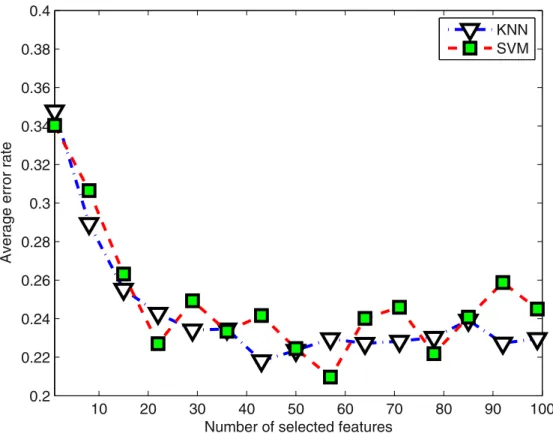
Figure 2 shows how classification performance varies with the change in number of features which were selected. The average classification error rate was calculated by two classifiers on all test datasets. An improvement in performance could be evident if the number of related features increase from 1 to 25, but after increasing number of features beyond 25, no significant improve-ment was obvious. In order to find optimum results for all the datasets, we extend the range from 20 to 50 features configurations in our study.
Results
Test datasets
To assess the performance of our method, we have conducted several experiments on a number of publicly available datasets. Summary of all data sets we used in our experiments can be found in table 2 and following is the brief description of each data set.
N
AMLALL(A)([27]). There are two parts containing the initial (train), 38 bone marrow samples from two classes: 27 cases of acute lymhoblastic leukemia(ALL) and 11 cases of acute myeloid leukemia(AML); independent (test), 34 samples from two classes: 20 cases of ALL and 14 cases of AML. Each case is described by expression levels of 7129 probes from 6817 Figure 1. The geometric representation of PLS and kernel PLS.(a) In the original space, the componentstl,l[f1,2gare on planer. (b) We projected the data into the kernel space by mappingW(:)and the componentstWare captured in kernel space. The weight of each feature is estimated byarg minvl~EtW
l{xivlE,i[f1,2, ,Ng. doi:10.1371/journal.pone.0102541.g001
Table 1.Algorithm 1: kernelPLS.
Input:KX – kernel matrix
KY– kernel matrix
Output:w– the weight of each feature 1: InitializingK1/KX,c1~z?;
e~0:01,l~1;
2:whileclwec1do
3: Initializing the projection directionbW 0,b
W
l; 4: whileEbWl{b
W 0Ew do
5: bW0/b W
l; 6: bW
l/KYKlb
W
l;
7: bWl/ bW
l
EbW
lE
;
8: end while
9: Calculating the componenttW
l,t
W
l/KlbWl;
10: Deflating target matrixYl,Ylz1/Yl{D{1tW
lt
W
l
T
Yl, whereD~tW
l
T
tW
l; 11: Deflating kernel matrixKl,Klz1/(I{D{1
tW
lt
W
l
T
)Kl(I{D {1 tW lt W l T );
12: Calculating the contribution of thelth componentcl,cl~
XM
i~1Nim W
il
XM
i~1Ni
;
13: l~lz1;
14:end while
15:h~l{1
16: Calculating the weight of each featurewvia Equation(1)
17:returnw
doi:10.1371/journal.pone.0102541.t001
arg maxa[ N
ϵ
R
human genes. Source: http://www-genome.wi.mit.edu/ cgi-bin/cancer/datasets.cgi;
N
Breast(B)([28]). The dataset used the raw intensity Affym-etrix CEL files and normalized the data by RMA procedures. A final expression matrix comprising 22283 features and 209 samples, 71 of which are from patients, the rest 138 samples are normal samples. Source: http://math.bu.edu/people/ sray/software/prediction;N
Lung(L)([29]). This dataset contains 86 samples: 24 are tumor samples and 62 are normal controls, 7129 genes with highest intensity across the samples are considered. Source: http://math.bu.edu/people/sray/software/prediction/;N
Prostate(P) ([30]).This dataset contains 52 prostate tumor samples and 50 normal samples with 12600 genes. An independent set of testing samples is generated from the training data, 25 tumor and 9 normal samples are extracted Figure 2. The effect of different numbers of selected features. Two classifier, SVM and KNN, are used for measuring the performance of average error of all test datasets based on kernelPLS selector. Where the optimal parameters of RBF kernel SVM are determined by partial swarm optimization and the parameterkfor the nearest neighbors is 5.doi:10.1371/journal.pone.0102541.g002
Table 2.The cancer classification datasets1used in the present paper.
Class Dataset Sample Feature Class Source
AMLALL 72 7129 2 [27]
Breast 209 22283 2 [42]
Two-class
Lung 86 7129 2 [29]
Prostate 102 12600 2 [30]
DLBCL 77 7129 2 [31]
Medulloblastoma 60 7129 2 [32]
Stjude 215 12558 7 [13]
Lymphoma 62 4026 3 [33]
Multi-class
SRBCT 83 2308 4 [34]
MLL 72 8685 3 [35]
Lung 203 3312 5 [37]
1Available at https://github.com/sqsun/kernelPLS-datasets.
according to Singh’s publication. Source (training): http:// www.broadinstitute.org/cgi-bin/cancer/datasets.cgi;
N
DLBCL(D)([31]). The goal of this dataset is to distinguish diffuse large B-cell lymphoma (DLBCL) from follicular lymphoma (FL) morphology. This dataset contains 58 DLBCL samples and 19 FL samples. The expression profile contains 7129 genes. Source: http://www-genome.wi.mit.edu/mpr/ prostate;N
Medulloblastoma(M)([32]). Patients outcome prediction for central nervous system embryonal tumor. Survivors are patients who are alive after treatment whiles the failures are those who succumbed to their disease. The dataset contains 60 patient samples, 21 are survivors and 39 are failures. There are 7129 genes in the dataset. Source: http://www-genome.wi. mit.edu/mpr/CNS;N
Stjude(S)([13]). The dataset has been divided into six diagnostic groups, BCR-ABL (9 samples), E2A-PBX1 (18 samples), Hyperdiploidw50 (42 samples), MLL (14 samples),T-ALL (28 samples) and TEL-AML1 (52 samples)), and one that contains diagnostic samples (52 samples) that did not fit into any one of the above groups. There are 12558 genes. Source: http://www.stjuderesearch.org/data/ALL1;
N
Lymphoma(Ly)([33]). The dataset consists of measure-ments of 4026 genes from 62 patients. The patients are classified into three classes: lymphoma and leukemia (DLCL, 42 samples), follicular lymphoma (FL, 9 samples) and chronic lymphocytic leukemia (CLL, 11 samples). We estimated the missing values of ‘‘NA’’ symbol in original ratio data by KNN-imputed method (k~10). Source: http://llmpp.nih.gov/ lymphoma;N
SRBCT(SR)([34]). The dataset contains 83 samples and 2,308 gene expression values. It can be divided into four classes, the Ewing family of tumors (EWS), Burkitt lymphoma(BL), neuroblastoma (NB) and rhabdomyosarcoma (RMS). Among the 83 samples, 29, 11, 18, and 25 samples belong to classesEWS, BL, NB and RMS, respectively. Source: http://www. biomedcentral.com/content/supplementary/1471-2105-7-228-S4.tgz.
N
MLL(ML)([35]). The dataset contains 72 samples in three classes, acute lymphoblastic leukemia (ALL), acute myeloid leukemia (AML), and mixed-lineage leukemia gene (MLL), which have 24, 28, 20 samples, respectively. In our experiment, we preprocessed this dataset according to reference [36] and obtained a dataset with 72 samples and 8685 genes. Source: http://www.biomedcentral.com/ con-tent/supplementary/1471-2105-7-228-S4.tgz.N
Lung(Lu)([37]).The total of this dataset contains 203 samples with 12600 genes in five classes, adenocarcinomas (139), squamous cell lung carcinomas (21), pulmonary carcinoids (20), small-cell lung carcinomas(6) and normal lung (17). We preprocessed the dataset according to reference [36] and obtained a dataset with 203 samples and 3312 genes. Source: http://www.biomedcentral.com/content/supplementary/ 1471-2105-7-228-S4.tgz.Comparison of selected genes
In our first experiment, we used two datasets, namely the Leukemia data (two-class) of [27] and the Lymphoma data(three-class) of [33], to compare our method with previous works with respect to the selected genes.
For the Leukemia data, we collected several most important genes (in table 3) that were published in several papers. It can readily be seen that three probes, X95735_at, M27891_at and M23197_at were reported by five published papers, and their ranking by our method are 4th, 17st and 8st, respectively. We notice that there are many overlapping of genes among the list of papers.
For Leukemia data, the top-ranked 40 features obtained by our procedure are shown in table 4 in which genes are in columns from 1 to 40. There is a worthwhile result achieved by our
Table 3.Description of genes reported by existing published papers and ranked by our method.
Accession number Gene description References Rank
X95735_at Zyxin [43] [38] [27] [44] [28] 4
M23197_at CD33 [43] [38] [27] [44] [28] 8
U22376_cds2_s_at C-myb [38] [27] [44] [28] 74
M27891_at Cystatin C [43] [38] [27] [44] [28] 21
M16038_at LYN [38] [27] [44] [28] 11
M84526_at DF(adipsin) [43] [38] [27] [44] 9
M27783_s_at ELA2 Elastatse 2 [38] [44] [28] 80
U50136_rna1_at LTC4 synthase [38] [27] [28] 3
Y12670_at Leptin receptor [38] [27] [28] 2
U46499_at Glutathione [43] [38] [44] 96
L09209_s_at Amyloid beta [43] [38] [44] 48
U46751_at p62 [38] [27] 19
M55150_at Fumarylacetoacetate [38] [27] 7
M83652_s_at Properdin [38] [27] 22
M80254_at CyP3 [27] [28] 17
X17042_at Proteoglycan 1 [43] [27] 10
U82759_at HoxA9 [43] [27] 8
method, that is, it obtained the genes with the highest weight. Many of these genes are known as differentially expressed genes by many foregoing studies. 24 out of 40 genes are listed in this table that were also selected by [27], which shows the effectiveness of our method.
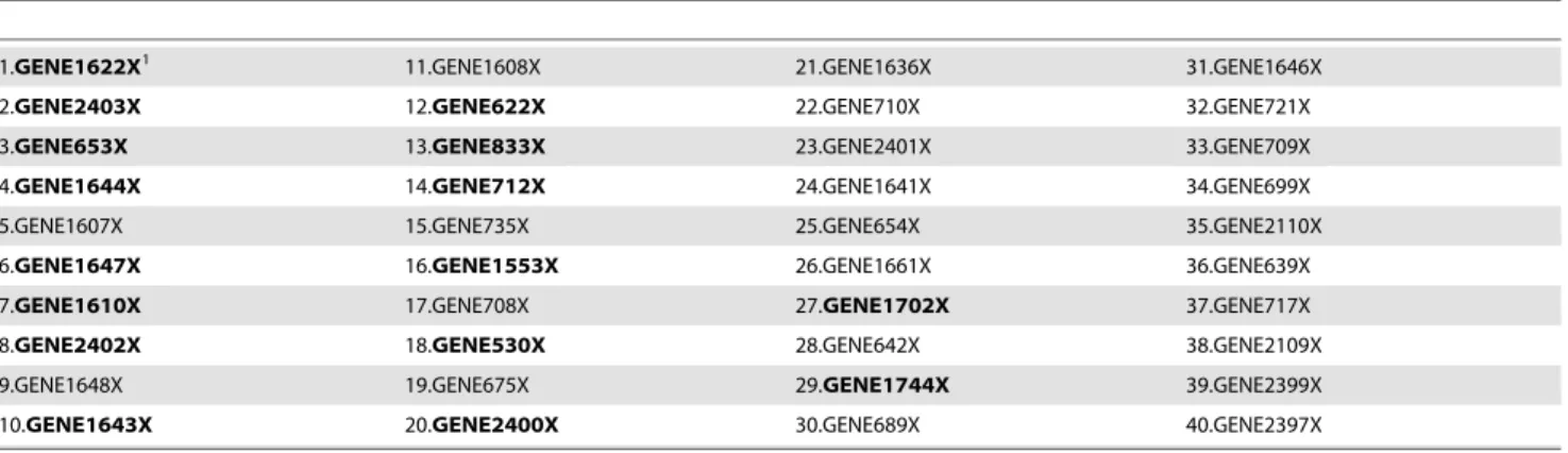
For the Lymphoma data of [33], the missing values are imputed by KNN-imputed method(k~10). The top 40 genes ranked by our procedure are listed in table 5. From the table, We can see that important genes can be captured easily by our method. There are many genes that are also chosen by [38].
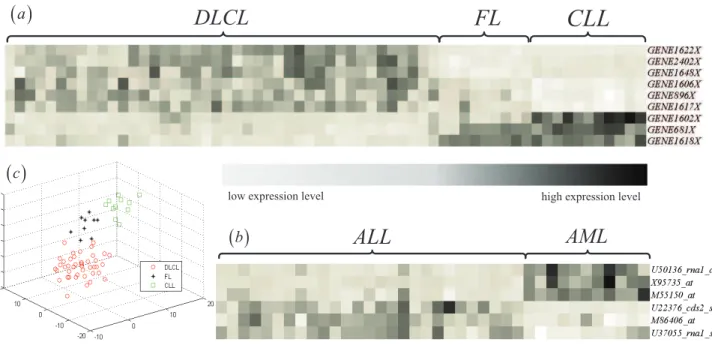
Figure 3 illustrates the differentially expressed genes for two datasets, namely the Leukemia data and the Lymphoma data. No single gene is uniformly expressed across the class, all these genes as a group appear correlated with class which is illustrating the effectiveness of the Kernel PLS method. In Figure 3(a) the top panel is consist of three genes GENE1622X, GENE2402X and GENE1648X that are highly expressed in DLCL, middle panel is comprised of GENE1606X, GENE896X and GENE1617X that are highly expressed in DLCL but moderately expressed in FL. Bottom panel compose of three genes, namely GENE1602X,-GENE681X and GENE1618X, are more highly expressed in CLL. In Figure 3(b) the top panel shows three probes highly express in AML and the bottom panel shows three probes more highly expression in ALL. The probe U377055_rna1_s_at was found by our method to distinguish AML from ALL. Figure 3(c) demonstrate the projected result of top 100 genes using sammon
mapping which shows DLBCL, CLL, FL are very clear and the boundaries can be easily drawn.
Comparison of several multivariate-based feature selectors
In our second experiment, we compared several feature selectors with our procedure based on two classifiers, SVM and KNN. In our experiments, we choose the RBF kernel for each dataset to perform classification. To determine the best values of C(-c) and c(-g), we conducted particle swarm optimization algorithm to pick the pair (C,c) with best accuracy in the range ofC[f10{3, ,102gandc[f10{3, ,104g. We set the param-eter to k~5 for k-nearest neighbor. To obtain a statistically reliable predictive measurement, we performed 10-fold cross validation for two-class datasets and 5-fold cross validation for multi-class datasets. The results are evaluated by classification accuracy(Acc), area under receiver operating characteristic curve (AUC) for two-class problems and classification accuracy(Acc), Cohen’s Kappa coefficient(Kappa) for multi-class problems. The reason of using 5-fold cross validation for multi-class datasets is that there is just a few number of samples in some groups (classes) of these datasets. Therefore to ensure the presence of samples of each class in training and also in test datasets we need to perform 5-fold cross validation for multi-class datasets.
In this paper, the comparison was conducted with four competitive algorithms, PLS, ReliefF, SVMrfe and mRMR. The
Table 4.Top-ranked 40 features selected using kernelPLS for the Leukemia dataset.
1.M23197_at1 11.M16038_at 21.M27891_at 31.M28130_rna1_s_at
2.Y12670_at 12.M96326_rna1_at 22.M83652_s_at 32.M37435_at
3.U50136_rna1_at 13.X70297_at 23.M19507_at 33.M98399_s_at
4.X95735_at 14.M62762_at 24.M63138_at 34.U12471_cds1_at
5.D49950_at 15.X85116_rna1_s_at 25.X58431_rna2_s_at 35.U37055_rna1_s_at
6.X04085_rna1_at 16.L08246_at 26.Y00787_s_at 36.U67963_at
7.M55150_at 17.M80254_at 27.M68891_at 37.Y07604_at
8.U82759_at 18.M22960_at 28.X52056_at 38.M69043_at
9.M84526_at 19.U46751_at 29.M11147_at 39.U63289_at
10.X17042_at 20.M81933_at 30.M57710_at 40.M81695_s_at
1The boldfaced probes were selected by [27].
doi:10.1371/journal.pone.0102541.t004
Table 5.Top-ranked 40 features selected using kernelPLS for the Lymphoma dataset.
1.GENE1622X1 11.GENE1608X 21.GENE1636X 31.GENE1646X
2.GENE2403X 12.GENE622X 22.GENE710X 32.GENE721X
3.GENE653X 13.GENE833X 23.GENE2401X 33.GENE709X
4.GENE1644X 14.GENE712X 24.GENE1641X 34.GENE699X
5.GENE1607X 15.GENE735X 25.GENE654X 35.GENE2110X
6.GENE1647X 16.GENE1553X 26.GENE1661X 36.GENE639X
7.GENE1610X 17.GENE708X 27.GENE1702X 37.GENE717X
8.GENE2402X 18.GENE530X 28.GENE642X 38.GENE2109X
9.GENE1648X 19.GENE675X 29.GENE1744X 39.GENE2399X
10.GENE1643X 20.GENE2400X 30.GENE689X 40.GENE2397X
1The boldfaced genes were selected by [38].
parameter setting of them are as follows: for the PLS-based feature selection, we used the SIMPLS method and the number of components determined by self-adaptive manner which is the same as the kernelPLS (the proposed method). The parameterkof ReliefF is equal to the number of sample according to the published paper [39]. For SVMrfe, in order to ensure acceptable running time, we use SVM with RBF kernel and its parameter settings are same as in LIBSVM.
Without loss of generality, we used two datasets, Breast(two-class) and Lymphoma(three-Breast(two-class) to show the performance of our method. Figure 4 shows the comparison of error rate between our method and four other methods. One can see that when number of selected features are 30, error rate of our method is less than other methods for both classifiers and both datasets.
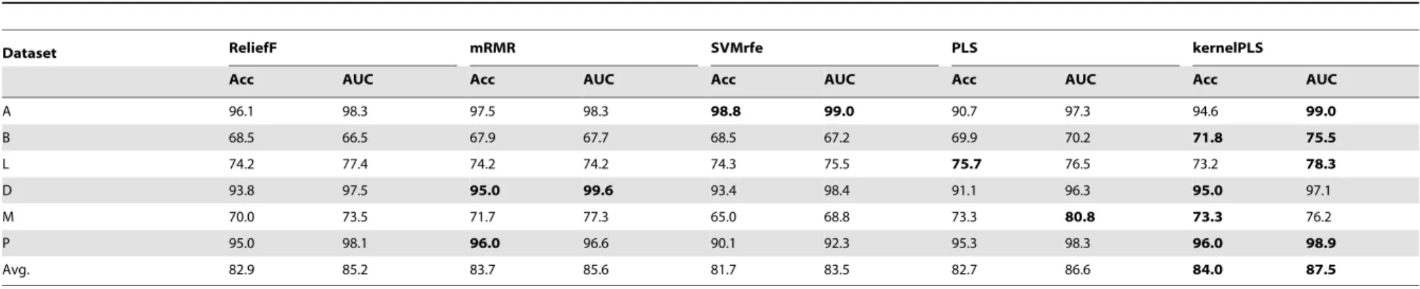
Table 6 and 7 summarized the comparison of results generated by our method and other methods with respect to Acc and AUC for two-class datasets. From the results, we can see that the performance of our method is better than others. Refers to table 6 we can see that for Breast(B) and Prostate(P) datasets, accuracy of our method is considerably higher as compare to other methods, which shows the effectiveness of our method.
Similarly in table 7 for datasets Breast, Lung, DLBCL, Medulloblastoma, Prostate and Stjude, kernelPLS shown better accuracy rate for SVM classifier wrather than KNN. Both Acc and AUC values of our method have higher values among others and finally the average results likewise are best. Although for few datasets our results are similar to their results but in these cases time taken by our method is significantly smaller than other methods. For example in table 7 for AMLALL dataset, including our method, the AUC is 100% for many methods but time consumed by our method is only 0.0891 s while the time taken by other methods, ReliefF, mRMR, SVMrfe and PLS, are about 5 s, 52 s, 210 s and 12 s, respectively. So time consumption by our
algorithm is many times less than others which depicts overall well performance of our method.
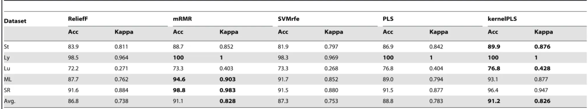
It is worth noting that our method outperforms others on three hard-classify datasets, Wang’s Breast cancer, Gordon’s Lung adenocarcinoma and Pomeroy’s Medulloblastoma. We also make a comparison with the results of other feature selectors in published papers. Fox example, the reference [40] reported that the accuracies of k-TSP+SVM on these datasets were 67.1%, 72.2% and 64.2%, respectively. The reference [41] combined multiple feature selection (or feature transform) approaches for Medulloblastoma dataset and the obtained highest Acc was 70%. To estimate the performance of our method we did not limit our evaluation to only two-class datasets we also used 5 multi-class datasets in our experiments. Tables 8 and 9 demonstrate the comparison of kernelPLS with other methods for multi-class datasets on the bases of results obtained for two evaluation measures, namely Acc and Kappa. Results shown in table 8 and table 9 are for two classifiers KNN and SVM, respectively. In table 8 results obtained by kernelPLS are better than Relief, SVMrfe and PLS and highly competitive to mRMR method for several multi-class datasets. For example in case of Stjude dataset for Acc and Kappa values by kernelPLS are 96.4% and 0.956 respectively which are highest among all values achieved by other methods. Likewise table 9 authenticates the high performance by kernelPLS over other methods for SVM classifier. Here one can see that kernelPLS give outperforming results for all datasets by achieving accuracies and Kappa coefficients values superior than all other methods. As a conclusion the overall high average Acc and Kappa values in both tables show the effectiveness and significance of our method as compare to other popular methods. Table 10 shows the comparison between running time taken by our method and other methods. There is no single method among these that can perform faster than our method. It clearly shows that kernelPLS is faster than the other algorithms. For example for
Figure 3. The genes expression levels of two datasets, namely the Leukemia and the Lymphoma data. Expression levels for each gene are normalized across the samples such that the mean is 0 and the SD is 1. Expression levels greater than the mean are shaded in black, and those below the mean are shaded in white. (a) The expression profiles of the Lymphoma dataset. Each row corresponds to a gene, with the columns corresponding to expression levels in different samples. (b) The expression profiles of the Leukemia dataset. Each row expresses a probe while each column describes expression level in different samples. (c) Display the results on the Lymphoma dataset using sammon mapping. This projection expresses the gene expression levels of genes that perfectly separate the three types of Lymphoma subtypes, i.e. DLBCL, FL, and CLL.
AMLALL dataset time consumed by our method is 0.0891 s while time spent by ReliefF, mRMR, SVMrfe and PLS are 5.1510 s, 52.5854 s, 210.4046 s, 12.1222 s, respectively.
Discussion
In this article, we proposed an effective multivariate-based feature filter method for cancer classification, namely, kernelPLS-based filter method. We showed that gene-gene interactions cannot be ignored in feature selection techniques to improve classification performance. In other words the nonlinear relation-ship of gene-gene interactions is a vital concept that can be taken into account to enhance accuracy. To capture these nonlinear relations of interaction between genes we used kernel method because kernel method can be used to reveal the intrinsic relationships that are hidden in the raw data. In order to capture the reasonable number of components, we make use of the relationship between PLS and linear discriminant analysis to determine the number of components in kernel space based on kernel linear discriminant analysis. To verify the importance of gene-gene interactions we compared our feature selector with other multivariate-based feature selection methods by using two
classifiers SVM and KNN. Experimental results, expressed as both accuracy(Acc) and area under the ROC curve(AUC), showed that our method leads to promising improvement in ACC and AUC. We can conclude that the gene-gene interactions whats more, nonlinear relationships of gene-gene interactions are core interactions that can improve classification accuracy, efficiently. We can summarize the characteristics of proposed approach as follows: (1)Fast and efficient. The time complexity of deflation procedure used after the extraction of each component scale is
O(N2), where N is the number of sample. In most cases, the number of sample in microarray data is less than 150, therefore, the running speed of kernelPLS procedure(feature selection time) is faster than others, which are summarized in table 10. (2)Model-free, e.g. no need the distributional assumptions. Because of small sample size, it is difficult to validate distributional assumptions, such as Gaussian distribution, Gamma distribution etc. (3)Appli-cable to both two-class as well as multi-class classification problems.
In our method, the choice of kernel functions can affect the results. When high dimensionality exist(such as microarray datasets), the performance of linear kernel is better than Gauss
Figure 4. Classification error rate of different number of selected features using two classifiers, KNN and SVM. (a) and (b) indicate the results on the Breast dataset. (c) and (d) indicate the results on the Lymphoma dataset.
Dataset ReliefF mRMR SVMrfe PLS kernelPLS
Acc AUC Acc AUC Acc AUC Acc AUC Acc AUC
A 96.1 98.3 97.5 98.3 98.8 99.0 90.7 97.3 94.6 99.0
B 68.5 66.5 67.9 67.7 68.5 67.2 69.9 70.2 71.8 75.5
L 74.2 77.4 74.2 74.2 74.3 75.5 75.7 76.5 73.2 78.3
D 93.8 97.5 95.0 99.6 93.4 98.4 91.1 96.3 95.0 97.1
M 70.0 73.5 71.7 77.3 65.0 68.8 73.3 80.8 73.3 76.2
P 95.0 98.1 96.0 96.6 90.1 92.3 95.3 98.3 96.0 98.9
Avg. 82.9 85.2 83.7 85.6 81.7 83.5 82.7 86.6 84.0 87.5
doi:10.1371/journal.pone.0102541.t006
Table 7.Comparison of kernelPLS with four other methods. For 10-fold cross validation classification accuracy(%) and AUC (%) of SVM on two-class datasets.
Dataset ReliefF mRMR SVMrfe PLS kernelPLS
Acc AUC Acc AUC Acc AUC Acc AUC Acc AUC
A 97.5 100 96.3 100 97.5 100 94.6 100 96.1 100
B 68.0 69.2 69.9 67.5 69.9 69.7 72.2 71.5 72.7 75.4
L 77.4 81.5 72.1 76.5 73.3 75.8 76.8 77.6 77.4 82.6
D 94.8 99.2 94.8 99.2 93.4 99.4 93.4 98.3 97.5 100
M 71.7 72.9 70 73.1 66.7 69.7 70 77.2 73.3 82.7
P 96.0 97.5 96.0 96.7 89.1 94.2 95.1 98.7 97.3 97.9
Avg. 84.2 86.7 83.2 85.5 81.7 84.8 83.7 87.2 85.7 89.8
doi:10.1371/journal.pone.0102541.t007
A
Kernel-Based
Multivariat
e
Feature
Selection
Method
ONE
|
www.ploson
e.org
9
July
2014
|
Volume
9
|
Issue
7
|
Dataset ReliefF mRMR SVMrfe PLS kernelPLS
Acc Kappa Acc Kappa Acc Kappa Acc Kappa Acc Kappa
St 83.9 0.811 88.7 0.852 81.9 0.797 86.9 0.842 89.9 0.876
Ly 98.5 0.964 100 1 98.3 0.969 100 1 100 1
Lu 72.2 0.271 73.3 0.403 73.3 0.268 76.8 0.404 76.8 0.428
ML 87.7 0.762 94.6 0.903 91.7 0.852 89.0 0.794 93.1 0.877
SR 91.6 0.884 98.8 0.983 91.5 0.880 91.5 0.877 96.4 0.947
Avg. 86.8 0.738 91.1 0.828 87.3 0.753 88.8 0.783 91.2 0.826
doi:10.1371/journal.pone.0102541.t008
Table 9.Comparison of kernelPLS with four other methods. For 5-fold cross validation classification accuracy(%) and Cohen’s kappa coefficient of SVM on multi-class datasets.
Dataset ReliefF mRMR SVMrfe PLS kernelPLS
Acc Kappa Acc Kappa Acc Kappa Acc Kappa Acc Kappa
St 86.2 0.849 88.9 0.866 86.4 0.851 86.8 0.834 89.9 0.876
Ly 100 1 100 1 96.7 0.933 100 1 100 1
Lu 76.9 0.451 76.9 0.399 74.6 0.382 74.5 0.360 79.2 0.532
ML 94.6 0.906 93.2 0.884 87.7 0.801 90.3 0.834 95.8 0.919
SR 96.4 0.947 98.8 0.983 97.6 0.964 98.8 0.983 97.6 0.964
Avg. 90.8 0.831 91.6 0.826 88.6 0.786 90.1 0.802 92.5 0.858
doi:10.1371/journal.pone.0102541.t009
A
Kernel-Based
Multivariat
e
Feature
Selection
Method
ONE
|
www.ploson
e.org
10
July
2014
|
Volume
9
|
Issue
7
|
kernel for our method. What’s more, in case of linear kernel there is no noticeable effect on the results while adjusting its parameters.
Author Contributions
Conceived and designed the experiments: SS QP. Performed the experiments: SS. Analyzed the data: SS AS. Contributed reagents/ materials/analysis tools: SS. Contributed to the writing of the manuscript: SS AS.
References
1. Piao Y, Piao M, Park K, Ryu KH (2012) An ensemble correlation-based gene selection algorithm for cancer classification with gene expression data. Bioinformatics 28: 3306–3315.
2. Kohavi R, John GH (1997) Wrappers for feature subset selection. Artificial Intelligence 97: 273–324.
3. Xiong M, Fang X, Zhao J (2001) Biomarker identification by feature wrappers. Genome Research 11: 1878–1887.
4. Senthamarai Kannan S, Ramaraj N (2010) A novel hybrid feature selection via symmetrical uncertainty ranking based local memetic search algorithm. Knowledge-Based Systems 23: 580–585.
5. Dı´az-Uriarte R, Andre´s SAd (2006) Gene selection and classification of microarray data using random forest. BMC Bioinformatics 7.
6. Lei Y, Huan L (2004) Efficient feature selection via analysis of relevance and redundancy. Journal of Machine Learning Research 5: 1205–1224. 7. Peng H, Fulmi L, Ding C (2005) Feature selection based on mutual information
criteria of maxdependency, max-relevance, and min-redundancy. IEEE Transactions on Pattern Analysis and Machine Intelligence 27: 1226–1238. 8. Saeys Y, Inza I, Larranaga P (2007) A review of feature selection techniques in
bioinformatics. Bioinformatics 23: 2507–2517.
9. Gavin B, Adam P, Ming-Jie Z, Mikel L (2012) Conditional likelihood maximisation: a unifying framework for information theoretic feature selection. Journal of Machine Learning Research 13: 27–66.
10. Isabelle G, Andr Elisseeff (2003) An introduction to variable and feature selection. The Journal of Machine Learning Research 3: 1157–1182. 11. Balagani KS, Phoha VV (2010) On the feature selection criterion based on an
approximation of multidimensional mutual information. IEEE Transactions on Pattern Analysis and Machine Intelligence 32: 1342–1343.
12. De Jay N, Papillon-Cavanagh S, Olsen C, El-Hachem N, Bontempi G, et al. (2013) mrmre: an r package for parallelized mrmr ensemble feature selection. Bioinformatics 29: 2365–2368.
13. Yeoh EJ, Ross ME, Shurtleff SA, Williams WK, Patel D, et al. (2002) Classification, subtype discovery, and prediction of outcome in pediatric acute lymphoblastic leukemia by gene expression profiling. Cancer Cell 1: 133–143. 14. Gevaert O, Smet FD, Timmerman D, Moreau Y, Moor BD (2006) Predicting
the prognosis of breast cancer by integrating clinical and microarray data with bayesian networks. Bioinformatics 22: e184–e190.
15. Sun X, Liu Y, Li J, Zhu J, Chen H, et al. (2012) Feature evaluation and selection with cooperative game theory. Pattern Recognition 45: 2992–3002. 16. Wold S, Ruhe A, Wold H, Dunn IW (1984) The collinearity problem in linear
regression. the partial least squares (pls) approach to generalized inverses. SIAM Journal of Scientific and Statistical Computations 5: 735-743.
17. Gutkin M, Shamir R, Dror G (2009) Slimpls: a method for feature selection in gene expression-based disease classification. Plos One 4.
18. You W, Yang Z, Ji G (2014) Pls-based recursive feature elimination for high-dimensional small sample. Knowledge-Based Systems 55: 15–28.
19. You W, Yang Z, Ji G (2014) Feature selection for high-dimensional multi-category data using pls-based local recursive feature elimination. Expert Systems with Applications 41: 1463–1475.
20. You W, Yang Z, Yuan M, Ji G (2014) Totalpls: Local dimension reduction for multicategory microarray data. IEEE Transactions on Human-Machine Systems 44: 125–138.
21. Wold H (1966) Estimation of principal components and related models by iterative least squares. Multivariate Analysis. New York: Academic.
22. Shawe-Taylor J, Nello C (2004) Kernel methods for pattern analysis. UK: Cambridge University.
23. Ra´nnar S, Lindgren F, Geladi P, Wold S (1994) A pls kernel algorithm for data sets with many variables and fewer objects. part 1: Theory and algorithm. Journal of Chemometrics 8: 111–125.
24. Wold S, Johansson W, Cocchi M (1993) PLS-partial least-squares projections to latent structures. 3D QSAR in Drug Design, Theory Methods and Applications. Berlin: Springer-Verlag.
25. Ji G, Yang Z, You W (2011) Pls-based gene selection and identification of tumor-specific genes. IEEE Transactions on Systems Man and Cybernetics Part C-Applications and Reviews 41: 830–841.
26. Li GZ, Zhao RW, Qu HN, You M (2012) Model selection for partial least squares based dimension reduction. Pattern Recognition Letters 33: 524–529. 27. Golub TR, Slonim DK, Tamayo P, Huard C, Gaasenbeek M, et al. (1999)
Molecular classification of cancer: class discovery and class prediction by gene expression monitoring. Science 286: 531–537.
28. Wang HQ, Wong HS, Huang DS, Shu J (2007) Extracting gene regulation information for cancer classification. Pattern Recognition 40: 3379–3392. 29. Gordon GJ, Jensen RV, Hsiao LL, Gullans SR, Blumenstock JE, et al. (2002)
Translation of microarray data into clinically relevant cancer diagnostic tests using gene expression ratios in lung cancer and mesothelioma. Cancer Research 62: 4963–4967.
30. Singh D, Febbo PG, Ross K, Jackson DG, Manola J, et al. (2002) Gene expression correlates of clinical prostate cancer behavior. Cancer Cell 1: 203– 209.
31. Shipp MA, Ross KN, Tamayo P, Weng AP, Kutok JL, et al. (2002) Diffuse large b-cell lymphoma outcome prediction by gene-expression profiling and supervised machine learning. Nature Medicine 8: 68–74.
32. Pomeroy SL, Tamayo P, Gaasenbeek M, Sturla LM, Angelo M, et al. (2002) Prediction of central nervous system embryonal tumour outcome based on gene expression. Nature 415: 436–442.
33. Alizadeh AA, Eisen MB, Davis RE, Ma C, Lossos IS, et al. (2000) Distinct types of diffuse large b-cell lymphoma identified by gene expression profiling. Nature 403: 503–511.
34. Khan J, Wei JS, Ringner M, Saal LH, Ladanyi M, et al. (2001) Classification and diagnostic prediction of cancers using gene expression profiling and artificial neural networks. Nature Medicine 7: 673–679.
Table 10.The running time(s) of five feature filtering methods on two groups cancer classification datasets.
Class Dataset ReliefF mRMR1 SVMrfe PLS kernelPLS
A 5.1510 52.5854 210.4046 12.1222 0.0891
B 5.1496 88.6176 w1e+003 10.6423 0.1092
Two-class
L 7.5420 52.8977 693.1857 16.8629 0.2410
D 5.5614 53.1088 221.2261 12.0526 0.0965
M 5.1343 51.9969 421.8250 19.2384 0.2676
P 18.1848 65.1076 w1e+003 64.2148 0.6010
St 34.0030 67.5321 w1e+003 w1e+003 2.1180
Ly 2.7332 5.7846 217.2568 27.9456 0.2361
Multi-class
Lu 10.2526 9.7816 w1e+003 17.8940 0.5500
ML 6.6426 8.7484 791.0244 98.8890 0.2586
SR 1.8230 5.8336 87.6536 8.8784 0.1714
1Time required for selecting 1000 features.
35. Armstrong SA, Staunton JE, Silverman LB, Pieters R, de Boer ML, et al. (2002) Mll translocations specify a distinct gene expression profile that distinguishes a unique leukemia. Nature Genetics 30: 41–47.
36. Yang K, Cai ZP, Li JZ, Lin GH (2006) A stable gene selection in microarray data analysis. BMC Bioinformatics 7.
37. Bhattacharjee A, Richards WG, Staunton J, Li C, Monti S, et al. (2001) Classification of human lung carcinomas by mrna expression profiling reveals distinct adenocarcinoma subclasses. Proceedings Of the National Academy Of Sciences Of the United States Of America 98: 13790–13795.
38. Dramiski M, Rada-Iglesias A, Enroth S, Wadelius C, Koronacki J, et al. (2008) Monte carlo feature selection for supervised classification. Bioinformatics 24: 110–117.
39. Brown G, Pocock A, Zhao MJ, Lujn M (2012) Conditional likelihood maximisation: a unifying framework for information theoretic feature selection. The Journal of Machine Learning Research 13: 27–66.
40. Shi P, Ray S, Zhu Q, Kon MA (2011) Top scoring pairs for feature selection in machine learning and applications to cancer outcome prediction. Bmc Bioinformatics 12.
41. Nanni L, Brahnam S, Lumini A (2012) Combining multiple approaches for gene microarray classification. Bioinformatics 28: 1151–1157.
42. Wang Y, Klijn JGM, Zhang Y, Sieuwerts AM, Look MP, et al. (2005) Gene-expression profiles to predict distant metastasis of lymph-node-negative primary breast cancer. The Lancet 365: 671–679.
43. Chu W, Ghahramani Z, Falciani F, Wild DL (2005) Biomarker discovery in microarray gene expression data with gaussian processes. Bioinformatics 21: 3385–3393.