Digital elevation model quality on digital soil mapping prediction accuracy

In this context, the main objective of this research was to assess the use of DSM techniques for mapping soils in western Haiti, specifically by assessing the importance

ma-se como um organismo que, quer a montante quer a jusante, articula com os mais diversos ser- viços: Centros de Emprego, Centros de Forma- ção Profissional, Serviços de

The objective of this study was to predict the levels of organic carbon (OC), clay, and extractable phosphorus (P), from the spectral responses of soil samples in the visible and

This study aimed to determine equations to estimate soil moisture using variables of color spaces obtained from images of a portable digital camera.. Material

The aim of this study was to map local soil classes by computer-assisted cartography (CAC), using several combinations of topographic properties produced by GIS (digital

In this context, this study differs from previous work in its objective to compare the efficiency of the two prediction methods (ANNs and MLC) for digital soil mapping, using

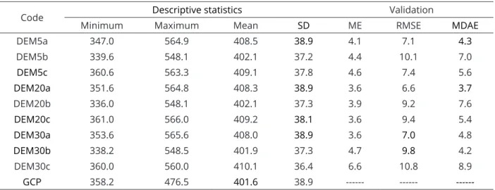
precision elevation by statistical tests based on field reference points, the root mean square error (RMSE), identification of the number and size of spurious depressions, and

There is no straightforward decision on whether to use ordinary kriging or regression kriging for mapping soil properties, because the quality of predictions depends on

REFERENCES

AGRESTI, A. Categorical data analysis. New York John Wiley Sons. Gainesville, 2002. 710p.
ALVARES, C. A. et al. Koppen’s climate classification map for Brazil. Meteorologische Zeitschrift, 22(6):711-728, 2014.
ANTUNES, M. A. H.; DEBIASI, P.; SIQUEIRA, J. C. DOS S. Avaliação
espectral e geométrica das imagens Rapideye e seu potencial
para o mapeamento e monitoramento agrícola e ambiental.
Revista Brasileira de Cartografia, 66(1):105-113, 2014.
BALTENSWEILER, A. et al. Terrestrial laser scanning improves
digital elevation models and topsoil pH modelling in
regions with complex topography and dense vegetation. Environmental Modelling and Software, 95(1):13-21, 2017.
BEHRENS, T. et al. Multi-scale digital terrain analysis and feature
selection for digital soil mapping. Geoderma, 155(3-4):175-185, 2010.
BEHRENS, T. et al. Hyper-scale digital soil mapping and soil
formation analysis. Geoderma, 213:578-588, 2014.
CAVAZZI, S. et al. Are fine resolution digital elevation models always the best choice in digital soil mapping? Geoderma,
195(196):111-121, 2013.
CHAGAS, C. S. et al. Avaliação de modelos digitais de elevação para aplicação em um mapeamento digital de solos.
Revista Brasileira de Engenharia Agrícola e Ambiental,
14(21):218-226, 2010.
FAN., L.; ATKINSON, P. M. Accuracy of digital elevation models
derived from terrestrial laser scanning Data. Geoscience and Remote Sensing Letters, IEEE, 12(9):1923-1927, 2015.
FISHER, P. F.; TATE, N. J. Causes and consequences of error in
digital elevation models. Progress in Physical Geography,
30(4):467-489, 2006.
FLORINSKY, I. V. Accuracy of local topographic variables derived
from digital elevation models. International Journal of Geographical Information Science, 12(1):47-61, 1998.
HENGL, T. et al. SoilGrids250m: Global gridded soil information
based on machine learning. PLOS ONE, 12(2):1-40, 2017.
HENGL, T.; GRUBER, S.; SHESTHA, D. P. Reduction of errors in
digital terrain parameters used in soil-landscape modelling.
International Journal of Applied Earth Observation and Geoinformation,5:97-112 , 2004.
HEUNG, B. et al. An overview and comparison of machine-learning techniques for classification purposes in digital
soil mapping. Geoderma, 265:62-77, 2016.
HIRT, C.; FILMER, M. S.; FEATHERSTONE, W. E. Comparison and
validation of the recent freely available ASTER-GDEM ver1,
SRTM ver4.1 and GEODATA DEM-9S ver3 digital elevation
models over Australia. Australian Journal of Earth Sciences, 57(3):337-347, 2010.
HÖHLE, J.; HÖHLE, M. Accuracy assessment of digital elevation
models by means of robust statistical methods. ISPRS Journal of Photogrammetry and Remote Sensing, 64(4): 398-406, 2009.
HUTCHINSON, M. F. A new procedure for gridding elevation and streamline data with automatic removal of spurious
pits. Journal of Hydrology, 106:211-232, 1989.
MAYNARD, J. J.; JOHNSON, M. G. Scale-dependency of LiDAR
derived terrain attributes in quantitative soil-landscape modeling: Effects of grid resolution vs neighborhood extent. Geoderma, 230(231):29-40, 2014.
MILLER, B. A. et al. Impact of multi-scale predictor selection for modeling soil properties. Geoderma, 239(240):97-106, 2015.
MOURA-BUENO, J. M. et al. Assessment of digital elevation model for digital soil mapping in a watershed with gently
undulating topography. Revista Brasileira de Ciência do Solo, 40:1-15, 2016.
NELSON, A.; REUTER, H. I.; GESSLER, P. DEM production
methods and sources. Developments in Soil Science,
(15)
NEUMANN, M. R. B.; ROIG, H. L.; SOUZA, A. L. F. DE. Digital
elevation models obtained by contour lines and SRTM/ Topodata, for digital soil mapping. Journal of Soil Science and Environmental Management, 3(5):104-109, 2012.
PENÍŽEK, V. et al. Influence of elevation data resolution on
spatial prediction of colluvial soils in a Luvisol region. PLOS ONE, 11:1-18, 2016.
PINHEIRO, H. S. K. et al. Modelos de elevação para obtenção de atributos topográficos utilizados em mapeamento digital
de solos. Pesquisa Agropecuária Brasileira, 47(1)1384-1394, 2012.
PORTILHO, A. P. et al. Balanço hídrico para Pinheiral, Rio de
Janeiro. Revista Agroambiental, 4:21-28, 2011.
SAMUEL-ROSA, A. et al. Do more detailed environmental
covariates deliver more accurate soil maps? Geoderma,
243(244):214-227, 2015.
SANSON, M. DE S. R.; RAMOS, R. R. C.; MELLO, C. L. Bacia
sedimentares brasileiras: Bacia de Volta Redonda.
Fundação Paleontológica Phoenix, 88:1-6, 2006.
SANTOS, R. D. et al. Manual de descrição e coleta de solo no campo. 7°ed. Revisada e ampliada. SBCS. Viçosa. 2015. 100p.
TEN CATEN, A. et al. Mapeamento digital de classes de solos: Características da abordagem brasileira. Ciência Rural,
42:1989-1997, 2012.
THOMPSON, J. A.; BELL, J. C.; BUTLER, C. A. Digital elevation model resolution: Effects on terrain attribute calculation
and quantitative soil-landscape modeling. Geoderma,
100(1-2):67-89, 2001.
VALERIANO, M. DE M.; ROSSETTI, D. DE F. Topodata: Brazilian full coverage refinement of SRTM data. Applied Geography, 32(2):300-309, 2012.
VASQUES, G. M.; GRUNWALD, S.; MYERS, D. B. Associations between soil carbon and ecological landscape variables
at escalating spatial scales in Florida, USA. Landscape Ecology, 27(3):355-367, 2012.
WISE, S. Assessing the quality for hydrological applications
of digital elevation models derived from contours.
Imagem
Figure 1: Location of study area in Southeastern Brazil, municipality of Pinheiral (inset map, blue star), and spatial  distribution of point elevation (green – calibration; red – validation) and soil data (black)