Black box correlations: locality, noncontextuality, and convex polytopes

Locality, Noncontextuality, and Convex Polytopes

Master’s Thesis

Marco Túlio Quintino

Supervisor: Marcelo Terra Cunha

Co-supervisor: Daniel Cavalcanti

Examination board: Daniel Joanathan

Examination board:

Marcelo França Santos

Master’s thesis presented to Pro-grama de Pós-Graduação em Física da Universidade Federal de Minas Gerais as a partial request for the title of Master in physics.

We are all in the gutter, but some of us are looking at the stars. . .

Começo os agradecimentos pelo grande mestre Marcelo Terra Cunha, que desde as aulas de cálculo 1, consegue me esclarecer e estimular conceitos matemáticos, físicos e filosóficos. E mesmo fornecendo a liberdade para estudar o que eu quiser1_{, soube os momentos certos de exigir foco.}

A minha inspiradora Flávia, que além de cuidar de mim desde antes do mestrado, leu meus textos, ouviu a prévia de apresentações e me sugeriu es-colhas sabias. Sua participação nos momentos felizes e difíceis é fundamental para mim. (L)

Ao grande amigo e colaborador Mateus, que desde a graduação, propor-ciona discussões estimulantes, essenciais para a existência desta dissertação.

Ao também amigo e colaborador (big) Marcelo, que sempre consegue acrescentar nas discussões com detalhes que passavam despercebido.

Ao Daniel, um dos responsáveis pelo meu interesse em não-localidade, agradeço pelas conversas empolgantes e esclarecedoras, por confiar em mim desde o primeiro contato e pelas grandes ajudas relacionadas ao doutorado.

A todo grupo do EnLight, em especial a Bárbara e a Gláucia, meninas responsáveis pelo o crescimento da não-localidade na UFMG, que também fizeram comentários importantes sobre o texto.

Ao pessoal do cafofo, Reinaldo, Tanus, Tche, Iemini2_{, Debarba, pelas várias} discussões de informação quântica, pela parceragem, pelas cervejas e por não me desejarem a morte3_.

Ao Rafael, fundamental para meus primeiros passos como pesquisador, agradeço a hospitalidade em Singapura, as referências importantes nas horas certas e as suas influências não-locais.

Ao Fernando (Brandão), pelas importantes conversas sobre música e mecânica quântica, e pelo apoio durante a escolha de um bom doutorado.

Ao Adán Cabello, pela confiança, empolgação e ideias que me motivam a crescer como pesquisador.

Aos vários amigos de viagens e congressos, os quais ainda que com pequenos comentários, acrescentaram bastante em minha formação.

Aos amigos feitos na física; Yulia, pelos importantes cafés, pelos treinos de parkour e por me levar para comer nas horas certas. Véronic, por conseguir decriptar meus textos4_{, tornando-os legíveis e pelas várias boas conversas.}

1_{Chegando a permitir/incentivar um estudo sério sobre a hipótese de Riemann.} 2_{Iemino desu.}

3_{Apesar de eu não conseguir garantir a validade desta afirmação para todo tempot∈R.} 4_{Monografia, dissertação, etc.}

Cobrex, pelo curso em semicondutores. Os obreiros Custelis e Mario Mazzoni. E ao hermano Ariel, que com poucos encontros tornou-se um grande amigo. Aos amigos de Div; Rockmile, que desde tempos primórdios me sur-preende com sua empolgação, carinho e pureza. Gigi, pelas conversas im-portantes nos dias imim-portantes. Mah Fe, por ter me incentivado a estudar física/matemática e pelo carinho durante todo este tempo. Bode, que me acompanhou no começo de tudo, pelos ensinamentos e histórias. E meus três eternos amigos, Hermes, Pedro e Prunus5_{, presentes em vários momentos} importantes da vida.

Ao Gustavo, pelas sábias palavras e por me ajudar a compreender quem eu sou.

Ao pessoal daqui de casa6_{, pelas musicas, casos e bebidas. Ao Leandrim e} ao Brenin7_{, por serem amigos confiáveis e presentes desde a época do GAAL.} Ao rei PC, brother desde sua existência, companheiro de lutas, musicas, pilotagens e video games, eu agradeço pela confiança e verdadeira amizade durante todo este tempo8_{. Você vai fazer falta em Genebra. . .}

Ao meu primo Dogruts9_{, pelos conhecimentos de musica.}

Ao meu pai, minha mãe e minha mainha, pelo apoio indispensável, e pelas várias vezes que estavam lá quando eu precisei. Sem eles este texto provavelmente nem teria começado.

Agradeço também ao programa de pós-graduação da física10_{, ao CAPES e} o CNPq pelo suporte financeiro e por proporcionar viagens.

5_{É mermão. . . é o Prunus!} 6_{PC, Leandrim, Brenin e Frangão.} 7_Viadin.

8_{Agradeço também pelas comidas e biscoitos0800.}

This dissertation studies nonlocal/contextual correlations and its generalisa-tion from adevice independentapproach, where statistical data are themselves the object of study. For this, we explore ablack boxframework, in which a list of input buttons can be pressed to provide, with some probabilities, a list of outputs. In this formalism, we discuss general examples, analyse correlations that arise from quantum mechanics, and present all the inequalities charac-terise the noncontextual polytope for then-cycle scenario. Moreover, we prove some efficiency requirements for nonlocality in an imperfect scenario, and use these results to propose a physical loophole free Bell test in an optical quantum system where photodetection and homodyne measurements are performed. Our findings contributes to the comprehension of nonlocal/contextual cor-relations and add to efforts towards feasible proposals for loophole-free Bell tests.

Esta dissertação trabalha com correlações não-locais/contextuais e suas pos-síveis generalizações em uma abordagem device independent, onde apenas os resultados estatísticos são analisados. Para isso, exploramos uma “caixa preta”, na qual diferentes botões de entrada podem ser apertados para que se obtenha, com dadas probabilidades, diferentes saídas. Neste formalismo, discutimos exemplos gerais, analisamos correlações oriundas da mecânica quântica, e apresentamos todas as desigualdades que caracterizam os polito-pos não-contextual do cenárion-ciclo. Nós também demonstramos algumas cotas de eficiência necessárias para se obter não-localidade em um cenário com imperfeições, depois usamos estes resultados para propor um teste de Bell livre de loopholes em um sistema óptico onde fotodeteção e medições homodinas são realizadas. Nossos resultados contribuem na compreensão de correlações não-locais/contextuais e na busca de testes de Bell livre de loopholes.

Introduction 11

1 Correlations onN-partite boxes 13

1.1 Convex geometry . . . 13

1.2 Single boxes . . . 15

1.3 Bipartite boxes. . . 17

1.3.1 Non-signalling . . . 21

1.3.2 Local . . . 22

1.3.3 Quantum . . . 25

1.4 General properties on bipartite box sets . . . 28

1.5 Multipartite scenario . . . 28

1.5.1 Multipartite boxes . . . 28

1.5.2 Non-signalling boxes. . . 30

1.5.3 Local boxes . . . 30

1.5.4 Quantum boxes . . . 31

1.5.5 General properties of multipartite box sets . . . 31

1.6 Bell inequalities and the facet enumeration problem. . . 31

1.6.1 The facets of the local polytope. . . 32

1.7 Full-correlation sets. . . 33

1.7.1 Full-correlator for bipartite dichotomic boxes . . . 33

1.7.2 Full-correlator for multipartite dichotomic boxes . . . . 34

1.8 CHSH: an explicit example . . . 36

1.8.1 B(2, 2, 2) . . . 37

1.8.2 L(2, 2, 2) . . . 38

1.8.3 N S(2, 2, 2). . . 39

1.8.4 Q(2, 2, 2) . . . 39

1.9 Full-correlation approach to CHSH scenario . . . 40

1.9.1 F B(2, 2, 2) . . . 40

1.9.2 F L(2, 2, 2) . . . 41

1.9.3 F Q(2, 2, 2). . . 41

1.10 Geometrical aspects of box sets . . . 42

2 Developing some intuition on multipartite box sets 43 2.1 Quantum violations of Bell inequalities . . . 43

2.2 The relabelling transformation . . . 45

2.3 Box purification . . . 46 2.3.1 Understanding Alice’s probabilities as Bob’s manipulation 46

2.3.2 Multipartite purification . . . 47

2.3.3 Box purification and nonlocality . . . 48

2.4 More on the(2, 2, 2)scenario . . . 48

2.4.1 The Fine theorem . . . 49

2.4.2 CH inequalities . . . 49

2.4.3 CHSH in quantum mechanics . . . 50

2.5 The(2, 3, 2)scenario . . . 52

2.6 The(3, 2, 2)scenario . . . 53

2.7 Some results on the(N,I,O)scenario . . . 54

2.8 General properties of nonlocal boxes in non-signalling scenarios 54 2.9 Device independent protocols . . . 55

2.9.1 Dimension witness . . . 55

3 General box correlations 57 3.1 General boxes . . . 57

3.1.1 M-box . . . 60

3.1.2 Noncontextual box . . . 60

3.1.3 Quantum general boxes . . . 61

3.1.4 The noncontextual polytope . . . 62

3.2 Full-correlation on general boxes . . . 63

3.3 The marginal problem . . . 64

3.4 The Fine theorem . . . 65

3.5 All noncontextuality inequalities for the two outcomen-cycle . 68 3.5.1 Previous efforts on then-cycle . . . 69

3.5.2 Main result . . . 69

3.5.3 Proofs . . . 70

3.5.4 Quantum violations of then-cycle inequalities . . . 79

3.5.5 Future directions on then-cycle . . . 80

4 Physical implementation of nonlocal/contextual boxes 81 4.1 Loophole free Bell tests. . . 82

4.2 Measurement (in)efficiency models. . . 84

4.2.1 The ideal box and the real box . . . 84

4.2.2 Missdetection . . . 84

4.2.3 Quantum inefficiencies . . . 86

4.3 Efficiency requirements for the CHSH scenario. . . 86

4.4 A photonic proposal with quadrature measurements and pho-todetection . . . 89

4.4.1 Fock space . . . 90

4.4.2 Photodetection measurements . . . 90

4.4.3 Quadrature measurements . . . 91

4.4.4 A convenient subspace. . . 92

4.4.5 CHSH scenario with photodetection andXquadrature measurements. . . 93

4.4.6 An imperfect measurement scenario. . . 94

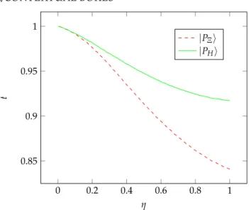
4.4.7 Violation for all non-nullηphotodetection efficiency . . 95

4.4.8 An atom-photon scenario . . . 95

4.4.10 An experimental proposal. . . 98 4.4.11 Possible future directions . . . 100

Conclusions and perspectives 101

Parts of this thesis is based on material published in the following papers:

• [1]Maximal violations and efficiency requirements for Bell tests with photodetection and homodyne measurements

Marco Túlio Quintino, Mateus Araújo, Daniel Cavalcanti, Marcelo França Santos, Marcelo Terra Cunha

Journal of Physics A Mathematical General45,21(2012)215308

Section4.4

• [2] Tests of Bell inequality with arbitrarily low photodetection effi-ciency and homodyne measurements

Mateus Araújo, Marco Túlio Quintino, Daniel Cavalcanti, Marcelo França Santos, Adán Cabello, Marcelo Terra Cunha

Phys. Rev. A86,3(2012)030101

Section4.4

• [3] Realistic loophole-free Bell test with atom-photon entanglement

Colin Teo, Mateus Araújo, Marco Túlio Quintino, Jiˇrí Mináˇr, Daniel Cavalcanti, Valerio Scarani, Marcelo Terra Cunha, Marcelo França Santos submitted –Nature Communications4, (2013)

Section4.4.10

• [4]Complete characterization of the n-cycle noncontextual polytope

Mateus Araújo⋆_{, Marco Túlio Quintino}⋆_{, Costantino Budroni, Marcelo}

Terra Cunha, Adán Cabello

submitted –Phys. Rev. A88,022118(2013)

Section3.5

⋆

These authors contributed equally to this work.

Can we predict the result of a flipped coin?

Our scientific belief suggests that if we know the material of the coin, how it was tossed, and all informations about the wind. . . we could, in principle, predict its result with certainty. But due to our ignorance on these variables, and the complexity of the system, we are forced to describe a flipping coin with probabilities.

As illustrated by one of Einstein’s most famous quotes [5] “Nature doesn’t

know chance, it operates on mathematical principles. As I have said so many times, God doesn’t play dice with the world”, intrinsic probabilistic events causes discomfort in various physicists. Einstein was worried about the probabilities presented on the axioms of quantum mechanics, but at that time, he (and all other physicists) were not aware of one of the most astonishing properties of quantum mechanics, it predictsnonlocalcorrelations. The definition of nonlocal correlations, first published by John Bell in1964, formalises the idea of physical scenarios in which results cannot, even in principle, be predicted with certainty.

Can we decide whether randomness in physical systems is really intrinsic? Are there real life experiments in which probabilities cannot be interpreted as an ignorance of some “hidden variable”? What are the consequences and limitations of this interpretation? The main motivation of this dissertation is to explore the necessary mathematical tools to understand these questions, and also, to answer some of them.

In chapter1we introduce what is known as aBell scenarioby studying col-lections of multivariable probability distributions. We definemultipartite boxes and, using some vocabulary of convex geometry, we discuss the concepts of non-signalisation,quantumness, andnonlocality. Exploring these definitions, we prove the existence of quantum nonlocal boxes and discuss its consequences. We also present some explicit examples in the CHSH scenario, the simplest one that opens room for nonlocality.

In chapter2we present known examples, results, and proof techniques for multipartite boxes. We discuss some concepts of quantum mechanics which allows systems with nonlocal statistics. In order to gain some insights on mul-tipartite boxes, we analyse the CHSH scenario more closely, and present some phenomena that only take place on more complex ones. We end this chapter by discussing one application of nonlocal boxes, cryptographic protocols in which the only assumption necessary for its security is that non-signalling boxes cannot exist. These proposals motivate a class of device independent

protocols, which allows us to infer non-trivial properties of physical systems just by analysing its statistical data.

In chapter3we exploregeneral boxesin what is known as acontextuality scenario, that generalises the idea of a Bell scenario to a wider collection of mul-tivariable distributions. When dealing with general boxes, we overcome the interpretation of different parties pressing buttons, and discuss some simple and natural scenarios that were missed behind the multipartite assumption. We end this chapter by presenting a new result [4]: we analyse then-cycle

scenario and characterise its noncontextual polytope by its tight noncontextu-ality inequalities. This is the first time that a noncontextual polytope is fully described in a scenario with an arbitrary number of settings.

Since we presented and discussed various results on nonlocal/contextual boxes, in chapter4we seek for aBell test, physical realisation of such boxes. We present some previous efforts and itsloopholes, physical assumptions that may not be well justified. After proving some known bounds on efficiency requirements for attaining a loophole free Bell test, we explore them on an ideal physical setup that exhibit nonlocal statistical data. In this setup, we show that maximal quantum (CHSH) violation is attainable [1], and in some

cases we have a CHSH violation even using photodetectors with arbitrarily low efficientcies [2]. We end the chapter by presenting a new proposal of an

Correlations on

N

-partite boxes

Goddoesplay dice.

The main focus of this chapter is to introduce some vocabulary and basic concepts that are explored in the rest of the text. Although all these results and definitions are well known, we hope to clarify and organize then in a consistent notation with the concept ofmultipartite boxes.

1

.

1

Convex geometry

In Euclidean space, a set is convex if given any two points A,B, the line AB joining them lies entirely within that set. Intuitively, this means that the set is connected, in the sense that you connect a segment between any two points without leaving the set, and the set has no dents in its perimeter.

The notion of convex combination is also intimately close to the idea of probabilities: the results of a flipped coin may be understood as a convex combination between head and tails. Since convex geometry definitions are inspired in our everyday geometric experiences in low dimensions1_{, various} theorems sound very natural.

We remark that convex geometry has applications in many branches of science [6,7,8], but here we only provide a brief introduction on the necessary

concepts for studying correlations on boxes. For a more complete starting point, we suggest the classic [9], the first chapter of [10], and the online lecture

notes [11].

Definition1(Convex set). A setC ⊆Rn_{is convex if}

pc1+ (1−p)c2∈ C ∀c1,c2∈ C, and p∈[0, 1].

The dimension of a convex set is the minimal dimension of the Euclidean spaceRd

necessary to describeC.

1_{Usually, inR}2_orR3_.

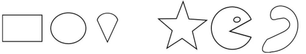
Figure1.1: Three illustrations of convex and three illustrations of non-convex sets.

Definition2(Probability distribution). A distribution associated with K different results is a function p:{i}K

i=1→[0, 1]in which

pi ≥0 and K

∑

i=1 pi =1.

An M-variable distribution is a function p:Ś_m=M ₁{im} →[0, 1]in which pi₁i2...iM ≥0 and

∑

i1i2...iM

pi₁i2...iM =1.

Definition3 (Convex combination). A convex combination of elements ci on a convex setC with distribution p is another element c∈ Cdefined by

c=

∑

i cipi.

In this dissertation we will be interested in what is called aconvex body, bounded closed convex sets with non-empty interior. In other words, convex bodies are the sets that are bounded by (possibly, infinitely) hyperplanes, where a hyperplaneHis a (convex) set of pointsxthat can be represented by a linear equation with real coefficientsai, that is2

H={x∈Rn_|x._{a=b} a∈}Rn, _b∈R. (₁.₁)

Please note that a hyperplane generalizes our notion of plane for any dimension: the equationax+by= 0 inR2represents a line that intercepts

the origin and has an angular coefficient −a/b, the equation z = 0 inR3

represents the standardxyplane.

Convex bodies always contain some special points calledextremal points orpure points, that cannot be written as non-trivial convex combinations of others3_{. Note that pure points always lie in the boundary of the convex set,} but the boundary usually contains non-pure points as well. All non-pure points are calledmixed.

Although we need all extreme points to describe the interior of a convex body as its convex combinations, a single point always can be written as a convex combination ofd+1 extremal points, wheredis the dimension of the convex set. This result is known as Carathéodory theorem and its proof can be found on wikipedia [12] or in any introductory convex geometry book.

2_{Herex.astands for the canonical inner product inR}n_.

3_{A convex combination is trivial if one of the probabilitiesp}

Theorem1(Carathéodory). Any point of a convex bodyC ⊆Rn _{can be written}

as a convex combination of d+1extreme points.

A supporting hyperplane of a convex setC is a hyperplane that intersect C and is such that the all elements ofC lies in one of the closed halfspaces formed by the hyperplane.

Definition4(Supporting hyperplane). LetC ⊆ Rn _{be a convex set, and H}:₌

{x∈Rn_|a._{x=b}be a hyperplane. H is a supporting hyperplane if H andChave}

at least one element in common and the halfspace Hs:={x ∈Rn|a.x≤b}contains C.

The convex hull of a setA ∈Rnis the smallest convex set that contains

A. For example the convex hull of a unit sphereSn−1_:={x∈Rn_{| kxk=1}} is a unit ball Bn _{:={x∈ R}n_{| kxk ≤ 1}, the convex hull of the set of points} V :={(−1,−1),(−1, 1),(1,−1),(1, 1)}is a squareS :={[−1, 1]×[−1, 1]}.

We are now ready for the definition ofconvex polytope.

Definition5(Convex Polytope). A polytope4is a set that can be represented by the convex hull of a finite point subset ofRN_.

Definition6(k-face). LetCbe a convex set andSone of its supporting hyperplanes. The intersectionF := S ∩ C is a face ofC. A face of dimension k is called a k-face and has some special names for some specific values of k: 0-face is a vertex;1-face is an edge; n−1face is a facet.

A set is written inV-representation if its described only by its vertices. By definition, polytopes always admits aV-representation. Our intuition suggests that convex polytopes can be described by its facets as well, that is, its tangent hyperplanes. This intuition is correct, and we call this halfspace description as H-representation. This equivalence between these representations is ensured by the Weyl-Minkowisky theorem, and again, a proof can be found in basic convex geometry books.

Theorem 2(Weyl-Minkowisky). All convex polytopes P ⊆ Rn _{admit a unique}

H-representation with a finite number of linear inequalities.

These two different representations have different applications, and suggest a natural question: how can we obtain theH(V)-representation by knowing the vertex (facet) representation? This problem is known as thevertex (facet) enumeration problem, we’ll see in section1.6that this problem is equivalent5_to a central problem on nonlocality.

1

.

2

Single boxes

We now start our study of correlations, boxes, and probabilities. Before formal definitions, let’s understand some motivation behind it.

4_{Since we are only concerned in convex scenario, we may use the word polytope and convex}

polytope interchangeably.

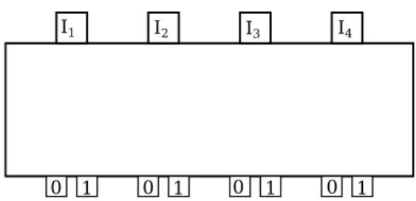
Imagine an experimental setup constructed in a physics lab. Alice, that has no idea on how the experiment was constructed, knows all probabilities to obtain a certain result. To focus on the probabilistic description, we could imagine that the whole experimental setup is inside ablack box6, in which the only thing Alice can do is to press one ofI different buttons, calledinputs, to obtain one ofOdifferentoutputs.

For example, consider a black box with 1 input and 2 outputs conveniently labelled by 0 and 1. This problem is fully described by a random variable that may assume values 0 and 1, and the statistical data of this black box is a probability distribution vector inR2,

p=

p0 p1

.

By trivial generalization we see that anOoutput single button black box can be described by anO-variable distribution vector inRO. Following the

same line, a black box with I different inputs andOdifferent outputs per input7_{is described byIdifferentO-variable distributions, that can be} repre-sented as a vectorRIO. This vector that completely describes the statistical

data of a given experiment will be called asingle box. Adopting the convention8_p

a|Ax for the probability to obtain the outcomea

after choosing the inputAxand labelling the inputs and outputs with natural numbers, a single black box with Iinputs andOoutputs can be described by

p=



    

p_0|A0 . . . p_0|AI−1 p_1|A0 . . . p_1|AI−1

... ... ... pO−1|A0 . . . pO−1|AI−1



    

. (1.2)

Remark1(Representation of distributions). Maybe, the clearest notation for the probability of Alice to obtain the outcome a after choosing the input Ax would be p(Ax= a|Ax), but in more general scenarios this notation easily becomes cumber-some. For the sake of compactness, we will always make the identification

p(Ax=a|Ax)≡ pa|Ax. (1.3)

Remark2(Box representations). Usually, vector space elements are represented by column (or row) matrix, but in this text we will always represent boxes using n×m matrices. For example, in a linear algebra text, the vector p ∈RIO _{represented by}

an I×O matrix in equation(1.2)would probably appear as

p=hp_0|A0 p_1|A0 . . . p_O−1|A0 p_0|A1 . . . p_0|AI−1 . . . p_1|AI−1 p_O−1|AI−1i.

6_{The term black box, borrowed from computer scientists, is used to talk about objects without}

specifying its internal structure.

7_{We could also assume that each input has a different number of outputs, but this}

generaliza-tion has minor interest.

8_{This is an useful compact notation for studying various different distributions. For more}

Please note that our matrix representation is more compact, which is useful for high dimensional vectorial spaces. And in our context, we have the interesting prop-erty that all columns are probability distributions, that is, single boxes are stochastic matrices.

Definition7(Single-box). Let pa|Ax be the probability of Alice to obtain the

out-come a after choosing the input Ax. A single box with I inputs and O outputs is collection of distributions that can be represented by a vector p ∈ RIO _where

elements satisfy

pa|Ax ≥0∀a,Ax,

∑

a

pa|Ax =1 ∀Ax.

The set of all single-boxes that can be constructed with I inputs and O outputs is calledB(I,O).

It is also important to remark that a single box is just a convenient way to express the probabilities of Idifferent random variables that can assumeO different values.

We can easily check that B(I,O) is a convex set: convex combinations of two boxes p andp˜ always satisfies the positivity and the normalisation

condition:

∑

a

tpa|Ax + (1−t)p˜a|Ax

=t

∑

a

pa|Ax

+ (1−t)

∑

a

˜ pa|Ax

=

=t+1−t =1.

And by noting that a point of this convex set is pureiff it represents a box with a deterministic probability distribution9_{, we see thatB(I,O)is a convex} polytope.

1

.

3

Bipartite boxes

Imagine now Alice shares one black box experiment with Bob. That is, in a different laboratory, Bob has access toIBdifferent input buttons and may haveOB different output results. Now, we also assume that Alice and Bob only obtain their outputs after both press their input buttons10

A complete description of this bipartite scenario must specify all probabili-ties pab_|AxBy of Alice and Bob obtaining the resultsaandbwhen they press

AxandBy. This can be made by specifying the probabilities ofIAandIB, two variable distributions that can assumeOA, andOBdifferent values. As in a

9_{A probability distribution is deterministic if contains only zeros and ones.}

10_{We also implicitly assume that the time order of pressing buttons does not affect the outputs,}

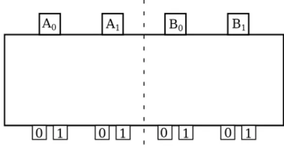
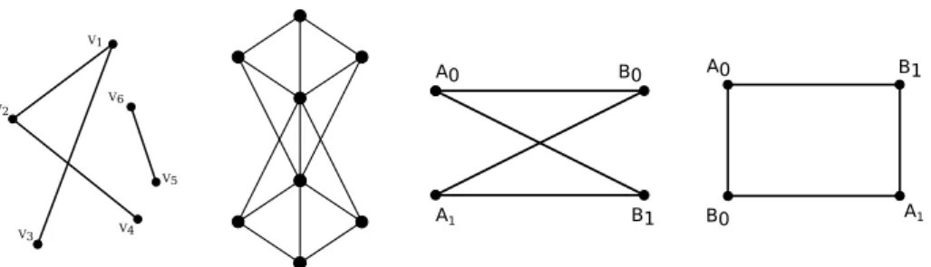
A0 A1 B0 B1

0 1 0 1 0 1 0 1

Figure1.2: A box illustrating the scenario(2, 2, 2), more discussed on section 1.8.

single box scenario, we represent this probabilities in a vector inRIAIBOAOB,

p=



    

p_00|A0B0 . . . p_00|A

IA−1B_IB−1 p_01|A0B0 . . . p01|A_IA−1B_IB−1

... ... ...

pOA−1,OB−1|A0B0 . . . pOA−1,OB−1|A_IA−1B_IB−1



    

. (1.4)

Definition8 (Bipartite scenario). LetIA ={Ax}IA

1 ,OA ={a}O1A be the set of inputs/outputs of Alice andIB={By}IB

1,OB={b}O1B be the set of inputs/outputs of Bob. The4-tupleS = (IA,OA;IB,OB)is a bipartite box scenario.

Since the label of inputs and outputs has no deep meaning, we also use the short-hand notationS = (IA,OA;IB,OB), and for the case where IA= IBand OA =OB we just writeS = (2,I,O).

Definition 9 (Bipartite box). Let p_ab|xy be the probability of Alice and Bob ob-taining the outcomes a and b when they press Ax and By, respectively. A bipartite box in the scenarioS = (IA,OA;IB,OB)is a collection of distributions that can be described by a vectorp∈Rd_{(d=IAIBOAOB)in which elements satisfies}

pab|AxBy ≥0∀a,b,Ax,By,

∑

a,b

pab|AxBy =1 ∀ Ax,By. (1.5)

The set of all bipartite boxes that can be constructed in a specific scenario isB(S). For the case where IA= IBand OA=OBwe just writeB(2,I,O).

As in the single box scenario, bipartite boxes are just one convenient way to write a set of two variable probability distributions. And the set B(IA,OA;IB,OB)is the convex hull of all bipartite deterministic boxes.

Definition10(Marginal probability). The marginal probabilities p_a|Ax;By of a two variable distribution with coefficients pab_|AxBy is

pa|Ax;By :=

∑

b

pab|AxBy.

We also define the marginal probabilities pb|By;Ax as

p_b|By;Ax :=

∑

a

p_ab|AxBy.

Remark 3. Maybe, the clearest notation for the probability of Alice and Bob to obtain the outcomes a and b when they press Axand Bywould be p(Ax=a,By= b|Ax,By). So the marginals would be defined as

p(Ax=a|Ax,By):=

∑

p(Ax=a,By=b|Ax,By);

p(By=b|Ax,By):=

∑

p(Ax=a,By=b|Ax,By).

But for the sake of compactness we will always make the identifications p(Ax=a,By=b|Ax,By)≡pab|AxBy;

p(Ax=a|Ax;By)≡pa_|Ax;By;

p(By=b|Ax;By)≡pa_|By;Ax.

Intuitively, a two variable distribution is uncorrelated if we can describe it only by its marginals. More formally, a two variable distribution p_{. .|}AxBy is

completely uncorrelated if, for each fixedx,y,

p_ab|AxBy = p_a|Ax;Byp_b|By;Ax ∀a,b. (1.6) It is interesting to note that deterministic two variable distributions are al-ways uncorrelated, to prove this we just need to use the fact that deterministic distributions only have events of probability zero or one. So randomness is a necessary condition for correlations between two variable distributions.

In order to gain some interpretation on correlations it is interesting to invoke a simple result from probability theory.

Theorem 3. For any fixed x,y, a two variable distribution p_{. .|}AxBy that can

as-sume OAdifferent values on the first variable and OBdifferent values on the second variable can be written as

p_ab|AxBy =

∑

λ

πxy(λ)p_a|Ax;λp_b|By;λ (1.7)

Proof. The set of all two variable distributions that can assumeOA different values on the first variable andOBdifferent values on the second variable is a convex polytope withOAOBdeterministic distributions as vertices. Now we use deterministicp_.|A;λand p.|B;λto construct the vertices of the two variables

distribution polytope via the product of marginals pab|AxBy;λ:= pa|A;λpb|B;λ.

Since all points inside a polytope can be written as convex combinations of its vertices, all two variable distributions can be written in the form of pab_|AxBy = ∑λπxy(λ)pab|AxBy;λ. We we guarantee the existence of a setΛxy

with cardinalityOAOB+1 by invoking Carathéodory theorem. The equation (1.7) allows the interpretation:

In principle, all two-variable distributions are uncorrelated and deterministic, probabilities arise as an ignorance onλ.

Due to this interpretation,λis usually referred as ahidden variable, since we are forced to work with probabilities because we cannot have access to its value.

Since bipartite boxes are just a collection of two variable distributions, theorem3has two natural extensions for bipartite boxes.

Corollary1. All probabilities of bipartite boxes admit the representation pab|AxBy =

∑

λ

πxy(λ)pa|Ax;λpb|By;λ (1.8)

for some distributionsπxy:Λxy→[0, 1], and one variable distributions p_.|Ax;λand

p_.|By;λ.

Corollary2. All probabilities of bipartite boxes admit the representation pab|AxBy =

∑

λ

π(λ)pa|Ax;Byλpb|By;Axλ (1.9)

for some distributionπ : Λ _{→[0, 1], and one variable distributions p.|A}

x;Byλ and

p_.|By;Axλ.

Proof. To prove this corollary we just need that, since the distributions of the vertices of the bipartite box polytopeB(2,I,O)are deterministic, they can always be written as

pab|AxBy =pa|Ax;Byλpb|By;Axλ,

by settingp_a|Ax;Byλandp_b|By;Axλas deterministic. Now, it follows by convexity that all probabilities of bipartite boxes can be written in the form of1.9.

1

.

3

.

1

Non-signalling

Consider a two output, two input, deterministic bipartite box defined by

p_00|A₀B₀ =1, p10|A₀B₁ =1, p01|A₁B₀ =1, p11|A₁B₁ =1. (1.10) Other equivalent (and possibly, more enlightening) way to define this box is writing11

a=y,b=x,

that is, Alice’s output is Bob’s input, andvice versa. Can we ask questions like “What is the probability of Alice to obtain 0 while she pressesA0?”?

From marginal probabilities, we know that the probability of Alice obtain-ing 0 while she presses A0depends on Bob’s choiceBy. Ify=0, Alice obtains 0, ify=1, she obtains 1. So, ifp_0|A0;B0 6=p0|A0;B₁, Alice’s probability to obtain 0 as pressingA0,p0|A0, may not have a precise meaning.

A natural question is, when can we talk about p_0|A0? Well, if Alice’s marginal probabilities satisfy p_0|A0;B0 = p0|A0;B1, it is fair to define p0|A0 := p_0|A0;B0 =p_0|A;0B1. This condition is callednon-signalling.

Definition11(Non-Signalling). A bipartite box is non-signalling if its probabili-ties satisfy12

∑

b

pab|AxBy =

∑

b

pab|AxBy′ := pa|Ax ∀a,Ax,By,By′

∑

a

pab_|AxBy =

∑

a

pab_|A_x′By :=pb|By ∀b,Ax,Ax′,By (1.11)

The set of all non-signalling bipartite boxes is denoted byN S(IA,OA;IB,OB), or justN S(2,I,O)in case IA =IBand OA=OB.

Remark 4. Using the clear notation p(Ax=a,By=b|Ax,By) suggested in re-mark3we see that the non-signalling condition allows us suppress the indexes|Ax, |Byin our notation. That is, without ambiguity, we can write

p(Ax=a):=p(Ax=a|Ax) =:p(Ax=a|Ax,By); p(By=b):=p(By=c|By) =:p(By=b|Ax,By); p(Ax=a,By=b) =:p(Ax=a,By=b|Ax,By).

In the non-signalling scenario, we can understand Ax and Byas usual random variables. We will see in chapter3that the existence of the probabilities p(Ax=a) and p(By=b)are the conditions imposed in a what we call a marginal scenario.

Informally, non-signalling is a necessary and sufficient condition for talking about two “individual” parts13_{, if Alice presses the input buttonA}

x, she can obtain an outputaxindependently of weather Bob pressed a button or not14.

11_{In fact, all deterministic boxes admit this input/output representation.}

12_{We remark that some authors refer tor non-signalling bipartite boxes asbehaviours. This}

term was coined in one of Tsirelson’s seminal papers [13].

13_{In signalling boxes, we have no rights to talk about individual parts, because one side can}

“manipulate” the other probabilities by exploringp_a|Ax;By6=pa|Ax;By′.

14_{In information theory [14] this means that this box cannot be used for communication. That}

It is very important to remark that the non-signalling condition does not forbid correlations, we can still havepab_|AxBy 6= pa|Axpb|By. One good example

is theperfect correlated, that in the box in the scenario where Alice and Bob have two outputs, can be defined as15

p00|AxBy = p11|AxBy =1/2.

We can check that all distributions of this boxes are correlated, p_ab|AxBy 6= pa_|Axpb|By , and also the non-signalling condition holds true:

p_00|AxBy +p01|AxBy =p00|AxB′y+p01|AxB′y =1/2 ∀x,y,y

′_;

p_00|AxBy +p_10|AxBy =p_00|A′_xB′_y+p_10|A′_xB′_y =1/2 ∀x,x′,y.

Another important remark is that the linearity of equations16_{(1.11) ensures} thatN S(IA,OA;IB,OB)is a polytope17.

1

.

3

.

2

Local

For those who knowλ, there are no

correlations.

Theorem3 ensures the classical intuition that all correlations between probabilities arise as a possible ignorance from an inaccessible information. What can we say about box correlations?

Before exploring box correlations, it is important to have a good compre-hension of distribution correlations. Suppose Eve prepares a bipartite single input box18_{,p∈ B(2, 1, 2)using the following rule: she flips a coin; if heads,} she outputs 0 for Alice and 1 for Bob; if tails she does the opposite. Assuming that the only source of uncertainty in this experiment is Eve’s coin’s result, and that the coin returns heads with probability19 _{p(h), without knowing the} result of Eve’s coin, Alice and Bob’s best description of this box is

pab=p(h)pa|A;hpb|B;h+p(t)pa|A;tpb|B;t, (1.12) or more explicitly

p00 =p(h)p0|A;hp0|B;h+p(t)p0|A;tp0|B;t=0; p01 =p(h)p0|A;hp1|B;h+p(t)p0|A;tp1|B;t=p(h); p10 =p(h)p1|A;hp0|B;h+p(t)p1|A;tp0|B;t=p(t);

p11 =p(h)p1|A;hp1|B;h+p(t)p1|A;tp1|B;t=0. (1.13)

15_{Also note that the normalisation condition that implies thatp}

01|AxBy=p10|AxBy=0

16_{For real numbers,a=b ⇐⇒ a≥b, anda≤b.}

17_{Intersections of a polytope with a finite number of hyperplanes is also a polytope.} 18_{Although single input bipartite boxes are just two-variable probability distribution, we chose}

this notation for further generalization.

These equations say that Alice and Bob cannot predict their outcome with certainty only because they do not have access to the coin’s result. In principle, Eve (and/or others) can describe the whole experience by p_01|h = 1 and p_10|t=1. In fact, we will later prove that Eve can construct (and then foresee the results with certainty) all single input bipartite boxes just by flipping coins.

What can we say about general bipartite boxes? From corollary2we can writep_ab|AxBy =∑_λπxy(λ)p_a|Ax;λp_b|By;λ, but we need various differentπ..|xy distributions that depend on Alice and Bob’s input choice. This means that in the general case, Eve must know their inputs to construct a bipartite box. One could ask: what class of boxes can Eve construct if she cannot have access to Alice and Bob’s inputsAxandBy?

Definition12(Locality). A bipartite box is local if all probabilities can be written as

pab_|AxBy =

∑

π(λ)pa_|Ax;λpb|By;λ ∀a,x,y,y′, (1.14)

for some distribution π : Λ _{→ [0, 1] and single variable distributions pA}

x;λ and

pBy;λ.

The set of all local bipartite boxes isL(IA,OA;IB,OB), or justL(2,I,O)in case IA=IBand OA =OB.

This definition was first presented in John Bell’s1964seminal paper [15].

Bell was motivated by studying correlations that have a same common cause: the distributionπoverλ.

It must be clear that, for local boxes, we can always define Alice’s marginal probabilities regardless of Bob’s choice. That is, all local boxes are non-signalling.

Theorem4. L(IA,OA;IB,OB)⊆ N S(IA,OA;IB,OB).

Proof. Since the role of Ax andBy is symmetric in both definitions, we just need to prove that if we assume equation (1.14), the marginal p_a|Ax;By does not depend onBy. Explicitly:

pa_|Ax;By :=

∑

b

pab_|AxBy

=

∑

bλ

π(λ)p_a|Ax;λp_b|By;λ; =

∑

λ

π(λ)p_a|Ax;λ(

∑

b

p_b|By;λ);

=

∑

λ

π(λ)pa|Ax;λ.

Theorem5(20).

B(2, 1,O) =L(2, 1,O);

L(IA,OA;IB, 1) =N S(IA,OA;IB, 1); L(1,OA;IB,OB) =N S(1,OA;IB,OB).

This theorem follows as a corollary of theorem22, to be proved on chapter 3. In fact, this theorem is even stronger. These particular scenarios are the only ones in which non-signalling implies locality. It may be surprising to know that there are nonlocal boxes that respect the non-signalling condition, in section1.8we will illustrate this fact in the(2, 2, 2)scenario.

We now exhibit an equivalent definition for local boxes that explore the vectorial character of box spaces.

Theorem6. A bipartite boxp∈ B(IA,OA;IB,OB)is localiffit can be written as

p=

∑

λ

π(λ)pλ_A⊗pλB, (1.15)

whereπ:Λ_{→[0, 1]is a distribution, p}λ

A∈ B(IA,OA), andpλB∈ B(IB,OB). Proof. To prove this theorem we just need to recognize that the components of pare exactly

pab|AxBy =

∑

π(λ)pa|Ax;λpb|By;λ.

This simple theorem provides an interesting parallel between nonlocality andquantum entanglement. In section2.1we define quantum entanglement and present a brief discussion on this analogy.

Before ending this section, we make an important connection between deterministic non-signalling boxes and local boxes.

Theorem 7. A bipartite box is local iff is a convex combination of bipartite non-signalling deterministic boxes.

Proof. As proved before, all local boxes are non-signalling, so we only need to prove that convex combinations of non-signalling deterministic boxes are local.

Since any deterministic two variable distribution is completely uncorre-lated, any deterministic non-signalling box has the probabilities in the form

pab|AxBy;λ =pa|Ax;λpb|By;λ.

Now, we just check that convex combinations of these probabilities is exactly the definition of locality,

∑

λ

π(λ)pab|AxBy;λ =

∑

π(λ)pa|Ax;λpb|By;λ.

20_{It may be useful to recall thatS= (N,I,O)represents a scenario withNparties,Iinputs}

per party, andOoutputs per input, andS′ _{= (IA,OA;IB,OB)represents a bipartite scenario}

Corollary3. The set of local boxes is a convex polytope in which vertices are deter-ministic non-signalling boxes.

Due to this fact, the set of all bipartite local boxes is also known as the local polytope.

1

.

3

.

3

Quantum

How can we describe boxes that represent quantum experiments? In other perspective, what class of boxes can Eve prepare with quantum systems? The ones who are familiarised with quantum mechanics may say: “we just need to prepare a certain quantum state and choose some measurement operators, then the probabilities to obtain a certain output will be given by the quantum measurement postulate”. And that is exactly the definition of quantum boxes, the ones that can be constructed by measurements on quantum systems.

We will now define all quantum objects that are necessary for under-standing quantum boxes, but nothing more than that. Readers that do not feel comfortable with quantum mechanics are invited to read Nielsen and Chuang’s book [16], or for introductions to quantum mechanics more focused

on nonlocality we suggest [17,18,19,20].

Definition13(Quantum Theory). LetHnbe an n-dimensional Hilbert space over

C_{. A quantum state is a trace}1_{positive semidefinite}21_{linear operatorρ}:_{Hn→ Hn.}

A set of operatorsM={Mi}is a quantum measurement set if all Mi :Hn → Hnare positive semidefinite operators that sumf to identity,∑_iMi =I.

The probability to obtain the result i after subjecting the stateρ to the quantum measurementMis p_i|ρM=trρMi_.

We are now able to define bipartite quantum boxes.

Definition14(Quantum Boxes). A bipartite box is quantum if each probability can be written as

p_ab|AxBy =tr(ρABAax⊗Byb) ∀a,b,x,y,

for a certain quantum stateρAB :Hn⊗ Hm → Hn⊗ Hmand quantum measure-ment setsAx={Aix}, Aix:Hn → Hn andBy={B

j

y},Byj :Hm→ Hm.

The set of all quantum bipartite boxes is calledQ(IA,OA;IB,OB), or justQ(2,I,O) in case IA= IBand OA =OB.

Please note that this definition does not specify the dimension of the Hilbert space associated to the quantum system, that is, to understand Q(IA,OA;IB,OB) we may need to deal with infinite dimensional vector spaces22_.

Quantum measurements on one single part23 _{cannot alter the results on} the other one. In our text, this means that bipartite quantum boxes are non-signalling.

21_{An operatorρ:H}

n→ Hnis positive semidefinite if satisfieshv,ρvi ≥0,∀v∈ Hn.

22_{In fact, in [21] the authors suggest that some quantum boxes need measurements on infinite}

dimensions to be constructed.

23_{They are also calledlocal measurements, and are represented by measurement operators that}

Theorem8. Q(IA,OA;IB,OB)⊆ N S(IA,OA;IB,OB).

Proof. The proof follows from a straightforward calculation that checks that all boxes p ∈ Q(IA,OA;IB,OB)satisfy the conditionspa|AxBy = pa|AxBy′, and

p_b|AxBy = p_b|A′_xBy:

pa_|AxBy =

∑

b

pab_|AxBy;

=

∑

b

tr(ρABAax⊗Bby);

=tr(ρABAax⊗(

∑

Byb)); =tr(ρABAax⊗(I)).

Also, all local boxes can be simulated by quantum systems. Before proving that fact, we would like to explicitly show that all probability distributions can be simulated by measurements on quantum systems.

Theorem9. All multivariable probability distributions p can be simulated by per-forming measurements on quantum systems.

Proof. For simplicity, we will first assume thatpis a single variable distribution represented by probabilities{pi}K_i=1.

Define quantum a stateρ:HK→ HKand quantum measurement opera-tors Mj_{:HK→ HK}

ρ= K

∑

i

piΠi, Mj =Πj,

where {Π_i}K

1 is a set of unidimensional orthogonal projectors. Now, by straightforward calculation we can check that these operators define a valid quantum system24_{and trρM}i _=p

i.

For multivariable distributions, we can use exactly the same technique, we just need to enlarge our Hilbert space.

Theorem10. L(IA,OA;IB,OB)⊆ Q(IA,OA;IB,OB).

Proof. Just note that it is possible to construct a quantum state and some measurement operators to obtain any local box probabilities. For example, we can always use the state

ρAB=

∑

λ

π(λ)ρλA⊗ρλB

and measurement operators that satisfy (see theorem9)

tr(ρλAAxa) =pa|Ax;λ, and tr(ρ λ

BB y

b) =pb|By;λ,

to obtain

tr(ρABAxa⊗B y b) =

∑

λ

π(λ)pa_|Ax;λpb|By;λ.

Although all local boxes are quantum, there are nonlocal quantum boxes. This result is known as Bell’s theorem25_{[15], and has some deep consequences} on foundations of quantum mechanics. The first immediately consequence is the absence of generalization of theorem7: some quantum systems cannot be described by convex combinations of deterministic boxes.

The setQ(IA,OA;IB,OB)is convex [22,23], but differently from previously discussed box sets, it is not a polytope26_{. This fact makes the structure of} quantum box sets much more complex.

Theorem11. The setQ(IA,OA;IB,OB)is convex.

Proof. We need to show that if p1,p2 ∈ Q(IA,OA;IB,OB), thenλp1+ (1− λ)p2∈ Q(IA,OA;IB,OB).

Ifp1,p2∈ Q(IA,OA;IB,OB), there are quantum statesρ1,ρ2:Hn⊗ Hn → Hn⊗ Hn and quantum measurements operatorsAix,a,Byj,b :Hn → Hn such that

p1_ab|AxBy =tr(ρ1A1,xa⊗B1,yb); p2_ab|A

xBy =tr(ρ

2_A2,a

x ⊗B2,yb).

Now, we define a state ˜ρ : H2n⊗ H2n → H2n⊗ H2n and measurement operators ˜Aa_x, ˜B_yb:H2n→ H2n as

˜

ρ:=λρ1⊗Π1_⊗Π1_{+ (1−λ)ρ}2_⊗Π2_⊗Π2_;

˜

Aax:= A1,xa⊗Π1+A2,xa⊗Π2; ˜

Bxa:=By1,b⊗Π1+B2,yb⊗Π2,

whereΠ1_,Π2 : _{H2 → H2 are orthogonal unidimensional projectors. Now}

we check that the probabilities of this new quantum system are exactly the convex combination of the older ones,

˜

p_ab|A˜xB˜y =tr(ρ˜A˜

a

x⊗B˜yb) =

=λtr((ρ1⊗Π1_⊗Π1_)[(A1,_xa_⊗Π1_+A2,_xa_⊗Π2_)⊗(B1,_yb_⊗Π1_+B2,_yb_⊗Π2_)])

+ (1−λ)tr((ρ2⊗Π2_⊗Π2)[(B1,_xa⊗Π1+B_x2,a⊗Π2)⊗(B1,_yb⊗Π1+B_y2,b⊗Π2)]) =λtr(ρ1A_x1,a⊗B_y1,b) + (1−λ)tr(ρ2A2,_xa⊗B2,_yb)

=λp1_ab|A

xBy+ (1−λ)p

2 ab|AxBy.

So we can always construct a quantum box that provides us the probabilities of the convex combinationλp1+ (1−λ)p2.

25_{Some times also stated in phrases like “Quantum mechanics is a nonlocal theory”, or}

“Quantum mechanics cannot be described by local hidden variables”.

26_{In section1.8we will see thatQ(I}

Please note that we explored the freedom on the vector space dimension to prove the convexity ofQ(IA,OA;IB,OB). In fact, if we require quantum states to lie in a Hilbert space with a fixed dimension, the set of quantum boxes may not be convex [24].

1

.

4

General properties on bipartite box sets

Before starting with multipartite boxes, we summarize some important prop-erties of bipartite box sets. We also anticipate that these propprop-erties still hold for the multipartite scenario.

• They respect the hierarchical relation

L(S)⊂ Q(S)⊂ N S(S)⊂ B(S),

where,_S = (IA,OA;IB,OB)is a bipartite scenario with more than one output and input per part27_.

• All previous bipartite box sets are convex.

• Except from the quantum, all sets are polytopes.

1

.

5

Multipartite scenario

All previous concepts developed for bipartite boxes will be now generalized for anN-partite scenario. AsNgrows, the number of possibilities on signalization and nonlocality became larger. And although most generalizations are quite natural, some difficulties may appear due to a necessarily heavy notation. In order to help the readers to visualise multipartite boxes, we will provide illuminating examples.

1

.

5

.

1

Multipartite boxes

In the bipartite scenario, we allowed each part to have different number of outputs and inputs. This freedom has minor interest and may lead us into very cumbersome notation. So, for practical reasons, we will now assume that each part has access toIdifferent inputs andOdifferent outcomes per input.

Definition15(Multipartite scenario). LetIn = {in}I

i=1,On ={on}O_o=1be the set of inputs/outputs of the party n. The 3-tuple S = (N,{In}N_,{On}N_{) is a} multipartite box scenario.

Since the label of inputs and outputs has no deep meaning, we also use the short-hand notationS = (N,I,O).

Definition16(Multipartite box). Let

po|i:= po₁o2...oN|1i₁2i₂...N_iN

be the probability of the parties1,2, . . . , N to obtain the outcomes o1, o2, . . . , oN, after they chose (respectively) the inputs i1, i2, . . . , iN. An N-partite box in the scenario (N,I,O) is a collection of distributions that can be described as a vector p∈Rd_{(d= (IO)}N_{)in which elements satisfy}

po|i≥0 ∀o,i,

∑

po|i=1 ∀i. (1.16)

The set of all N-partite boxes that can be described with I inputs and O outputs isB(N,I,O).

As in the bipartite scenario, the setB(N,I,O) is the convex hull of de-terministic multipartite boxes, and its elements are just a convenient way of representing IN _{differentN-variable distributions.}

The definition of marginal probabilities for N-variable distributions is completely analogous to the two variable ones, except by the difference that more variables allow to talk about more marginal possibilities. Let us take a closer look at the tripartite case.

The number po1o2o3|1i₁2i₂3i₃ represents the probability of parts 1, 2, 3 to

obtain the outputso1,o2,o3, after pressingi1,i2,i3. The distributionp1i₁2i₂3i₃

can provide us6different marginal probabilities:

p_o1|1i

1;2i₂3i₃ :=

∑

o2o3

p_o1o2o3|1i 12i₂3i₃;

po2|2i₂;1i₁3i₃ :=

∑

o1o3

po1o2o3|1i₁2i₂3i₃;

p_o3|3i

3;1i₁2i₂ :=

∑

o1o2

p_o1o2o3|1i 12i₂3i₃;

p_o1o2|1i

12i₂;3i₃ :=

∑

o₃

p_o1o2o3|1i 12i₂3i₃;

po2o3|2i₂3i₃;1i₁ :=

∑

o1

po1o2o3|1i₁2i₂3i₃;

po1o3|1i₁3i₃;2i₂ :=

∑

o2

po1o2o3|1i₁2i₂3i₃.

Before moving to the general definition, we remark some possible notation issues.

Remark 5. As in po|i = po1o2...oN|1i₁2i₂...N_iN, we are going to use bold letters for

representing a list of variables.

• lwill represent parties involved, for examplel =2, 3, 5represents the parties 2,3, and5.

• l¯is the complement ofl, for example ifl=2, 3, 5, then_l¯_{=1, 4, 6, . . . ,N.}

• The setOlis the set of all possible outcomes related to the listl.

Definition 17 (Marginal probability). Given an N variable distribution with coefficients po|iand a listlwe define the marginals as

p_ol|il;i¯

l :=

∑

1

.

5

.

2

Non-signalling boxes

Definition18(Non-Signalling). An N-partite boxp∈ B(N,I,O)is non-signalling if the marginal probabilities for all list of partiesldo not depend on the other parties

¯

linput choices. That is, all marginals can be written as p_ol|il;i¯

l = pol|il.

The set of all non-signalling boxes with N parties, I inputs per party, and O outputs per input is denoted byN S(N,I,O).

One interesting theorem proved in [19] states that if all marginals with

N−1 variables are non-signalling, the whole box is NS. For example, in a tripartite scenario, if 1 cannot signal to 2 and 3 and that 2 cannot signal to 1 and 3, we deduce

∑

o₁,o2

po₁o₂o_3|i₁i₂i₃ =

∑

p_o1o2o3|i′

1i2i3 ∀o3,i′1i1i2i3 =

∑

o1,o2

po₁o2o3|i′₁i′₂i3 ∀o3,i′1i1i′2i2i3,

(1.18)

which is the condition that 1 and 2 cannot signal to 3.

Another important remark is that, like in bipartite scenarios,N S(N,I,O) is a convex polytope and a multipartite box can be used for communicationiff is signalling.

1

.

5

.

3

Local boxes

Definition19(Locality). An N-partite box is local if all probabilities can be written as

p_o|i =

∑

λ

π(λ)p_o1|1i

1;λpo2|2i₂;λ. . .poN|N_iN;λ ∀o,i, (1.19)

for some distributionπ:Λ_→[0, 1]and single variable distributions px_ix;λ.

The set of all local multipartite boxes with N parties, I inputs per party, and O outputs per input is denoted byL(N,I,O).

We also remark that _L(N,I,O) is the convex hull of all non-signalling deterministic boxes, and it is also called aslocal polytope. Also, the parallel with quantum entangled states still remains: a multipartite box is nonlocaliff it cannot be written as convex combination of tensor product of single boxes, p = ∑_λπ(λ)p₁λ⊗pλ₂⊗. . .pλ_N. The proof of these theorems are completely analogous to the ones proved for bipartite boxes.

1

.

5

.

4

Quantum boxes

The boxes that we can construct with quantum systems follow from simple generalization. Also all other properties presented for the bipartite scenario still remain: quantum multipartite boxes form a convex set with infinitely many extremal points and respectL(N,I,O)⊆ Q(N,I,O)⊆ N S(N,I,O).

Definition20(Quantum boxes). An N-partite box is quantum if each probability can be written as

po|i=tr(ρ1o11i ⊗2

o2

2i ⊗. . .⊗N

oN

N_i) ∀o,i,

for a certain quantum state ρ : H⊗N

n → H⊗nN and quantum measurement sets 1x = {1o₁1_i},1₁o1_i : Hn → Hn,2x = {2₂o2_i},2o₂2_i : Hn → Hn, . . . , Nx = {No_NN_i},

NoN

Ni :Hn→ Hn.

The set of all quantum N-partite boxes with I inputs per party and O outputs per input isQ(N,I,O).

1

.

5

.

5

General properties of multipartite box sets

As stated in section1.4, multipartite boxes also obey some general properties.

• They respect the hierarchical relation

L(S)⊂ Q(S)⊂ N S(S)⊂ B(S),

where,S = (N,I,O)is a multipartite scenario with28 _I,O≥2. • All previous multipartite box sets are convex.

• Except from the quantum, all sets are polytopes.

1

.

6

Bell inequalities and the facet enumeration problem

When satisfied they indicate that the data may have, when not satisfied they indicate that the data cannot have, resulted from actual observation [29].

George Boole

Given all probabilities of a certain box, how can we decide if this box is local, in the sense of definition (19). Geometrically, given p∈ B(N,I,O), how to decide whenever p∈ L(N,I,O)?

The problem of deciding if a certain p lies inside a polytope is famous in computational geometry. One way to solve it is to check ifp satisfies all halfspace inequalities. Theorem7guarantees that the vertices of the local polytope are the non-signalling deterministic boxes. So, we can reduce our

question to the facet enumeration problem, that is, to find theH-representation of a convex polytope.

There is an algorithm based on the Fourier-Motzkin elimination29 _that transforms the V-representation into the H-representation [32]. Moreover,

there is a algorithm implemented in C that performs this transformation [33],

so the problem of finding all facet inequalities is, in some sense, solved. We said in some sense because the time computational complexity of the best known algorithm for solving this problem is30 _O(d!Vd_{)[35], whereVstands} for the vertex number anddis the dimension of the polytope31_.

In complexity theory, algorithms that have exponential complexity are non-efficient32_{. Readers that are not familiar with computation may take the} following rule of thumb: “Non-efficient algorithms takes a very long time to be solved even with very good computers”. If the best known algorithm to solve a certain problem is non-efficient, this problem is said to be computationally hard [36].

1

.

6

.

1

The facets of the local polytope

The first ideas on exploring correlation sets as convex polytopes were proposed by Froissart in 1981[37]. It took 12 years until someone (Boris Tsirelson) explored these geometric aspects on nonlocality [13]. But now, almost all

papers on nonlocality use this geometric vocabulary.

Due to John Bell’s seminal paper on non-locality [15], the hyperplanes that

describe the local polytope are calledBell inequalities.

Definition21(Bell inequalities). The linear inequalities that are respected by all local boxes are called Bell inequalities.

Inequalities that are equivalent to the positivity, normalisation, or non-signalling condition (equations(1.5)and(1.11)), are said to be trivial.

Bell inequalities defining facets are called tight.

We could not end this section without commenting the very curious fact that pioneer papers on nonlocality were published without mentioning that Bell inequalities actually date back to 1862, due to George Boole’s works [29,38]. Most famous for his contributions to mathematical logic, Boole also

has some papers on probability in which he considered the question: How can we decide if a certain set of probabilities came from a valid statistical data. Immersed in a classical scenario, Boole could not think that a nonlocal set of probabilities might be physically possible, and after finding his inequalities he wrote:

29_{The first register to this algorithm dates back to1826, in a work by Fourier [30]. Without}

knowing Fourier results, Motzkin rediscovered it1936in his thesis [31].

30_{We also remark the existence of a discussion on how should we measure the complexity of}

this problem [23,34].

31_{In section1.10we will see that the dimension of the polytope grows exponentially in the}

number of parts. So the complexity of our main problem is even larger.

32_{An algorithm is efficient if, in the worse case, its time-complexity has a polynomial}