xx/xx
J. Aerosp. Technol. Manag., São José dos Campos, v10, e3618, 2018
doi: 10.5028/jatm.v10.934 ORIGINAL PAPER
1.Malek-Ashtar University of Technology – Department of Mechanical and Aerospace Engineering – Shahinshahr/Isfahan – Iran
Correspondence author: Ali Babaei | Malek-Ashtar University of Technology – Department of Mechanical and Aerospace engineering | Ferdowsi Street – Malek-Ashtar University of Technology | CEP: 83.145-115 – Shahinshahr/Isfahan – Iran | E-mail: [email protected]
Received: Jun. 4, 2017 | Accepted: Sept. 19, 2017 Section Editor: Paulo Greco
ABSTRACT: In this study, an efficient methodology is proposed for robust design optimization by using preference function and fuzzy logic concepts. In this method, the experience of experts is used as an important source of information during the design optimization process. The case study in this research is wing design optimization of Boeing 747. Optimization problem has two objective functions (wing weight and wing drag) so that they are transformed into new forms of objective functions based on fuzzy preference functions. Design constraints include transformation of fuel tank volume and lift coefficient into new constraints based on fuzzy preference function. The considered uncertainties are cruise velocity and altitude, which Monte Carlo simulation method is used for modeling them. The non-dominated sorting genetic algorithm is used as the optimization algorithm that can generate set of solutions as Pareto frontier. Ultimate distance concept is used for selecting the best solution among Pareto frontier. The results of the probabilistic analysis show that the obtained configuration is less sensitive to uncertainties.
KEYWORDS:Robust design, Optimization, Fuzzy logic, Preference functions.
INTRODUCTION
Engineering design cycle is a process of the subsystems formulation to meet human needs. To increase design performance, it is necessary to use the design optimization methodologies in the systems design (Hao et al. 2015). Complex systems usually have multiple conflicting disciplines, which difficult its compromise. Moreover, sequential or single objective optimization will result in low-efficiency solutions or even non-optimal solutions (Huang et al. 2008). Multi-objective optimization is a method that optimizes a group of objective functions simultaneously (Huang et al. 2006).
In today’s world, systems should also be robust in the face of uncertainties. In other words, the performance of the optimal solutions must have fewer changes because of the variations of design variables and operational conditions. So a measure of robustness should be introduced during optimization and design (Gaspar-Cunha and Covas 2008). Taguchi introduces robust design at first to enhance product quality so that the quality is not sensitive to variations (Wan et al. 2011). The purpose of this method is to minimize the deviation of system response due to uncertainties. In classical design methods for considering uncertainty in a system design, the designers apply drastic tolerances and large safety factors (Jun et al. 2011). Assigning the values of these parameters is based on past experience of designer and has these drawbacks: a) specifying the values of safety factor for new systems and materials without any experience is difficult; b) in the design process, it is not easy to measure robustness and
A New Approach for Robust Design
Optimization Based on the Concepts of
Fuzzy Logic and Preference Function
Ali Reza Babaei1, Mohammad Reza Setayandeh1
Babaei AR; Setayandeh MR (2018) A New Approach for Robust Design Optimization Based on the Concepts of Fuzzy Logic and Preference Function. J Aerosp Technol Manag, 10: e3618. doi: 10.5028/jatm.v10.934.
How to cite
Babaei AR http://orcid.org/0000-0002-8092-2931
J. Aerosp. Technol. Manag., São José dos Campos, v10, e3618, 2018 Babaei AR; Setayandeh MR
xx/xx 02/22
reliability, so the designer cannot compare the system from standpoint of resistant and optimality; c) using this method in the optimization problem limits design space and therefore the new design is very conservative. So with attention to these drawbacks, it is necessary to use robust design optimization for considering uncertainty in system design (Roshanian et al. 2012).
Fuzzy logic is a methodology based on the experience of human and has been developed to deal with vague and uncertain systems. Fuzzy theory is a systematic process to convert the experience of human into nonlinear mapping and it is an important aspect of this methodology. This technique is used as a modeling method for complex systems. The main core of a fuzzy system is a set of “If-then” rules obtained from the experience of experts. Some of the advantages that make this theory as an efficient technique in engineering applications are proper simplicity and speed, no need for any complex calculations, finding acceptable answers in a short period of time, and using the experience of experts (Wang 1997).
Jaeger et al. (2013) proposed a new method for considering uncertainties in the aircraft conceptual design phase. This method is based on the uncertainties distribution so that their standard deviations are variable. Uncertainties have been considered in design and model variables as probabilistic setting and the uncertainties update from the historical database at each step of the optimization process.
Shah et al. (2015) presented a robust optimization algorithm for airfoil design under mixed uncertainties (inherent and epistemic) using by the multi-fidelity approach. This method uses stochastic expansions to generate surrogate models. To reduce the computational cost, the high-fidelity CFD model is used. Probabilistic modeling and interval analysis methods are combined to uncertainty modeling. Dashilewicz et al. (2011) studied the disciplinary uncertainty effects in multi-objective optimization for aircraft conceptual design. By analyzing the Pareto frontier, the decision makers can judge between the expected performance and resistance so they can determine regions of design space that are proper or dangerous.
Zhang et al. (2012) studied an effective computational approach for aerodynamic robust optimization under aleatory and epistemic uncertainties using by stochastic expansions that are based on non-intrusive polynomial method. The stochastic surfaces are used as surrogates in the optimization process. The stochastic surface is a function of the design variables and uncertain variables. In this paper, two stochastic optimization formulations have been investigated: a) optimization under pure aleatory uncertainty; and b) optimization under mixed uncertainty. Mach number is the aleatory uncertain variable, and a k factor multiplied by the turbulent eddy viscosity coefficient is the epistemic uncertain variable.
Messac and Ismail-Yahaya(2002) developed a physical programming-based robust design optimization (PP-RDO) method. This technique is based on physical programming and robust design optimization methods that allow the designer to express robustness wishes in physical meaningful terms. Duand Wang(2016) discussed a method with dynamic surrogates models based on fuzzy clustering analysis to improve the efficiency of uncertainty analysis and reduce the effect of error propagation on uncertainty models. Fuzzy clustering analysis applied to the sample points before the generation of surrogate models. The results show that the amount of uncertainty analysis can be decreased effectively, while the optimized performance can satisfy the reliability and robustness.
Bashiri and Hosseininezhad(2009) proposed a methodology for optimizing multi-response surface in robust design that optimizes mean and variance by applying fuzzy set theory. A fuzzy programming method is expressed to solve the problem by applying the degree of satisfaction from each objective. Park et al. (2011) proposed the reliability-based design optimization (RBDO) and possibility-based design optimization (PBDO) methods to handle uncertainties in multidisciplinary design optimization when low fidelity analysis tools are used. The RBDO method uses probability density function and PBDO method uses fuzzy input for uncertain parameters.
Zhao and Xue(2010) studied a new parametric design approach with non-deterministic neural network and fuzzy relationships for considering uncertainties. In this paper, probabilistic uncertainties are presented by neural network relationships and possibility uncertainties are presented by fuzzy relationships. This new parametric design method has been used in the design of a solid oxide fuel cell system.
J. Aerosp. Technol. Manag., São José dos Campos, v10, e3618, 2018 A New Approach for Robust Design Optimization Based on the Concepts of Fuzzy Logic and Preference Function
xx/xx 03/22
with preference functions definition during design optimization is one of the great advantages of this method, used for wing robust optimization of Boeing 747. The optimization algorithm is the non-dominated sorting genetic algorithm (NSGA). Objective functions are wing weight and wing drag force, and lift coefficient and the volume of fuel tank are constraints of the optimization problem. Cruise altitude and velocity are uncertainties modeled by Monte Carlo Simulation (MCS) method. Finally, a comparison is done between optimum, robust, and baseline configurations from the optimally and robustness viewpoint.
PROPOSED METHODOLOGY FOR ROBUST DESIGN OPTIMIZATION
The proposed method is presented in Fig. 1. This method consists of six blocks that include: definition of objective functions, constraints and parameters (block 1); uncertainty simulation (block 2); modeling of objective functions and constraints and calculation of the mean and standard deviation (block 3); fuzzy performance function (block 4); optimization (block 5); and final solution selection (block 6).
Figure 1. Flowchart of the proposed methodology.
Block 1
Block 5
Yes
No Block 6
Optimization
Pareto frontier and final selection Block 2
Constraints (C) Objective functions (J)
Fuzzy preference function of objective
functions
Fuzzy preference function of constraints Uncertainty simulation
Design variables definition
Design parameters calcultion
Objective function definition
Constraints definition
Calculation of the mean and standard deviation Block 3
PARAMETER DEFINITION
J. Aerosp. Technol. Manag., São José dos Campos, v10, e3618, 2018 Babaei AR; Setayandeh MR
xx/xx 04/22
UNCERTAINTY SIMULATION AND MODELING OF OBJECTIVE FUNCTIONS AND CONSTRAINTS
There are many approaches to modeling uncertainty, from which one of the most famous is MCS. This method was developed in 1940 by Stan Ulam and John Von Neumann and is a computational algorithm that performs repetitive sampling and simulation. Unlike the many probability methods, this technique needs to a little information about the statistic and probability. If the sufficient number of sample points to be used, the results of MCS are completely accurate. So this method is a standard reference for evaluating other methods (Yao et al. 2011). The flowchart of MCS is shown in Fig. 2.
Figure 2. Monte Carlo Simulation.
To do simulations for different sample points, the modeling of objective functions and constraints should be performed at first. After simulation, the mean and standard deviation of objective functions and constraints are produced. These values are inputs to the fuzzy system to form preference functions (see Fig. 1).
FUZZY PREFERENCE FUNCTION
Brief Description of Fuzzy Logic
Fuzzy systems are knowledge-based systems. The core of a fuzzy system is a knowledge base that has been consisted of fuzzy If-Then rules. A fuzzy If-Then rule is an If-Then statement in which some words are characterized by continuous membership functions. For example, the following statement is a fuzzy If-Then rule:
If the speed of a car is high, Then apply less force to the accelerator
where the words “high” and “less” are characterized by the membership functions (Wang 1997). The general configuration of a fuzzy system is shown in Fig. 3.
Sampling points Sampling outputs
Fuzzy rule base
Fuzzy inference engine Defuzzifier
Fuzzifier Crisp outputs
Crisp inputs
Figure 3. Basic configuration of a fuzzy system.
J. Aerosp. Technol. Manag., São José dos Campos, v10, e3618, 2018 A New Approach for Robust Design Optimization Based on the Concepts of Fuzzy Logic and Preference Function
xx/xx 05/22
Preference Function Creation
In this block, the mean value (μ) and standard deviation (σ) of objective functions and constraints are transformed into the new objective functions and new constraints as preference functions. The reason for using this function is that experience of the designer (or experts) can be used during design optimization (by expressing his or her preferences relative to objective functions and constraints) and increases the ability to achieve more practical solutions. To create the preference function, the designer defines satisfaction degrees for any objective function (and constraint) in the horizontal axis. In other words, the designer classifies horizontal axis to different regions in terms of satisfaction of objective function (and constraint) (see Fig. 4). Then the vertical axis, which indicates the preference function, is divided into several regions same as the horizontal axis. It is worth noting that the preference function value is between zero and one, and maximization of preference function (the greatest satisfaction degree) is the purpose of optimization. In this study, the relationship between horizontal and vertical axis is created using fuzzy logic. On the other hand, the preference functions are generated using fuzzy logic. Fuzzy logic is used because we can also benefit from the experience of experts in the creation of fuzzy rules (in addition to determining the satisfaction degrees for any objective function and constraint). In other words, we can use designer experiences in design optimization using the fuzzy preference function definition by two methods:
• Expressing the satisfaction degrees for objective functions and constraints.
• Creating of fuzzy rules.
Figure 4. An example of preference function for minimization problem
OPTIMIZATION ALGORITHM AND THE FINAL SELECTION METHOD
Genetic algorithms are stochastic optimization algorithms suitable for optimization of complex problems with unknown search space. These algorithms are programming techniques that use genetic evolution as a pattern of problems solution. This is a global optimization algorithm based on the principle of survival of fittest, natural selection mechanism, and reproduction. Because of the genetic algorithm’s ability in solving complex problems, it is selected as the optimization algorithm. Since we are dealing with more than one objective function, an improved version of GA called non-dominated sorting genetic algorithm is used in this study. This algorithm finds set of optimal solutions (Pareto frontiers) by adding an essential operator to general single objective GA. Figure 5 shows the flowchart of this algorithm (Babaei et al. 2015).
Since the solutions in the Pareto frontier don’t have the preference to each other completely, the concept of utopian distance is used in this study to select the final solution. This distance defines as follows (Eq. 1):
Low
Low J1 J2 J3 Medium
Medium High Very high Good
Very good 1
0 Objective function
Preference function
where: dut is utopian distance; i is the number of objective function; and fut is the utopian value obtained from a single objective
𝑟𝑟
$%= ∑
((
*+*,*-.+ -.+)
0 1
J. Aerosp. Technol. Manag., São José dos Campos, v10, e3618, 2018 Babaei AR; Setayandeh MR
xx/xx 06/22
optimization for each objective function. Among the Pareto frontier, the solution that has the lower value of dut is the best solution because the standpoint of objective functions is closest to the utopian values.
Figure 5. The flowchart of NSGA algorithm. cost1 = f1 (population)
cost2 = f2 (population)
[cost1, ind1] = sort (cost1)
Rank = 1
Assign chromosome on pareto front Cost = rank
Remover all chromosome assigned the value of rank from population
Rank = Rank + 1
For chromosome n Cost (n) = Rank
Tournament selection
Population
Converge
Yes No
Reorder based on sorted cost1
Cost2 = cost2 (indx1) Population = Population (indx1)
APPLICATION OF THE PROPOSED METHOD FOR WING ROBUST DESIGN OPTIMIZATION
Definition of Objective Functions and Design Variables
J. Aerosp. Technol. Manag., São José dos Campos, v10, e3618, 2018 A New Approach for Robust Design Optimization Based on the Concepts of Fuzzy Logic and Preference Function
xx/xx 07/22
(2)
(3)
Minimize
Ww
&
Dr
crMaximize F
Ww&
F
Dr crsubject to V
&
C
Lsubject to
F
V&
F
CLwhere: WWis wing weihgt, Drcris wing cruise drag, V is fuel tank volume, and CL is lift coefficient. In the second case, the problem can be formulated as follows (Eq. 3):
where: FWw , FDr
cr , and FCL are the preference functions of wing weight, wing cruise drag, fuel tank volume, and lift coefficient,
respectively.
Because the main purpose of this paper is to present a new method for robust design and for simpler presentation of the application of the proposed method, only three variables are considered. Wing root chord (Cr), wingspan (b), and sweepback angle (Λ0.5) are considered as design variables for both optimizations. Numerical ranges of these variables have been shown in Table 1.
Table 1. Limits for design parameters.
Design arameters Cr b Λ0.5
Upper limits 20 75 45
Lower limits 10 55 25
UNCERTAINTY SIMULATION
Aircraft design usually is accomplished based on a certain mission. Often every aerial vehicle is designed for a specific mission with certain cruise altitude and speed. It is very economical that one aircraft can be optimum or near-optimum for other missions. In other words, it is suitable that one aircraft is designed for a range of cruise altitude or speed. This topic could also be the case for transport jet. Therefore, cruise altitude and flight speed are considered as uncertainties in this research. A normal distribution is used to generate sampling points (X = Xm + (∆x/3) randn (1,N)). In this study, the values of hm, Vm, Δhmand ΔV are considered 25000 ft, 762 ft/s, 10000 ft and 182 ft/s, respectively. The values of hm and Vmare selected based on cruise condition of Boeing 747, and the values of Δh and ΔV are selected based on designer experiences.
MODELING OF OBJECTIVE FUNCTIONS AND CONSTRAINT
As already noted, wing weight and drag force of Boeing 747 are considered as objective functions while fuel tank volume and lift coefficient are as constraints. The considered condition for wing design optimization is cruise phase. It is necessary to extract equations of wing weight, drag force, fuel tank volume and lift coefficient. Like all modeling, modeling of this research has been done with consideration of assumptions. It is worth noting that some parameters are considered constant (such as taper ratio, Mach number, dynamic pressure, wing incidence angle, cruise angle of attack, fuselage diameter, etc.) are related to Boeing 747. In robust optimization, the parameters like Mach number and dynamic pressure are considered variable in modeling process (unlike the deterministic optimization).
Modeling of Wing Weight
J. Aerosp. Technol. Manag., São José dos Campos, v10, e3618, 2018 Babaei AR; Setayandeh MR
xx/xx 08/22
𝑊𝑊
== 𝑆𝑆
=. 𝑀𝑀𝐴𝐴𝐶𝐶. (
%A)
Zde. 𝜌𝜌
Zd%. 𝐾𝐾
h. (
Alm (nij . 1o.p-k.))
q.r𝜆𝜆
q.qt𝑙𝑙
(
A%)
Zdeρ
ρλ
𝑆𝑆
== 𝐶𝐶
B(1 + 𝜆𝜆)
v0𝑆𝑆
== 0.64𝐶𝐶
B𝑏𝑏
2
1
)
b
(
C
S
w
r
b
b
C
.
S
w
0
64
r
r .r
(
)
C
.
C
C
C
0
707
1
1
3
2
0282
12
0.
)
c
t
(
max
004
0
2711
3,
k
.
m
kg
mat
5
4
5
1
.
n
3n
.
n
ultn max ult
max
r r wC
b
.
AR
C
.
b
S
b
AR
1
56
64
0
2
(4) (12) (5) (6) (8) (9) (10) (11) (7)where: SW is wing area, MAC is mean aerodynamic chord, (t/c)max is the maximum of thickness to chord ratio, ρmat is density of construction material, Kρ is density factor, AR is aspect ratio, nult is ultimate load factor, λ is taper ratio and g is gravity constant.
If root chord, taper ratio, and span are known, then wing area is calculated as follows (Eq. 5):
Taper ratio for Boeing 747 is 0.28, therefore the wing area is obtained with placement of this value in Eq. 5, obtaining (Eq. 6):
The mean chord of the wing is calculated as follows (Eq. 7):
It is assumed that the airfoil of the wing is NACA2412, so (Eq. 8):
The density of construction material and wing density factor for the aerospace aluminum alloy are (Eq. 9):
It is assumed that the maximum load factor of Boeing 747 is 3 and therefore the value of ultimate load factor is considered (Eq. 10) (Roskam 1997):
Note that 1.5 is a safety factor and it is considered based on structural requirements. The equation of aspect ratio according to the Eq. 6 is expressed as follows (Eq. 11):
Finally, the main equation of wing weight is obtained with placement above equations in Eq. 4, obtaining (Eq. 12):
𝑊𝑊
==
4ê.ê4VT ë.ívë.ì (îïñ óo.p)o.ì𝐷𝐷 = 𝑞𝑞ô𝑆𝑆𝐶𝐶
R𝑞𝑞ô
𝐶𝐶
R= 𝐶𝐶
Rq+ 𝑘𝑘𝐶𝐶
L0𝐶𝐶
Rq=
*é𝑙𝑙𝐹𝐹𝑙𝑙
4q*= 𝐹𝐹 + 𝑏𝑏𝑙𝑙𝐹𝐹𝑙𝑙
4qéQõ.Modeling of Wing Drag
J. Aerosp. Technol. Manag., São José dos Campos, v10, e3618, 2018 A New Approach for Robust Design Optimization Based on the Concepts of Fuzzy Logic and Preference Function
xx/xx 09/22
(13)
(14)
(15)
(16)
(17)
(18)
𝑊𝑊
==
4ê.ê4VT ë.ívë.ì (îïñ óo.p)o.ì𝐷𝐷 = 𝑞𝑞ô𝑆𝑆𝐶𝐶
R𝑞𝑞ô
𝐶𝐶
R= 𝐶𝐶
Rq+ 𝑘𝑘𝐶𝐶
L0𝐶𝐶
Rq=
*é𝑙𝑙𝐹𝐹𝑙𝑙
4q*= 𝐹𝐹 + 𝑏𝑏𝑙𝑙𝐹𝐹𝑙𝑙
4qéQõ.𝑊𝑊
==
4ê.ê4VT ë.ívë.ì (îïñ óo.p)o.ì𝐷𝐷 = 𝑞𝑞ô𝑆𝑆𝐶𝐶
R𝑞𝑞ô
𝐶𝐶
R= 𝐶𝐶
Rq+ 𝑘𝑘𝐶𝐶
L0𝐶𝐶
Rq=
*é𝑙𝑙𝐹𝐹𝑙𝑙
4q*= 𝐹𝐹 + 𝑏𝑏𝑙𝑙𝐹𝐹𝑙𝑙
4qéQõ.𝑊𝑊
==
4ê.ê4VT ë.ívë.ì (îïñ óo.p)o.ì𝐷𝐷 = 𝑞𝑞ô𝑆𝑆𝐶𝐶
R𝑞𝑞ô
𝐶𝐶
R= 𝐶𝐶
Rq+ 𝑘𝑘𝐶𝐶
L0𝐶𝐶
Rq=
*é𝑙𝑙𝐹𝐹𝑙𝑙
4q*= 𝐹𝐹 + 𝑏𝑏𝑙𝑙𝐹𝐹𝑙𝑙
4qéQõ.
wet S f
log
b
a
log
10
10
𝑦𝑦 = 𝐶𝐶
B+ [
0( V.v, VT)]𝑥𝑥
𝑥𝑥 =
ü† 0𝑆𝑆
=°%= ¢𝐶𝐶
B+ 𝐶𝐶
%+
(V.,VvT)ü†£ [𝑏𝑏 − 𝑟𝑟
*]
𝑦𝑦 = 𝐶𝐶
B+ [
0( V.v, VT)]𝑥𝑥
𝑥𝑥 =
ü† 0𝑆𝑆
=°%= ¢𝐶𝐶
B+ 𝐶𝐶
%+
(V.,VvT)ü†£ [𝑏𝑏 − 𝑟𝑟
*]
where: –q is dynamic pressure, and CD is drag coefficient that it is obtained from Eq. 14:
In Eq. 14, CD0 is zero-lift coefficient that can be calculated as (Eq. 15) (Roskam 1997):
where: f is equivalent parasite area. This parameter is obtained as follows (Eq. 16):
where: a and b are constant, and Swet is the wetted area.
Since the purpose of this research is wing optimization, therefore it is evident that wetted area changes in addition to wing area in the optimization process and finally equivalent parasite area and zero-lift drag coefficient will change. So, to calculate zero-lift drag coefficient, an equation for the wetted area must be determined at first and then according to Eqs. 15 and 16, zero-lift drag coefficient can be calculated. The wetted area is shown in Fig. 6.
Figure 6. Definition of wing wetted area.
To find the equation for the wetted area in terms of design variables, it is necessary to find an equation to express chord distribution along the wingspan. This equation is obtained using a simple geometric relationship as follows (Eq. 17):
where: y is chord distribution, and x is along the wing span. To find the wetted area, the chord in x = df/2 is the only unknown parameter that is obtained from Eq. 17. Fuselage diameter is 6.5 meter for Boeing 747. Finally, the main equation is obtained for the wetted area (Eq. 18):
Swetw
where: Ct is wing tip chord, and df is fuselage diameter.
The equivalent parasite area (Eq. 19) and zero-lift drag coefficient (Eq. 20) can be calculated using Eqs. 6, 15, 16 and 18.
]) . b ][ b
) C C ( . C C [ log .
( t r
t r
f
655 6 5229
2 10
10
J. Aerosp. Technol. Manag., São José dos Campos, v10, e3618, 2018 Babaei AR; Setayandeh MR
xx/xx
10/22
𝑓𝑓 = 10
(,0.¶00ß}àlÖëo¢VT}V.}ì.p(®.©®T)™ £[v,r.¶])
𝐶𝐶
Rq=
4q(©|.p||´¨k≠ÆëoØ®T¨®.¨ì.p(®.©®T)™ ∞[™©ì.p])
q.rtVTv
α
α
α
𝐶𝐶
L±=
0≤ij
0}(t}≥¥|µ|∂| (4}.ã∑|∏o.pµ| )
β
𝛽𝛽 = √1 − 𝑀𝑀
0𝑘𝑘 =
Vk±ªã. º 0≤𝑓𝑓 = 10
(,0.¶00ß}àlÖëo¢VT}V.}ì.p(®.©®T)™ £[v,r.¶])𝐶𝐶
Rq=
4q(©|.p||´¨k≠ÆëoØ®T¨®.¨ì.p(®.©®T)™ ∞[™©ì.p]) q.rtVTv
α
α
α
𝐶𝐶
L±=
0≤ij
0}(t}≥¥|µ|∂| (4}.ã∑|∏o.pµ| )
β
𝛽𝛽 = √1 − 𝑀𝑀
0𝑘𝑘 =
Vk±ªã. º 0≤𝑓𝑓 = 10
(,0.¶00ß}àlÖëo¢VT}V.}ì.p(®.©®T)™ £[v,r.¶])𝐶𝐶
Rq=
4q(©|.p||´¨k≠ÆëoØ®T¨®.¨ì.p(®.©®T)™ ∞[™©ì.p]) q.rtVTv
α
α
α
𝐶𝐶
L±=
0≤ij
0}(t}≥¥|µ|∂| (4}.ã∑|∏o.pµ| )
β
𝛽𝛽 = √1 − 𝑀𝑀
0𝑘𝑘 =
Vk±ªã. º 0≤𝑓𝑓 = 10
(,0.¶00ß}àlÖëo¢VT}V.}ì.p(®.©®T)™ £[v,r.¶])𝐶𝐶
Rq=
4q(©|.p||´¨k≠ÆëoØ®T¨®.¨ì.p(®.©®T)™ ∞[™©ì.p]) q.rtVTv
α
α
α
𝐶𝐶
L±=
0≤ij
0}(t}≥¥|µ|∂| (4}.ã∑|∏o.pµ| )
β
𝛽𝛽 = √1 − 𝑀𝑀
0𝑘𝑘 =
Vk±ªã. º 0≤ (20) (21) (22) (23) (25) (26) (24)To calculate the drag coefficient according to Eq. 14, an equation for lift coefficient must be achieved. The lift coefficient is assumed as CL0 + CLα, where CL0 is lift coefficient at zero angles of attack, CLα is lift curve slope and α is the angle of attack. The lift curve slope is calculated as follows (Eq. 21) (Roskam 1997).
In Eq. 21, k and β are obtained from the Eqs. 22 and 23.
where: M is Mach number and Clα is airfoil lift curve slope.
The Mach number of Boeing 747 in cruise condition is 0.85, therefore, Clα |atM is calculated as follows (Eq. 24). The value of Clα |atM = 0 is assumed to be equal to the value of the NACA 2412.
1 85 0 02 6 2 043
11
1
1 0 2412
rad
.
C
M
C
C
. M at l rad . C M at l M at l M NACA l
)
α𝐶𝐶
౪
d% Ω𝐶𝐶
౪
d% Ω3q𝐶𝐶
౪
d% Ω=
𝐶𝐶
౪
d% Ω3q√1 − 𝑀𝑀
0 Vk±|ø≥®≥ |íë|º¿o 3r.q0 Bdü©ë⎯⎯⎯⎯⎯⎯⎯⎯⎯⎯⎯⎯⎯⎯⎯⎯⎯⎯Å 𝐶𝐶
౪
d% Ω3q.~¶= 11.43 𝐹𝐹𝐹𝐹𝑟𝑟
,4𝐶𝐶
L±=
0≤™|¬
0}(t}q.q~t ™í¬|(4}^.r %d1|óo.p)
𝐶𝐶
Lo= 𝐶𝐶
Lo Q†+ 𝐶𝐶
L±√𝜂𝜂
≈∆
é√é
« (𝑖𝑖
≈− 𝜀𝜀
q≈) + 𝐶𝐶
L±S𝜂𝜂
A∆
éSé
« (𝑖𝑖
A− 𝜀𝜀
qA)
α
𝐶𝐶
౪
d% Ω𝐶𝐶
౪
d% Ω3q𝐶𝐶
౪
d% Ω=
𝐶𝐶
౪
d% Ω3q√1 − 𝑀𝑀
0 Vk±|ø≥®≥ |íë|º¿o 3r.q0 Bdü©ë⎯⎯⎯⎯⎯⎯⎯⎯⎯⎯⎯⎯⎯⎯⎯⎯⎯⎯Å 𝐶𝐶
౪
d% Ω3q.~¶= 11.43 𝐹𝐹𝐹𝐹𝑟𝑟
,4𝐶𝐶
L±=
0≤™|¬
0}(t}q.q~t ™í¬|(4}^.r %d1|óo.p)
𝐶𝐶
Lo= 𝐶𝐶
Lo Q†+ 𝐶𝐶
L±√𝜂𝜂
≈∆
é√é
« (𝑖𝑖
≈− 𝜀𝜀
q≈) + 𝐶𝐶
L±S𝜂𝜂
A∆
éSé
« (𝑖𝑖
A− 𝜀𝜀
qA)
With placement of Eqs. 22, 23, 24, and aspect ratio in Eq. 21, the final equation (Eq. 25) is obtained for lift curve slope.
The lift coefficient for zero angles of attack is not constant, similar to zero-lift drag coefficient and changes during the optimization process. This parameter is calculated as follows (Eq. 26):
where: CL0
wf is lift coefficient at zero angles of attack for combination of wing body, is horizontal tail lift curve slope, ηh is horizontal
tail efficiency, Sh is horizontal tail area, ih is horizontal tail incidence angle, ε0h is downwash angle at the horizontal tail, is canard lift curve slope, ηc is canard efficiency, Sc is canard area, ic is canard incidence angle, and ε0c is up-wash angle at the canard.
J. Aerosp. Technol. Manag., São José dos Campos, v10, e3618, 2018 A New Approach for Robust Design Optimization Based on the Concepts of Fuzzy Logic and Preference Function
xx/xx 11/22
𝐶𝐶
Lo Q†𝐶𝐶
L±√η
ε
𝐶𝐶
L±Sη
ε
𝐶𝐶
Lo= 𝐶𝐶
Lo Q†= (𝑖𝑖
=+ 𝛼𝛼
qLP)𝐶𝐶
L± Q†α
𝐶𝐶
L± Q†α
𝛼𝛼
qLP= 𝛼𝛼
qà+ ∆
ÀÃoÕ.« 𝜀𝜀
%Π{
Ãok|ã. º¿o.ÜÃok|ã. º}
α
∆ÃoÕ.
ε
}
}{
)
(
{
. M at l M at l t t l LW 3 0 0 0 0 0 0
wf L wf wfL
k
C
C
0
)
b
.
(
)
b
.
(
k
)
b
d
(
.
)
b
d
(
.
k
wf . d f f wf f 2 5 62
0
16
10
56
1
25
0
025
0
1
)
)
tan
.
(
C
b
.
.
)(
bC
.
b
.
b
(
C
. r r wf L 5 0 2 2 2 26
3
1
205
0
4
2
82
9
56
10
16
0
7
0.
04
)
wf L wf LL
(
.
)
C
.
C
C
0
2
1
92
0
08
7
0.
0
2
2 208
0
25
0
64
0
0 w
Lr D
r
][
.
k
]
C
b
C
.
[
C
){
b
C
.
(
q
D
7
0.
04
)
]
)
)
tan
.
(
C
b
.
(
b
.
[
)]
.
(
))
b
.
(
)
b
.
(
[(
.
)
(
.
D
. r ]) . b ][ b C . C . C [ log . ( r r r 2 5 0 2 2 2 2 2 2 2 5 6 68 4 28 0 5229 26
3
1
205
0
4
2
81
9
180
5
2
56
10
16
0
1
916
8
10
72
8706
10
7
0.
04
)
(27) (28) (29) (30) (32) (33) (34) (31)where: iw is wing incidence angle, α0LW is wing angle of attack for zero lift and is wing body lift curve slope. The incidence angle is 2° for Boeing 747 and α0LW is calculated using Eq. 28:
where: α0l is airfoil zero lift angle, Δα0/εt is the variation of wing zero lift angle of attack to wing twist angle, and εt is wing twist angle. With the placement of relevant parameters in Eq. 28, the value of this parameter is obtained –1.92. Wing body lift curve slope is obtained as follows (Eq. 29):
where: kwf is wing-body interference factor, which is calculated from Eq. 30:
The final equation for lift curve slope is (Eq. 31):
Finally, according to Eqs. 27 and 29, lift coefficient for zero angles of attack is calculated as follows (Eq. 32):
Now using Eqs. 13 and 14, final equation is obtained for drag force (Eq. 33):
J. Aerosp. Technol. Manag., São José dos Campos, v10, e3618, 2018 Babaei AR; Setayandeh MR
xx/xx 12/22
Modeling of the Fuel Tank Volume
One of the wing tasks is to provide an enclosure for the fuel tank in addition to producing the lift force. Since the design variables change in the optimization process the fuel tank volume will also change, and because the aircraft mission depends on the volume of fuel so this volume should not change relative to the initial volume.
The cross-section fuel tank and its parameters are shown in Fig. 7. It is assumed that the fuel tank is between wing spars in this study.
Figure 7. Wing cross-section and fuel tank parameters.
Rear spar Front spar z h x 2w 2d
In the actual condition, the wing is the taper and the maximum of airfoil thickness changes from root to tip, so fuel tank is modeled as taper with variable thickness. Fig. 8 shows the considered fuel tank.
Figure 8. Fuel tank model.
𝑉𝑉 =
™|r
(𝐴𝐴
q+ 𝐴𝐴
4+ 4𝐴𝐴
Z)
𝐹𝐹𝐹𝐹𝐹𝐹𝐹𝐹𝐹𝐹𝐹𝐹𝐹𝐹𝐹𝐹𝐹𝐹 = 0.15𝐶𝐶, 𝑅𝑅𝑅𝑅𝐹𝐹𝐹𝐹𝐹𝐹𝐹𝐹𝐹𝐹𝐹𝐹 = 0.7𝐶𝐶
)
A
A
A
(
b
V
4
m6
2
1
0
7
0.
55
0.
7
0
15
0
.
,
Re
arspar
.
Frontspar
55
0
.
C
m
.
h
,
.
w
d
02
0
15
0
2
2
2
h
)
In Fig. 8, 2w is the length of the fuel tank, 2d is the width of the fuel tank and h is the fuel tank shell thickness. The fuel tank volume is obtained from the following equation (Eq. 35):
(35)
(36)
It is clear from Fig. 6 that, to calculate the fuel tank volume, the values of 2d, 2w and h must be determined in the root, mean and tip chords at first. Another important point is the position of spars along the wing because 2w and 2d are dependent on this position. The position of the front and rear spars are assumed as follows (Eq. 36) (Roskam 1997):
(37)
J. Aerosp. Technol. Manag., São José dos Campos, v10, e3618, 2018 A New Approach for Robust Design Optimization Based on the Concepts of Fuzzy Logic and Preference Function
xx/xx 13/22 (38) (39) (41) (40)
Finally, the values of 2w and 2d are listed in Table 2.
Table 2. Final values of fuel tank.
Parameter 2w 2d
Wing root 0.55 Cr 0.15 (2w) = 0.15 (0.55 Cr) = 0.082 Cr
Mean chord 0.55 C – 0.082 C –
Wing tip 0.55 Ct 0.082 Ct
Therefore, the final equation for the fuel tank volume is calculated as follows (Eqs. 38, 39, 40, and 41):
The fuel tank volume is 148.8 m3 for baseline design using Eq. 41. This value is considered as the first constraint in the optimization design (ΔV = –148.8 = 0).
0016
0
025
0
0451
0
04
0
082
0
04
0
55
0
2
2
2
2
2 1.
C
.
C
.
A
)
.
C
.
)(
.
C
.
(
)
h
d
)(
h
w
(
A
r r r r
0016
0
025
0
0451
0
21
.
C
.
C
.
A
r
r
04
0
082
0
04
0
55
0
2 28 00
(
.
C
.
)(
.
C
.
)
A
t t C C& .r t
0016
0
007
0
0035
0
20
.
C
.
C
.
A
r
r
04
0
082
0
04
0
55
0
3 1 1 07072 2 028
)
.
C
.
)(
.
C
.
(
A
m C C( ) C . Cr . r
0016
0
018
0
022
0
20
.
C
.
C
.
A
r rm
)
.
C
.
C
.
(
b
V
0
137
r0
104
r0
0096
12
2
Modeling of Lift Coefficient
Using the described equations for the lift coefficient, the lift coefficient was calculated 0.28 for baseline design, so this value is considered as the second constraint. This constraint makes the obtained lift coefficient from optimization algorithm (as an important parameter in cruise phase) not to change, compared to the baseline design (ΔCL = CL –0.28 = 0).
MAKING PREFERENCE FUNCTION USING FUZZY LOGIC
J. Aerosp. Technol. Manag., São José dos Campos, v10, e3618, 2018 Babaei AR; Setayandeh MR
xx/xx 14/22
The fuzzy preference function is achieved using product inference engine, singleton fuzzifier, and center average defuzzifier, as follows (Eq. 42):
(42)
𝐴𝐴
Z= 0.022𝐶𝐶
B0− 0.018𝐶𝐶
B+ 0.0016
𝑉𝑉 =
40v(0.137𝐶𝐶
B0− 0.104𝐶𝐶
B+ 0.0096)
Δ
Δ
𝑓𝑓(𝑥𝑥) =
∑ fiôk(fl +¿ë ∑ ‡
≥+k(e+)) ä
k¿ë ∑ (fl+¿ë∑ ‡
≥+k(e+)) ä
k¿ë
In Eq. 42, y – is the center of the fuzzy set, l is the number of fuzzy rules and i is the number of inputs. To form preference functions of drag and lift coefficient, because both of them change with uncertainties, two inputs (μ, σ) must be considered. Mean values and standard deviation are divided into four and three sections, respectively (the membership functions of them are shown in Fig. 9), so 12 fuzzy rules must be created to form preference function. To form preference functions of weight and fuel tank volume only one input (μ) must be considered (these parameters don’t change with uncertainties). The mean values of them are divided into four sections so four fuzzy rules must be created to form preference function. The preference function (as the output of fuzzy logic) is divided into four sections. The membership function of preference function is shown in Fig. 9.
Figure 9. Membership function of preference functions.
High
Preference function Membership function
Medium Low
Very low
0 0.35 0.7 1
Preference Function of Drag
Since the uncertainties affect the drag, standard deviation and the mean value of drag are as inputs of the fuzzy system for making preference function of drag. This process is shown in Fig. 10.
Figure 10. Fuzzy preference function of drag.
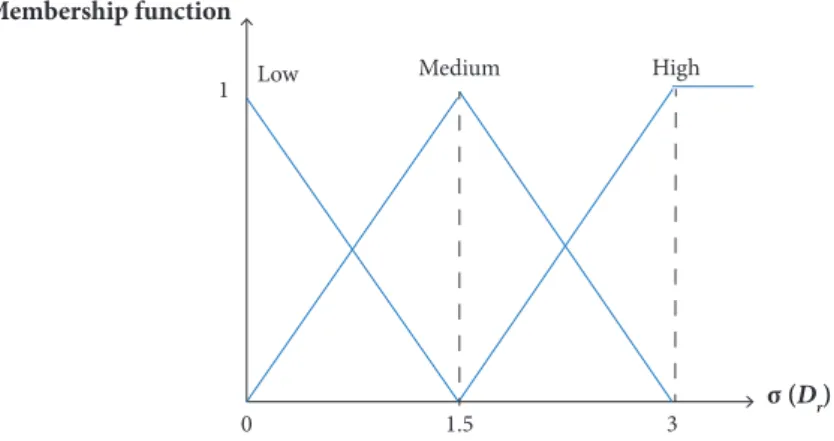
The membership functions of the mean and standard deviation values are shown in Figs. 11 and 12, respectively. The fuzzy rule set for drag is:
1. If μD is very high and σD is high then drag preference function is very low (0).
2. If μD is very high and σD is medium then drag preference function is very Low (0).
3. If μD is very high and σD is low then drag preference function is low (0.35).
4. If μD is high and σD is high then drag preference function is very low (0).
5. If μD is high and σD is medium then drag preference function is low (0.35).
F (μ, σ) Fuzzy system
μD
J. Aerosp. Technol. Manag., São José dos Campos, v10, e3618, 2018 A New Approach for Robust Design Optimization Based on the Concepts of Fuzzy Logic and Preference Function
xx/xx 15/22
High Very high
μ (D
r)
Membership function
Medium Low
0 0.5 0.7 1.5
High
σ (D
r)
Membership function
Medium Low
0 1.5
1
3
F (w) Fuzzy system
w
Figure 11. Membership functions of the mean value of normalized drag.
Figure 12. Membership function of the standard deviation of normalized drag.
Figure 13. Fuzzy preference function of weight force. 6. If μD is high and σD is low then drag preference function is medium (0.7).
7. If μD is medium and σD is high then drag preference function is Low (0.35).
8. If μD is medium and σD is medium then drag preference function is medium (0.7).
9. If μD is medium and σD is low then drag preference function is high (1).
10. If μD is low and σD is high then drag preference function is low (0.35).
11. If μD is low and σD is medium then drag preference function is high (1).
12. If μD is low and σD is low then drag preference function is high (1).
Preference Function of Wing Weight
Unlike the drag, uncertainties don’t affect the wing weight, so there is no need to calculate mean and standard deviation in this case. The values of normalized wing weight are as input to the fuzzy system (Fig. 13).
J. Aerosp. Technol. Manag., São José dos Campos, v10, e3618, 2018 Babaei AR; Setayandeh MR
xx/xx 16/22
The fuzzy rule set for wing weight is:
1. If μW is very high then wing weight preference function is very Low (0).
2. If μW is high then wing weight preference function is low (0.35).
3. If μW is medium then wing weight preference function is medium (0.7).
4. If μW is low then wing weight preference function is high (1).
Figure 14. Membership function of normalized wing weight.
High Very high
μ (W
T0)
Membership function
Medium Low
0 1
0.05 0.5 0.7
High Very high
μ (ΔC
L)
Membership function
Medium Low
0 1
0.35 0.7 1.05
Preference Function of Lift Coefficient
Similar to drag force, uncertainties also affect the lift coefficient. Standard deviation and the mean value of ΔCL are inputs to the fuzzy system. Membership functions of the mean and standard deviation, and the rule set are shown in Figs. 15 and 16, respectively. The lift coefficient preference function is similar to Eq. 42.
Figure 15. Membership function of the mean value of normalized lift coefficient.
The lift coefficient preference function is similar to Eq. 42 and the fuzzy rule set for lift coefficient is:
1. If μΔCl is very high and σΔCl is high then lift coefficient preference function is very low (0).
2. If μΔCl is very high and σΔCl is medium then lift coefficient preference function is very low (0).
3. If μΔCl is very high and σΔCl is low then lift coefficient preference function is low (0.35).
4. If μΔCl is high and σΔCl is high then lift coefficient preference function is very low (0).
5. If μΔCl is high and σΔClv is medium then lift coefficient preference function is very low (0).
6. If μΔCl is high and is low then lift coefficient preference function is low (0.35).
J. Aerosp. Technol. Manag., São José dos Campos, v10, e3618, 2018 A New Approach for Robust Design Optimization Based on the Concepts of Fuzzy Logic and Preference Function
xx/xx 17/22
High
σ (ΔC
L)
Membership function
Medium Low
0 1
0.75 1.5
High Very high
μ (ΔV)
Membership function
Medium Low
0 1
0.15 0.3 0.45
8. If μΔCl is medium and σΔCl is medium then lift coefficient preference function is medium (0.7).
9. If μΔCl is medium and σΔCl is low then lift coefficient preference function is medium (0.7).
10. If μΔCl is low and σΔCl is high then lift coefficient preference function is high (1).
11. If μΔCl is low and σΔCl is medium then lift coefficient preference function is high (1).
12. If μΔCl is low and σΔCl is low then lift coefficient preference function is high (1).
Figure 16. Membership function of the standard deviation of normalized lift coefficient.
Figure 17. Membership function of normalized fuel tank volume. Preference Function of Fuel Tank Volume
Like the wing weight, uncertainties don’t affect the fuel tank volume. The process of making preference function for this constraint is similar to Fig. 13 and normalized ΔV is the only input to the fuzzy system. The membership function of normalized fuel tank volume is shown in Fig. 17.
The fuzzy rule set for fuel tank volume is:
1. If μΔV is very high then fuel tank volume preference function is very low (0).
2. If μΔV is high then fuel tank volume preference function is low (0.35).
3. If μΔV is medium then fuel tank volume preference function is medium (0.7).
J. Aerosp. Technol. Manag., São José dos Campos, v10, e3618, 2018 Babaei AR; Setayandeh MR
xx/xx 18/22
OPTIMIZATION ALGORITHM
As mentioned before, the NSGA algorithm is considered as the optimizer. Since the optimization problem is a constrained problem, penalty function method is used for implementation. The specifications of NSGA for optimization in this study are in Table 3.
Table 3. Specifications of NSGA.
Parameter Value
Generation 30
Population size 100
Mutation rate 0.1
Selection rate 0.5
DESIGN OPTIMIZATION RESULTS
As already mentioned, two design optimizations have been done in this paper that includes: deterministic optimization, and robust optimization. It was also stated that the utopian distance concept is used for final solution selection so the utopian values of wing drag and weight must be calculated at first. From a single objective optimization, utopian values of drag and weight and their specifications were obtained as follows (Tables 4 and 5):
Table 4. Utopian values for drag.
Cr (m) b (m) Λ0.5 (deg) Dut (N)
15.29 57.17 41.83 49910
Table 5. Utopian values for weight.
Cr (m) b (m) Λ0.5 (deg) Wut (N)
15.42 56.16 40.68 6.0631 × 10⁵
Four optimal solutions (Pareto frontier) were achieved for deterministic optimization, presented in Table 6. It is worth noting that the details of deterministic optimization are available in Babaei et al. (2015).
Table 6. Results of deterministic optimization.
Pareto point Cr(m) b (m) Λ0.5(deg) Dut (N)
1 14.92 58.6 39.2 0.83
2 15.77 55.29 38.7 0.76
3 14.8 59.2 38 0.86
4 15.4 57.5 41.3 0.73
As already noted, each point that has lower distance is the best solution among Pareto frontier. So for deterministic optimization, number four has lower distance and is the final solution. The full specifications of this point are given in Table 7.
Table 7. The full specification of final solution.
Cr (m) b (m) Λ0.5 (deg) S (m
2) AR C
L V (m
3) W (N) D (N)