UM MODELO ESTATÍSTICO MULTIVARIADO
PARA PREVER O COMPORTAMENTO DE
GEÓRGIA PENIDO SAFE
UM MODELO ESTATÍSTICO MULTIVARIADO
PARA PREVER O COMPORTAMENTO DE
HEURÍSTICAS EM VERIFICAÇÃO FORMAL
Tese apresentada ao Programa de Pós--Graduação em Ciência da Computaão do Instituto de Ciências Exatas da Universi-dade Federal de Minas Gerais como req-uisito parcial para a obtenção do grau de Doutor em Ciência da Computaão.
Orientador: Claudionor Nunes Coelho Jr
Belo Horizonte
GEÓRGIA PENIDO SAFE
A MULTIVARIATE CALIBRATION MODEL
TO PREDICT FASTER
FORMAL VERIFICATION HEURISTICS
Thesis presented to the Graduate Program in Computer Science of the Federal Univer-sity of Minas Gerais in partial fulfillment of the requirements for the degree of Doctor in Computer Science.
Advisor: Claudionor Nunes Coelho Jr
Belo Horizonte
c
2011, Geórgia Penido Safe. Todos os direitos reservados.
Safe, Geórgia Penido
S128m A multivariate calibration model to predict faster formal verification heuristics / Geórgia Penido Safe. — Belo Horizonte, 2011
xxiv, 108 f. : il. ; 29cm
Tese (doutorado) — Federal University of Minas Gerais
Orientador: Claudionor Nunes Coelho Jr
1. Computaão Teses. 2. Programaão paralela -Teses. 3. Verificaão funcional - -Teses. I. Titulo.
To my parents, Jose Luciano and Glete,
For teaching me what really matters
To my husband and my daughter, Gustavo and Lavinia, For being the reason of everything
Acknowledgments
First of all, I would like to thank God for all He has given me. Without Him, none of this would have been possible.
Thanks to my supervisor, who was always beside me giving all his support and friendship. I will never forget.
Thanks to all my family: my husband and Lavinia for the comprehension and support, my parents for the sincere opinions, my sister Erika for trying to help, my sister Andresa and my brother Luciano, for the good wishes.
Thanks to Professor Luis Filipe, for helping with all his experience in the paper elaboration.
It is a pleasure for me to work with all the wonderful people from Jasper. Thanks to all of you for every smile I received when my paper was accepted and for all support. Thanks to Celina, for helping in the data collection.
Thanks to Jose Nacif, for the discussions, support and useful hints.
Thanks to Renata, for the patience and guiding in all university processes. People like you make our department one of the best in our country.
Thanks to all professors that I consider my friends: José Marcos, Antônio Otávio and Antônio Alfredo, for being part of all this.
Thanks for the examinators, for the valuable ideas and corrections.
Resumo
Verificação funcional é “o” principal gargalo na produtividade de empresas desenvolve-doras de chips. Como a verificação funcional é um problema NP-completo, ela depende de um grande número de heurísticas e seus parâmetros de configuração (“resolvedores"). Normalmente o número de resolvedores disponíveis excede em muito o poder de proces-samento disponível. Com o advento da programação paralela, a verificação funcional pode ser otimizada através da seleção dos melhores n resolvedores para rodar em par-alelo, aumentando assim a chance de se alcançar o término da verificação. Este trabalho apresenta um modelo estatístico baseado em métricas estruturais para construir esti-madores de tempo de verificação para os resolvedores, permitindo então a seleção dos
n melhores resolvedores para rodar em paralelo. Esta metodologia considera tanto o tempo de execução estimado dos resolvedores quanto a correlação entre estes re-solvedores. Resultados confirmaram que a metodologia pode ser um mecanismo muito rápido e eficaz para a seleção dos melhores resolvedores, aumentando a chance de se resolver o problema.
Abstract
Functional verification is “the” major design-phase bottleneck for silicon productivity. Since functional verification is an NP-complete problem, it relies on a large number of heuristics with associated parameters (engines). With the advent of parallel pro-cessing, formal verification can be optimized by selecting the best n engines to run in parallel, increasing the chance of reaching verification successful termination. In this work, we present an statistical model to build engine estimators based on structural metrics and to select n engines to run in parallel. The methodology considers both engines’ estimated performance and engines’ correlation. Results confirmed that the methodology can be a very quick selection mechanism for parallelization of engines in order to increase the chance of running the best engines to solve the problem.
List of Figures
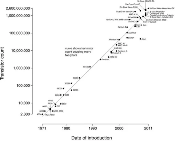
1.1 Transistor counts for integrated circuits plotted against their dates of
intro-duction. . . 2
1.2 The verification gap leaves design potential unrealized. . . 3
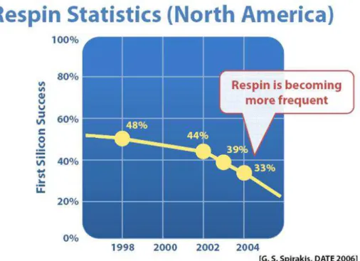
1.3 Re-spin frequency in North America, as brought by Fujita Lab. . . 3
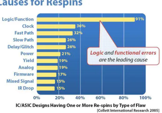
1.4 Re-spin causes in North America, as brought by Fujita Lab. . . 4
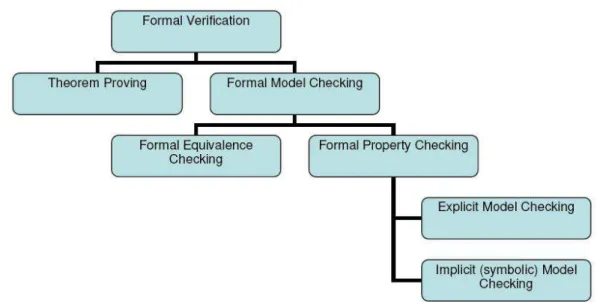
2.1 Formal verification classification overview. . . 14
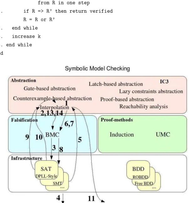
2.2 Symbolic model checking techniques overview. . . 16
2.3 Decision tree diagram. . . 17
2.4 Reductions: merge duplicates and eliminate redundancy. . . 18
2.5 Final BDD. . . 18
2.6 Graphical visualization of k-induction algorithm. . . 25
2.7 Graphical visualization of CEX-based abstraction algorithm. . . 29
2.8 Graphical visualization of Proof-based abstraction algorithm. . . 31
2.9 Graphical visualization of interpolation algorithm. . . 33
3.1 Globally linear nature of linear regression. . . 40
3.2 1-NN and 5-NN neighborhood. . . 42
3.3 Locally constant nature of kNN regression. . . 44
3.4 Basic principle of PCA in two dimensional case. . . 45
4.1 The investor‘s opportunity set. . . 48
4.2 Indifference curves. . . 49
4.3 Investor equilibrium. . . 51
4.4 Investor’s opportunity set with several alternatives. . . 52
4.5 Risk and return possibilities for various assets and portfolios. . . 59
4.6 The efficient frontier. . . 60
4.7 Combinations of the riskless asset in a risky portfolio. . . 60
5.1 Methodology to identify variables with polynomial effect over an engine. . 74
6.1 Polinomial effect for smaller values versus exponential effect for larger values. 84 6.2 Results comparison for selection heuristics. . . 88
A.1 SCOAP controllability equations. . . 103
A.2 SCOAP observability equations. . . 104
A.3 Flip-flop. . . 104
A.4 SCOAP observability equations. . . 105
List of Tables
3.1 Main differences between linear and k-nearest neighbors methods. . . 44
4.1 Frequency function. . . 53
5.1 Symbols convention. . . 68
5.2 r-squared for engine estimators with all data. . . 76
6.1 Percentage of times smaller distance matched correctly for each group at the end of validation process. . . 85
6.2 Percentage of time of each kind of match for selection based in execution time. . . 86
6.3 Percentage of time of each kind of match for selection based in execution time and variance. . . 87
6.4 Mean r-squared for engine estimators after cross-validation. . . 88
Contents
Acknowledgments xi
Resumo xiii
Abstract xv
List of Figures xvii
List of Tables xix
1 Introduction 1
1.1 Motivation and Goal . . . 1
1.2 Problem Definition . . . 5
1.3 Related work . . . 8
1.4 Summary of the thesis . . . 9
1.4.1 Chapter 2 . . . 9
1.4.2 Chapter 3 . . . 10
1.4.3 Chapter 4 . . . 10
1.4.4 Chapter 5 . . . 10
1.4.5 Chapter 6 . . . 11
1.4.6 Chapter 7 . . . 11
1.4.7 Appendix 1 . . . 11
1.5 Thesis contributions . . . 11
2 Formal Verification 13 2.1 Theorem proving . . . 13
2.2 Formal model checking . . . 14
2.2.1 Formal equivalence checking . . . 14
2.2.2 Formal property checking . . . 15
2.3 Symbolic Model Checking . . . 15 2.3.1 Infrastructure Layer . . . 16 2.3.2 Falsification and Proof Methods Layer . . . 23 2.3.3 Abstraction Layer . . . 27 2.3.4 Proof engines . . . 33
3 Statistical Learning 35
3.1 Multivariate regression . . . 36 3.2 Linear regression . . . 37 3.3 Nearest neighbor method . . . 40 3.4 Principal component analysis . . . 43
4 Mean Variance Portfolio Theory 47
4.1 The Opportunity Set . . . 47 4.2 The Indifference Curves . . . 49 4.3 Opportunity Set Under Risk . . . 51 4.3.1 Return Distribution . . . 52 4.3.2 Variance . . . 53 4.4 Combination of Assets . . . 54 4.5 Efficient Frontier . . . 58
5 A Multivariate Calibration Model to Predict Faster Verification
Heuristics 67
5.1 Independent Variables (~x) . . . 68 5.2 Data set . . . 71 5.2.1 Data set partition . . . 71 5.3 Engine Estimators . . . 72 5.3.1 Linearization of Exponential Equations . . . 72 5.3.2 Polynomial Effect of Variables . . . 73 5.3.3 Multivariate regression . . . 75 5.4 Engines’ selection mechanisms . . . 77 5.4.1 Maximizing Performance . . . 78 5.4.2 Minimizing Correlation . . . 78 5.4.3 Maximizing Performance and Chance of Success . . . 79
6 Results 83
6.1 Multivariate regression . . . 83 6.2 Smallest distances . . . 84
6.3 Selection based on engine’s time . . . 85 6.4 Selection based on engine’s time and correlation . . . 86 6.5 Summarization . . . 87
7 Conclusions 89
Bibliography 93
A Testability measures 101
A.1 SCOAP (Sandia Controllability Observability Analysis) [42] . . . 102 A.2 COP (Controllability/Observability Program) [18] . . . 105 A.3 PREDICT [72] . . . 105 A.4 VICTOR [69] . . . 106 A.5 STAFAN (Statistical Fault Analysis) [52] . . . 106 A.6 TMEAS (Testability Measure Program) [43] . . . 106 A.7 CAMELOT (Computer-Aided Measure for Logic Testability) [13] . . . 108
Chapter 1
Introduction
1.1
Motivation and Goal
Electronic designs have been growing rapidly in both device count and functionality, concretizing Moore’s Law, as it can be seen in figure 1.1.
This growth has been enabled by deep sub-micron fabrication technology, and fueled by expanding consumer electronics, communications and computing markets. A major impact on the profitability of electronic designs is the increasing productivity gap. That is, what can be designed is lagging behind what silicon is capable of delivering [78], as shown in figure 1.2 [11].
Functional verification is already “the” major design-phase bottleneck, and it will only get worse with the bigger capacities on the horizon [50].
Broadly speaking, the verification crises can be attributed to the following inter-acting situations [78]:
• Verification complexity grows super-linearly with design size,
• The increased use of software, which has intrinsically higher verification complex-ity,
• Shortened time-to-market,
• Higher cost of failure (low profit margin).
A consequence of this verification crisis is that re-spins are becoming more fre-quent, as it can be seen in figure 1.3, and the main causes are logic and functional errors, as shown by statistics in figure 1.4. These errors could be reduced by a better functional verification.
2 Chapter 1. Introduction
Figure 1.1. Transistor counts for integrated circuits plotted against their dates of introduction.
Automated formal verification arrived to aid. Allowing the exhaustive exploration of all possible behaviors, automated formal verification is easy to use and increases the reliability of the design.
Despite all the recent advances in formal verification technology [33], formal veri-fication is an NP-complete problem in the size of the trace description (Binary Decision Diagrams state-explosion problem) and in the verification time (SAT solvers). There-fore, as many other NP-complete problems, practical solutions implement heuristics to try to solve efficiently such problems.
1.1. Motivation and Goal 3
Figure 1.2. The verification gap leaves design potential unrealized.
Figure 1.3. Re-spin frequency in North America, as brought by Fujita Lab.
best engines will speed up the verification process and increase the chance of successful termination. However, selecting the best heuristics and parameters to prove a property is a complex problem.
4 Chapter 1. Introduction
Figure 1.4. Re-spin causes in North America, as brought by Fujita Lab.
for each available engine and gets the first result available. However, since engines and associated parameters may be much more numerous than the processing power avail-able, this approach can easily be shown not to scale. On the other hand, verification engineers may have a feeling of the best heuristic to prove a property, but with the increase in design size, trusting in these feelings becomes a big risk.
With the advent of parallel processing (simultaneous use of more than one CPU or processor core to execute a program or multiple computational threads), the possibility of running multiple processes in parallel became more transparent and viable. As a consequence, relying on the use of multiple processes/threads in order to get the best results arose as a way to improve formal verification.
In general, there are a large pool of engines, but only a small number of process-ing cores. The problem then becomes selectprocess-ing the best subset of engines that will increase the chance of solving the problem, which in this context means reaching a proof conclusion.
The goal of this work is to generate a forecasting mechanism to classify and select the n best engines to run in parallel, in order to maximize the chance of proof conclusion or successful termination.
cir-1.2. Problem Definition 5
cuits, given the verification crisis and the existence of so many different engines to implement formal verification.
In a verification tool that implements several formal verification heuristics with associated parameters, selecting the best heuristics and parameters to prove a property becomes a complex problem.
We know that designs are getting bigger and bigger and that time to verify systems is crucial to improve their time-to-market. Therefore, choosing engines with greater chance of solving the problem turns out to be an important question.
1.2
Problem Definition
A Hardware Description Language (HDL) is a standard text-based expression of the temporal behavior and/or (spatial) circuit structure of an electronic system. The vast majority of modern digital circuit-design revolves around an HDL-description of the desired circuit, device, or subsystem, with VHDL (VHSIC Hardware Description Lan-guage) and Verilog HDL being the two dominant HDLs. SystemVerilog is a combined HDL and Hardware Verification Language (HVL) based on extensions to Verilog.
A simple example of two flip-flops swapping values every clock in Verilog is:
module toplevel(clock,reset); input clock;
input reset;
reg flop1; reg flop2;
always @ (posedge reset or posedge clock) if (reset)
begin
flop1 <= 0; flop2 <= 1; end
else begin
6 Chapter 1. Introduction
endmodule
Property checking takes a design and a property which is a partial specification of the design and its surroundings, and proves or disproves that the design satisfies the property. A property is essentially an abstracted description of the design, and it acts to confirm the design through redundancy.
Properties may be specified in many ways. A Hardware Verification Language, or HVL, is a programming language used to verify the designs of electronic circuits written in a hardware description language. OpenVera [6], Specman(e) [3], and SystemC [5] are the most commonly used HVLs. SystemVerilog [1] attempts to combine HDL and HVL constructs into a single standard. Open Verification Library (OVL) [2] is a library of property checkers for digital circuit descriptions written in popular HDLs. Property Specification Language (PSL) [4] is a language developed by Accellera for specifying properties or assertions about hardware designs.
SystemVerilog, for example, supports assertions, assumptions and coverage of properties. An assertion specifies a property that must be proven true. An assumption establishes a condition that a formal logic proving tool must assume to be true. In simulation, both assertions and assumptions are verified against test stimulus. Prop-erty coverage allows the verification engineer to verify that assertions are accurately monitoring the design.
A SystemVerilog assertion example is:
property req_gnt; @(posedge clk) req |=> gnt; endproperty
assert_req_gnt: assert property (req_gnt)
else $error("req not followed by gnt.");
1.2. Problem Definition 7
A program that checks a property is also called a model checker, referring the design as a computational model of a real circuit.
The idea behind property checking is to search the entire state space for points that fail the property. If such a point is found, the property fails and the point is a counterexample. Next, a waveform derived from the counterexample is generated, and the user debugs the failure. Otherwise, the property is satisfied.
What makes property checking a success in industry are efficient SAT solvers or symbolic traversal algorithms that enumerate the state space implicitly (see chapter 3).
Each group of heuristics and algorithms (with its set of configuration parameters) used to accomplish one proof can generate a different engine e (or solver).
Some parameter examples from the SAT-solving world include decision variable and phase selection, clause deletion and initial variable ordering. The complex ef-fects and iterations between these parameters render the design and implementation of a high-performance decision procedure (or, indeed, a high-performance heuristic algorithm for any NP-hard problem) so challenging that in many ways the process resembles an art rather than a science [51].
The behavior and performance of each engine is highly dependent on circuit design, or the property to be proved, whose behavior can be characterized by a set of independent variables ~x and a set of unknown variables U~. We consider U~ to be insignificant in the problem context. However, since the problem is hard, we will always have a chance that the chosen independent variables won’t be enough to explain the behavior of a given verification problem instance.
Some independent variables examples are the number of flip-flop bits and the number of counter bits in the design.
Given
• a design and a property to be proved expressed by vector~xof selected independent variables that are supposed to explain the behavior of the verification problem,
• N proof heuristicsE1, E2, ...EN, each one configurable by vectorp~i of parameters,
naming engines e1, e2, ...eN,
the objective of this work is to statistically compute engines estimators
• e˜i(~x)∝ei
8 Chapter 1. Introduction
1. n < N
2. e1, ...,en is the n set of engines with the biggest chance of reaching to a proof
conclusion.
where function ˜ei(~x) returns the estimated time of engine i to prove a property
whose design is characterized by independent variables ~x. In fact, the estimated ex-ecution time of engine i is a function of ~x and U~, where U~ refers to some unknown variables. As already stated, we approximate ˜e(~x, ~U) as e˜(~x). This approximation is valid if the error introduced by droppingU~ is small.
1.3
Related work
Traditionally, formal verification has employed engines based on SAT and BDD al-gorithms. Such algorithms have been constructed with several heuristics, captured by parameters (MiniSAT [28], Cudd [76], GRASP [55], zchaff [81], SATO [79], Berk-Min [30]). However, these engines are usually executed in a monolithic way, i.e. with no or with few parameters, with exception of the work [51], which tunes the heuristics parameters. Besides that, there are many algorithms employed in formal verification (such as reachability analysis, induction, bounded model checking and proof-based abstraction), each of them with its limitations and advantages, depending on the ap-plications.
McMillan et al. works [8; 9; 60; 58] compare many model checking techniques on a set of benchmark model checking problems derived from microprocessor verification. As it can be seen, performance of each technique depends greatly on circuit design, which generates different Conjunctive Normal Form (CNF) representations that may be best solved by different approaches.
Automatic parameterization of formal verification engines has only attracted at-tention recently. The closest work is [51], which presents a methodology to tune heuris-tic parameters, improving a specific heurisheuris-tic performance. They employed ParamILS, a parameter optimization tool, to enhance SPEAR, a high-performance modular arith-metic decision procedure and SAT solver. Results show speedups between 4.5 and 500 in comparison to a manually-tuned version of SPEAR that already reached the performance of a state-of-the-art SAT solver.
1.4. Summary of the thesis 9
enhancement here is that we deal well with situations where a heuristic may perform well to a design, but very badly to another design (in this case, even with parameter optimization, speed ups can be difficult to reach). Being able to point to an optimal heuristic and parameter configuration among all available ones is a great step in the verification process.
In the area of semiconductor manufacturing, increased yield and improved prod-uct quality result from reducing the amount of wafers produced under suboptimal operating conditions. Some works employing multivariate statistical process control (MSPC) in the semiconductor manufacturing process in order to improve fault de-tection have been found. As examples, [22] presents a complete MSPC application method that combines recent contributions to the field, including multiway principal component analysis (PCA), recursive PCA, fault detection using a combined index, and fault contributions from Hotelling’s T2 statistic. [67] presents an enhancement to
previous work that consisted of a fault detection method using the k-nearest-neighbor rule (FD-kNN). To reduce memory requirements and computation time of the proposed FD-kNN method while still keeping its advantage of handling nonlinear and multimode data, an improved FD-kNN algorithm based on principal component analysis, denoted as PC-kNN has been proposed.
1.4
Summary of the thesis
1.4.1
Chapter 2
Chapter 2 presents a global review on Formal Verification and a detailed review on Symbolic Model Checking, pointing the most used algorithms and heuristics.
The main goal is to explain some of the main model checking heuristics, em-phasizing the fact that one heuristic can have many variations, controlled by their configuration parameters. The parameters direct the heuristics in the decisions to take.These decisions bring up different behaviors, which can improve performance for some designs, but not for others. The existence of a large number of engines due to the large number of heuristics and their variations (parameters) and the fact that heuristics can be good for one design, but bad for another, is one of the justifications to apply the proposed methodology: choose the engines with the biggest chance of success to prove a property.
10 Chapter 1. Introduction
1.4.2
Chapter 3
Chapter 3 presents a review on Statistical Learning techniques, detailing methods that can be used to build prediction models in a multivariate scenario.
In order to choose the n engines with the best chance of success, it is mandatory to have a time prediction model for each engine, since the main aspect of the engine performance is its execution time. We can consider that the most efficient engines have smaller execution times (independently of the proof result: proven or falsified), and good engine execution time estimators will influence in the quality of this work.
A property to be proven will be expressed by a set of independent variables, that are comprised by metrics gotten from the design. Therefore, a multivariate linear regression model will be used to generate the engine estimators.
The main goal is to explain the statistical theory upon which the engine estimators have been generated.
1.4.3
Chapter 4
Chapter 4, Mean Variance Portfolio Theory, presents an interesting finance theory which will be applied in our solution.
Choosing engines by their performance (execution times) seems to be a good methodology, but the correlation between engines is also a factor that needs to be taken into account. Correlated engines tend to have similar behaviors and all selected correlated engines could lead to the same final result: if they all have longer execution time, we could arrive to no proof conclusion. In order to maximize the chance of suc-cess, the proposed solution will try to maximize performance and minimize correlation between selected engines.
This chapter explains the Mean Variance Portfolio Theory and their formulas that will be applied in our solution.
1.4.4
Chapter 5
Chapter 5 presents designed solution to solve problem defined.
1.5. Thesis contributions 11
1.4.5
Chapter 6
Chapter 6 presents experimental results.
Two solutions were tested: (1) maximize performance and (2) maximize perfor-mance and minimize correlation. Both methodologies proved to be efficient, with speed ups of more than 3 times compared to a not optimal selection of engines.
1.4.6
Chapter 7
Chapter 7 concludes the work, presenting possible future works.
1.4.7
Appendix 1
Appendix 1 presents some testability measures that can be used as input data to the predictor.
1.5
Thesis contributions
This work’s contributions are:
• Statistical model to predict faster proof heuristics
A model will be proposed to predict faster proof engines (heuristics with asso-ciated parameters), given a design and a property to be proved. Multivariate statistics techniques will be used to generate this prediction model.
• Analysis of variable effect
Although variables seem to have an exponential effect over the prediction model due to inheritance of NP-completeness of the verification process, heuristics can be affected in different ways by the metrics collected from the design and the property to be proven. It is possible, for example, to have a metric that has an exponential effect on one heuristic, while having a polynomial effect on another heuristic. This work tries to identify polynomial effects of variables through the analysis of the prediction model error.
• Analysis of engine correlation
Chapter 2
Formal Verification
Verification importance has emerged as an indispensable phase of digital hardware design development process. The increasingly competitive market makes cost of chip failure enormous, forcing traditional “black-box” verification methodology to give place to a “white-box” methodology.
In order to accomplish verification of designs that get more and more complex, traditional simulation faces the drawback that every time more simulation cases are necessary to arrive to accepted coverage levels. In addition, the increase of simulation sequences, the test-benches, makes verification process longer and more difficult, con-sidering the effort to debug the test-benches, what may require the understanding of design characteristics, the features being tested and the simulation results.
Formal verification comes to solve this gap between design complexity and veri-fication efforts.
Formal verification ensures that a design is correct with respect to a property that can be proved. The correctness of a property is based on its specification. Mathematical methods are used to prove or disprove a property.
Formal verification can be broadly classified as shown in Figure 2.1. This chapter gives a high level view of formal verification and a detailed view of Symbolic Model Checking.
2.1
Theorem proving
One of the earliest approaches to formal verification was to describe both the imple-mentation and the specification in a formal logic. The correctness was then obtained by, in the logic, proving that the specification and the implementation were suitably related [17].
14 Chapter 2. Formal Verification
Figure 2.1. Formal verification classification overview.
Unfortunately, theorem proving technique requires a large amount of effort by the user developing specifications of each component and in guiding the theorem proving user through all the lemmas.
2.2
Formal model checking
Formal model checking [17] consists of a systematic exhaustive exploration of all states and transitions in a model.
Model checking tools face an exponential blow up of the number of state elements (e.g. registers, latches), commonly known as the state explosion problem, which must be addressed to solve most real-world problems.
Model checking is largely automatic, being the most successful approach to formal verification in use today. Model checking tools are typically classified as equivalence checking or property checking.
2.2.1
Formal equivalence checking
2.3. Symbolic Model Checking 15
2.2.2
Formal property checking
In formal property checking, properties describing the desirable/undesirable features of the design are specified using some formal logic (e.g. temporal logic) and verification is performed by proving or disproving that the property is satisfied by the model.
This work concentrates on efficient property checking techniques that make formal verification practical and realizable.
Model checking approaches are broadly classified into two types, based on state enumerations techniques employed: explicit and implicit (or symbolic).
• Explicit
Explicit model checking techniques [49] store the explored states in a large hash table, where each entry corresponds to a single system state. A system with as few as hundreds state elements amounts to a state space with 1011 states, arriving easily to the state explosion problem.
• Implicit (symbolic)
Symbolic model checking techniques [57] stores sets of explored states symboli-cally by using characteristics functions represented by canonical/semi-canonical structures, and traverse the state space symbolically by exploring a set of states in a single operation.
Symbolic model checking will be largely explored in the next section.
2.3
Symbolic Model Checking
Symbolic model checking is a method to prove properties about finite transition sys-tems, using symbolic state enumeration. The properties are usually in one of the different flavors of temporal logic formulas such as Linear Time Logic (LTL) [66] or Computational Tree Logic (CTL) [12; 23].
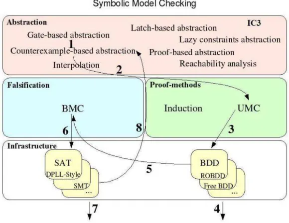
According to Figure 2.2, this section will cover model checking techniques based on three main tasks [34]: finding counter-examples or bugs (Falsification layer), proving the correctness of the specification (Proof Methods layer) and obtaining smaller models that make verification possible (Abstraction layer). Prior to that, basic infrastructure required to build scalable verification algorithms are presented (Infrastructure layer).
16 Chapter 2. Formal Verification
Figure 2.2. Symbolic model checking techniques overview.
2.3.1
Infrastructure Layer
Canonical structures as Binary Decision Diagrams (BDDs) [7; 19] allow constant time satisfiability checks of Boolean expressions and are used to perform symbolic Boolean function manipulations [7; 77]. Although BDD-based methods have greatly improved scalability in comparison to explicit state enumeration techniques, they are still limited to designs with a few hundred state holding elements.
2.3. Symbolic Model Checking 17
2.3.1.1 Binary Decision Diagrams (BDDs)
A BDD is just a data structure for representing a Boolean function. Bryant [19] introduced the BDD in its current form, although the general ideas have been around for quite some time.
A BDD is a directed acyclic graph in which each vertex is labeled by a Boolean variable and has outgoing arcs labeled as “then” and “else” branches. The value of the function for a given assignment to the inputs is determined by traversing from the root down to a terminal label, each time following the then (else) branch corresponding to the value 1 (0) assigned to the variable specified by the vertex label. The value of the function then equals the terminal value.
In an ordered BDD, all vertex labels must occur according to a total ordering of the variables. In a reduced ordered BDD (ROBDD), besides the ordering criteria, two more conditions are imposed:
1. two nodes with isomorphic BDDs are merged, and
2. any node with identical children is removed.
These conditions make a reduced ordered BDD a canonical representation for Boolean functions. In the sequel, BDD will refer to ROBDD.
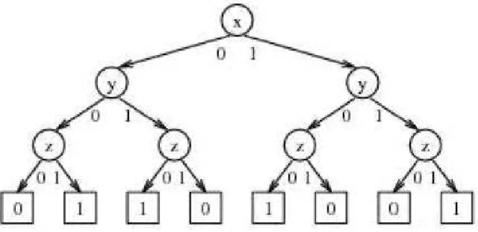
Conceptually, we can construct the BDD for a Boolean function as follows. First build a decision tree for the desired function, obeying the restrictions that along any path from root to leaf, no variable appears more than once, and that along every path from root to leaf, the variables always appear in the same order, as it can be seen in Figure 2.3.
18 Chapter 2. Formal Verification
Next, apply the following two reduction rules as much as possible: (1) merge any duplicate (same value and same children) nodes, and (2) if both child pointers of a node point to the same child, delete the node because it is redundant, as it can be seen in Figure 2.4.
Figure 2.4. Reductions: merge duplicates and eliminate redundancy.
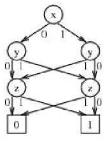
The resulting directed, acyclic graph, presented in Figure 2.5, is the BDD for the function.
Figure 2.5. Final BDD.
In practice, BDDs are generated and manipulated in the fully reduced form, without ever building the decision tree. In a typical implementation, all BDDs in use by an application are merged as much as possible to maximize node sharing, so a function is represented by a pointer to its root node.
2.3. Symbolic Model Checking 19
Choosing a good variable order is important. In general, the choice of variable order can make the difference between a linear size BDD and an exponential one.
Researchers have developed several heuristics to obtain a good variable ordering that produce compact BDD representation [10; 31; 71]. Even though finding a good BDD variable ordering is not easy [16], for some functions such as integer multiplication, there does not exist an ordering that gives a sub-exponential size representation [20].
The primary limitation of the BDD-based approaches is the scalability, i.e., BDDs constructed in the course of verification often grow extremely large, resulting in space-outs or severe performance degradation due to the paging [68]. Moreover, BDDs are not very good representations of state sets, especially when the sharing of the nodes is limited. Choosing a right variable ordering for obtaining compact BDDs is very important. Finding a good ordering is often time consuming and/or requires good design insight, which is not always feasible. Several variations of BDDs such as Free BDDs [48], zBDDs [61], partitioned-BDDs [64] and subset-BDDs [70] have also been proposed to target domain specific application; however, in practice, they have not scaled adequately for industry applications. Therefore, BDD-based approaches are limited to designs of the order of a few hundred state holding elements; this is not even at the level of an individual designer subsystem.
2.3.1.2 Boolean Satisfiability (SAT)
The Boolean Satisfiability (SAT) problem is a well-known constraint satisfaction prob-lem, with many applications in the fields of VLSI Computer-Aided Design (CAD) and Artificial Intelligence. Given a propositional formula, the Boolean Satisfiability problem is to determine, whether there exists a variable assignment under which the formula evaluates to true, or to prove that no such assignment exists. The SAT prob-lem is known to be NP-Complete [40]. In practice, there has been tremendous progress in SAT solver technology over the years, summarized in a survey [82].
Most SAT solvers use a Conjunctive Normal Form (CNF) representation of the Boolean formula. In CNF, the formula is represented as a conjunction of clauses, each clause is a disjunction of literals, and a literal is a variable or its negation. Note that in order for the CNF formula to be satisfied, each clause must also be satisfied, i.e., at least one literal in the clause has to be true. Converting a (gate-level) netlist to a CNF formula is straightforward: each gate translates to a set of at most three clauses. For example, an AND gate a =b&c defines the relation a => b&c and b&c=> a, which gives the clauses (!a+b), (!a+c) and (a+!b+!c).
20 Chapter 2. Formal Verification
algorithm iteratively selects variables to resolve until no more variables are left (the problem is satisfiable) or a conflict is encountered (the problem is unsatisfiable). This is equivalent to the existential quantification of variables, and is exponential in memory usage.
Later, Davis, Longemann and Loveland [26] proposed a Depth-First Search (DFS)-based algorithm with backtracks. For historical reasons it is also known as the Davis-Putnam-Longemann-Loveland (DPLL) algorithm. Most modern high-performance SAT solvers are based on a DPLL-style procedure.
A typical SAT solver relies on a few key procedures:
• Decides: makes a decision by picking an unassigned variable and assigning it a value (0 or 1). It returns false if there are no more unassigned variables.
• Deduces: propagates the decision assignment and assignments implied by prop-agation in the clauses. It returns false if these assignments conflict.
• Analyses: determines, when a conflict occurs, which decision to backtrack. Op-tionally it learns new information from the conflict.
• Backtrack: undoes assignments up to a specified decision level. A new assignment is made to branch the search.
Algorithm below shows how these procedures work together.
SAT() {
Dlevel = 0; While (true) {
If (deduce() == false) { Dlevel = analyse();
If (dlevel == 0) return UNSAT; Else backtrack(dlevel);
}
Else if (decide() == false) return SAT; Else dlevel = dlevel + 1;
} }
2.3. Symbolic Model Checking 21
for improvement. The order in which a variable is picked, and the value assigned in the decision, can affect the actual space. The same is true with conflict analysis and backtracking. Backtracks can be made non-chronologically (that is, not just backtrack to the last decision) with an intelligent analysis of the conflict. Also, the efficient im-plementation of the heavily used deduction/propagation procedure can greatly improve the overall performance of the algorithm.
Examples of SAT solvers are CHAFF [62], GRASP [74] and SATO [80].
Algorithm advances are the key to the success of SAT-based formal methods. Some of the most promising results on certain problem instances that involve low overhead will be now mentioned.
Frequent restarts The state-of-the-art SAT solvers also employ a technique called random restart [62] for greater robustness. The first few decisions are very im-portant in the SAT solver. A bad choice could make it very hard for the solver to exit a local non-useful search space. Since it is very hard to decide a priori what a good choice might be for decisions, the restart mechanism periodically undoes all decisions and starts afresh. The learned clauses are preserved between restarts; therefore, the search conducted in previous rounds is not lost. By utilizing such randomizations, a SAT solver can minimize local fruitless search.
Non-conflict-driven Back-jumping This refers to a back-jump to an earlier de-cision level (not necessarily to level 0), without detecting a conflict [65]. It is a variation of frequent restarts strategy, but guided by the number of conflict-driven backtracks seen so far. The goal is to quickly get out of a “local conflict zone” when the number of backtracks occurring between two decision levels ex-ceeds a certain threshold. For hard problem instances, such strategy has shown promising results.
Frequent Clause Deletion Conflict-driven learned clauses are redundant, and therefore, deleting them does not affect satisfiability of the problem. Con-flict clauses, though useful can become an overhead especially due to increased Boolean Constraint Propagation (BCP) time and due to large memory usage. Such clauses can be deleted based on their relevance metric [62] which is com-puted based on number of unassigned literals. One can also compute relevance of a clause based on its frequent involvement in conflict [41].
22 Chapter 2. Formal Verification
a sufficient subset of the literals required to generate the conflict [63]. Using the conflict literals as decision variables, one applies BCP and stops as soon as a conflict is detected. In many cases, fewer literals in the conflict clause are involved.
Early Conflict Detection in Implication Queue The implication queue (in lazy assignment) stores the newly implied variables during BCP. If a newly implied variable is already in the queue with an opposite implied value, conflict can be detected early without doing BCP further [14].
Shorter Reasons First Several unit clauses can imply the same value on a variable at a given decision level. With an intuition that shorter unit clauses decrease the size of implication graph, and hence, the size of conflict clauses, the implications due to shorter clauses are given preference [14].
Satisfiability Modulo Theory (SMT) An SMT instance is a generalization of a Boolean SAT instance in which various sets of variables are replaced by pred-icates from a variety of underlying theories. Obviously, SMT formulas provide much richer modeling language than is possible with Boolean SAT formulas. For example, an SMT formula allow us to model the data path operations of a mi-croprocessor at the word rather than the bit level.
Formally speaking, an SMT instance is a formula in quantifier-free first-order logic, and SMT is the problem of determining whether such formula is satisfiable. In other words, imagine an instance of the Boolean satisfiability problem (SAT) in which some of the binary variables are replaced by predicates over a suitable set of non-binary variables. A predicate is basically a binary-valued function of non-binary variables. Example of predicates include linear inequalities (e.g., 3x+2y−z >4) or equalities involving so-called uninterpreted terms and function symbols (e.g., f(f(u, v), v) = f(u, v)where f is some unspecified function of two unspecified arguments). These predicates are classified according to the theory they belong to. For instance, linear inequalities over real variables are evaluated using rules of the theory of linear real arithmetic, whereas predicates involving uninterpreted terms and function symbols are evaluated using rules of the theory of uninterpreted functions with equality (sometimes referred to as the empty theory).
2.3. Symbolic Model Checking 23
replaced by lower-level logic operations on the bits) and passing this formula to a Boolean SAT solver. This approach has its merits: by pre-processing the SMT formula into an equivalent Boolean SAT formula we can use existing Boolean SAT solvers “as-is” and leverage their performance and capacity improvements over time. On the other hand, the loss of the high-level semantics of the under-lying theories means that SAT solver has to work a lot harder than necessary to discover obvious facts (such as x+y =y+x for integer addition). This obser-vation led to the development of a number of SMT solvers that tightly integrate the Boolean reasoning of a DPLL-style search with theory-specific solvers that handle conjunctions (ANDs) of predicates from a given theory.
Dubbed DPLL(T) [39], this architecture gives the responsibility of Boolean rea-soning to the DPLL-based SAT solver which, in turn, interacts with a solver for theory T through a well-defined interface. The theory solver needs only to worry about checking the feasibility of conjunctions of theory predicates passed on to it from SAT solver, as it explores the Boolean search space of the formula. For this integration to work well, however, the theory solver must be able to participate in propagation and conflict analysis.
2.3.2
Falsification and Proof Methods Layer
Falsification and proof methods, as presented in Figure 2.2, are two opposite ap-proaches, to prove that a property holds or does not hold for a model. Falsification methods cannot verify properties, just falsify them.
2.3.2.1 Bounded Model Checking (BMC)
BMC has been gaining ground as a falsification engine, mainly due to its improved scalability compared to other formal techniques.
In BMC, the focus is on finding a counterexample (CEX) - bug, of a bounded length k. For a given design and correctness property, the problem is translated effec-tively to a propositional formula such that the formula is true if and only if a coun-terexample of length k exists [15]. If no such counterexample is found, k is increased. This process terminates when k exceeds the completeness threshold - CT (i.e., k is sufficiently large to ensure that no counterexample exists) - or when SAT procedure exceeds its time or memory bounds.
24 Chapter 2. Formal Verification
and then clauses are build at each time frame for the unrolled circuit and the property to be checked, which is then fed to a SAT-solver.
Many enhancements have been proposed in the last few years to make the stan-dard BMC procedure [15] scale with large industry designs. One key improvement is dynamic circuit simplification [32], performed on the iterative array model of the un-rolled transition relation, where an on-the-fly circuit reduction algorithm is applied not only within a single time frame but also across time frames to reduce the associated Boolean formula. Another enhancement is SAT-based incremental learning, used to improve the overall verification time by re-using the SAT results from the previous runs [32]. Learning can also be accomplished by a lightweight and goal-directed effective BDD-based scheme, where learned clauses generated by BDD-based analysis are added to the SAT solver on-the-fly, to supplement its other learning mechanisms [46]. There are also many heuristics for guiding the SAT search process to improve the performance of the BMC engine.
Even with the many enhancements just mentioned, sometimes the memory lim-itation of a single server, rather than time, can become a bottleneck for doing deeper BMC search on large designs. The main limitation of a standard BMC application is that it can perform search up to a maximum depth allowed by the physical memory on a single server. This limitation stems from the fact that as the search boundk becomes large, the memory requirement due to unrolling of the design also increases. Especially for memory-bound designs, a single server can quickly become a bottleneck in doing deeper search for bugs. Distributing the computing requirements of BMC (memory and time) over a network of workstations can help overcome the memory limitation of a single server, albeit at an increased communication cost [37].
2.3.2.2 Induction
Although BMC can find bugs in larger designs than BDD-based methods, the cor-rectness of a property is guaranteed only for the analysis bound. However, one can augment BMC for performing proofs by induction [73]. A completeness bound has been proposed [15] to provide an inductive proof of correctness for safety properties based on the longest loop-free path between states. Induction with increasing depthk, and restriction to loop-free paths, consists of the following two steps:
2.3. Symbolic Model Checking 25
• k-step Induction: to prove that if the property holds on a k-length path starting from an arbitrary state, then it also holds on all its extensions to a(k+ 1)-length path.
Algorithm below and Figure 2.6 illustrate k-induction.
Procedure k-induction(M, p) 1. initialize k = 0
2. while true do
3. if Base(M, p, k) is SAT 4. then return counterexample
5. else
6. if Step(M, p, k) is UNSAT 7. then return verified 8. k = k + 1
9. end while end
26 Chapter 2. Formal Verification
The restriction to loop-free paths imposes the additional constraints that no two states in the paths are identical. Note that the base case includes use of the initial state constraint, but the inductive step does not. Therefore, the inductive step may include unreachable states also. In practice, this may not allow the induction proof to go through without the use of additional constraints, i.e., stronger induction invariants than the property itself. To shorten the proof length, one can use any circuit constraints known by the designers as inductive invariants.
A set of over-approximate reachable states of the designs can be regarded as pro-viding reachability constraints. These can be used as inductive invariants to strengthen a proof by induction [45]. In principle, any technique can be used to obtain such over-approximate reachability constraints, including information known by the designer.
2.3.2.3 Unbounded Model Checking (UMC)
UMC comprises methods that can prove the correctness of a property on a design as well as find counter-examples for failing properties.
BDD-based model checking tools do not scale well with design complexity and size. SAT-based BMC tools provide faster counter-example checking, but a proof may require unrolling of the transition relation up to the longest loop-free path. Previous approaches to SAT-based unbounded model checking suffer from large time and space requirements for solution enumeration, and hence are not viable.
New efficient and scalable approaches have been created, like the one based on cir-cuit co-factoring for SAT-based quantifier elimination [35], that dramatically reduces the number of required enumeration steps, thereby, significantly improving the per-formance of pre-image and fixed-point computation in SAT-based UMC. The circuit cofactoring method uses Reduced AIG (AND/INVERTER Graph) representation for the state sets as compared to BDDs and CNF representations. The novelty of the method is in the use of circuit co-factoring to capture a large set of states, i.e., several state cubes in each SAT enumeration step, and in the use of circuit graph simplification based on functional hashing to represent the captured states in a compact manner.
2.3. Symbolic Model Checking 27
2.3.3
Abstraction Layer
Obtaining appropriate abstract models that are small and suitable for applying falsifi-cation or proof methods have been the subject of research for quite some time [24; 54]. Abstraction means, in effect, removing information about a system which is not relevant to a property to be verified. In the simplest case, a system can be viewed as a large collection of constraints, and abstraction as removing constraints that are irrelevant. The goal in this case is not so much to eliminate constraints per se, as to eliminate state variables that occur only in irrelevant constraints, and thereby to reduce the size of the state space. A reduction of the state space in turn increases the efficiency of model checking, which is based on exhaustive state space exploration.
Figure 2.2 lists some well known abstractions, which are described below.
2.3.3.1 Gate-based abstraction
Gate-based abstraction is a basic approach to reduce the number of gates to consider during verification. Basically, after a property has been selected to be proved, just the gates that are important to the proof will be considered.
For a signals, representing the property to be proved, just the transitive fanin of signal s should be considered. The transitive fanin of a signals is the set of gates that transitively drives the signals through some other gates (not registers). The transitive fanin arrives to the primary inputs of the circuit that may influence the value of signal
s. The gates in the path from these primary inputs up to signalsare the gates selected by gate-based abstraction approach.
2.3.3.2 Latch-based abstraction
28 Chapter 2. Formal Verification
2.3.3.3 Lazy constraints
Consider a SAT problem is unsatisfiable at a given depthk, i.e., there is no counterex-ample for the safety property at a given depthk. The following partition/classification of the set of latches is valid:
• Propagation latches: for which at least one interface propagation constraint be-longs to set of latch reasons.
• Initial value latches: for which only an initial state constraint belongs to set of latch reasons.
• PPI latches: for which neither the initial constraint, nor any of the interface propagation constraints belongs to set of latch reasons.
Clearly, the set of PPI latches can be abstracted away, since they are not used at all in the proof of unsatisfiability (this has been done in the latch-based abstraction). On the other hand, a propagation latch needs to be retained in the abstract model, since it was used to propagate a latch constraint across time frames for the derived proof. The more interesting case is presented by an initial value latch. It is quite possible that an initial value latch is not really needed to derive unsatisfiability - its initial state constraint may just happen to be used by the SAT solver. It has been observed empirically [34] that on large designs, a significant fraction (as high as 20% in some examples) of the marked latches are initial value latches. Rather than add these latches to an abstract model, the strategy is to guide the SAT solver to find a proof that would not use their initial state values unless needed. This is done by the use of lazy constraints.
A naive way of delaying implications due to initial state constraints is to mark the associated variables, and delay BCP (Boolean Constraint Propagation) on these marked variables during pre-processing. However, this would involve an overhead of checking for such variables during BCP. Rather than change standard BCP proce-dure, the desired effect can be achieved by changing the CNF representation of these constraints. This allows the exploration of the latest improvements in SAT solver technology without modifying the SAT solvers.
2.3.3.4 Counterexample-based abstraction
2.3. Symbolic Model Checking 29
However, if a counterexample A is found, it could either be an actual error or it may be spurious, in which case one needs to refine the abstraction to rule out this counterexample. The process is then repeated until the property is found to be true, or until a real counterexample is produced.
Algorithm below and Figure 2.7 illustrate CEX-based abstraction.
Procedure cex-based (M, p)
1. generate initial abstraction M’ 2. while true do
3. if UMC(M’, p) holds 4. then return verified
5. let k = length of abstract counterexample A 6. if BMC(M, p, k, A) is SAT
7. then return counterexample
8. else use proof of UNSAT P to refine M’ 9. end while
end
30 Chapter 2. Formal Verification
2.3.3.5 Proof-based abstraction
The proof-based algorithm in [60] iterates through SAT-based BMC and BDD-based UMC. It starts with a short BMC run, and if the problem is satisfiable, an error has been found. If the problem is unsatisfiable, the proof of unsatisfiability is used to guide the formation of a new conservative abstraction on which BDD-based UMC is run. In case that the BDD-based model checker proves the property then the algorithm terminates; otherwise the length k’ of the counterexample generated by the model checker is used as the next BMC length.
Notice that only the length of the counterexample generated by BDD-based UMC is used. This method creates a new abstraction each iteration, in contrast to the counterexample abstraction method which refines the existing abstraction.
Since this abstraction includes all variables in the proof of unsatisfiability for a BMC run up to depth k, it is known that any counterexample obtained from model checking this abstract model will be of length greater than k. Therefore, unlike the counterexample method, this algorithm eliminates all counterexamples of length k in a single unsatisfiable BMC run.
This procedure, shown below, continues until either a failure is found in the BMC phase or the property is proved in the BDD-based UMC. The termination of the algorithm hinges in the fact that the value k’ increases in every iteration. Figure 2.8 illustrates proof-based abstraction.
Procedure proof-based (M, p) 1. initialize k
2. while true do
3. if BMC(M, p, k) is SAT 4. then return counterexample
5. else
6. drive new abstraction M’ from proof P 7. if UMC (M’, p) holds
8. then return verified
9. else set k to length of counterexample k’ 10. end while
end
Note that the abstract model obtained using proof-based abstraction technique is property-specific, i.e., each property may lead to a different abstraction.
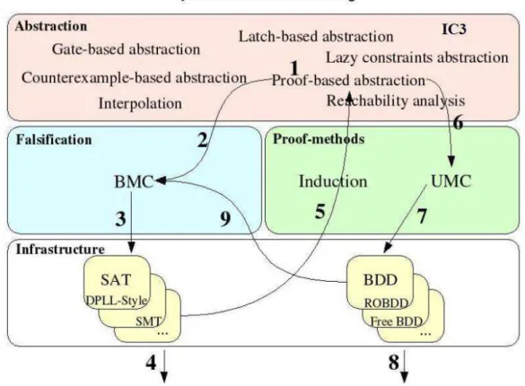
2.3. Symbolic Model Checking 31
Figure 2.8. Graphical visualization of Proof-based abstraction algorithm.
2.3.3.6 Reachability constraints
Given a finite state machine (FSM) of a hardware design, a statetis said to be reachable from s if there is a sequence of transitions that start from s and ends at t.
BDD-based symbolic traversal techniques to perform a reachability analysis on the abstract model can be used to compute an over-approximate reachable set for the concrete design. These are used as additional reachability constraints during proofs by induction or SAT-based Unbounded Model Checking.
2.3.3.7 Interpolation
An interpolant I for an unsatisfiable formula A∧B is a formula such that:
1. A→I
2. I∧B is unsatisfiable and
32 Chapter 2. Formal Verification
Intuitively, I is the set of facts that the SAT solver considers relevant in proving the unsatisfiability ofA∧B.
The interpolation-based algorithm [59] uses interpolants to derive an over-approximation of the reachable states with respect to the property. The BMC problem
BM C(M, p, k)is solved for an initial depthk. If the problem is satisfiable, a counterex-ample is returned, and the algorithm terminates. IfBM C(M, p, k)is unsatisfiable, the formula representing the problem is partitioned into P ref(M, p, k)∧Suf f(M, p, k), where P ref(M, p, k) is the conjunction of the initial condition and the first transi-tion, and Suf f(M, p, k) is the conjunction of the rest of the transitions and the final condition. The interpolant I of P ref(M, p, k) and Suf f(M, p, k) is computed. Since
P ref(M, p, k) → I, it follows that I is true in all states reachable from I(s0) in one step. This means that I is an over-approximation of the set of states reachable from
I(s0) in one step. Also, since I ∧Suf f(M, p, k) is unsatisfiable, it also follows that no state satisfying I can reach an error in k −1 steps. If I contains no new states, that is, I →I(s0), then a fixed point of the reachable set of states has been reached, thus the property holds. I I has new states thenR’ represents an over-approximation of the states reached so far. The algorithm then uses R’ to replace the initial set I, and iterates the process of solving the BMC problem at depth k and generating the interpolant as the over-approximation of the set of states reachable in the next step. The property is determined to be true when the BMC problem with R’ as the initial condition is unsatisfiable, and its interpolant leads to a fixed point of reachable states. However, if the BMC problem is satisfiable, the counterexample may be spurious since
R’ is an over-approximation of the reachable set of states. In this case, the value of
k is increased, and the procedure is continued. The algorithm will eventually termi-nate when k becomes larger than the diameter of the model. Figure 2.9 illustrates interpolation.
Procedure interpolation (M, p) 1. initialize k
2. while true do
3. if BMC(M, p, k) is SAT 4. then return counterexample 5. R = I
6. while true do
7. M’ = (S,R,T,L); let C = Pref(M’,p,k) and Suff(M’,p,k)
8. if C is SAT
2.3. Symbolic Model Checking 33
10. compute interpolant I of C;
R’ = I is an over-approximation of states reachable from R in one step
11. if R => R’ then return verified R = R or R’
12. end while 13. increase k 14. end while end
Figure 2.9. Graphical visualization of interpolation algorithm.
2.3.4
Proof engines
34 Chapter 2. Formal Verification
Since users have limited resources for the verification of systems, it is important to know which, of the huge number of available engines, are most effective. Imagine we take 5 different abstraction algorithms, together with 26 SAT solvers (26 is the number of SAT solvers competitors registered in the SAT Competition 2011 - http :
//www.cril.univ−artois.f r/SAT11/) and 1 BDD solver. The number of engines we get is 135 (5∗(26 + 1)). This shows that human intuition of the best engines to run becomes not so straightforward and selecting the best engines in an intelligent manner becomes a differential.
Chapter 3
Statistical Learning
Statistical learning plays a key role in many areas of science, finance and industry. Here are some examples of learning problems [47]:
• Predict whether a patient, hospitalized due to a heart attack, will have a second heart attack. The prediction is to be based on demographic, diet and clinical measurements for that patient.
• Predict the price of a stock in 6 months from now, on the basis of company performance measures and economic data.
• Identify the numbers in a handwritten ZIP code, from a digitized image.
• Estimate the amount of glucose in the blood of a diabetic person, from the infrared absorption spectrum of that person’s blood.
• Identify the risk factors for prostrate cancer, based on clinical and demographic variables.
The science of learning plays a key role in the fields of statistics, data mining and artificial intelligence, intersecting with areas of engineering and other disciplines.
In a typical scenario, we have an outcome measurement, usually quantitative (like a stock price) or categorical (like heart attack/no heart attack), that we wish to predict based on a set of features (like diet and clinical measurements). We have a training set of data, in which we observe the outcome and feature measurements for a set of objects (such as people). Using this data we build a prediction model, or learner, which will enable us to predict the outcome for new unseen objects. A good learner is one that accurately predicts such an outcome.
36 Chapter 3. Statistical Learning
The objective of supervised learning is to use the inputs to predict the values of the outputs. The inputs, that are measured or preset, constitute the set of variables. They have some influence on one or more outputs. In the statistical literature the inputs are often called the predictors, a term that will be used interchangeably with inputs, and more classically the independent variables. The outputs are called the responses, or classically the dependent variables.
The outputs vary in nature. They may be quantitative measurements or qualita-tive values from a finite set. For both types of outputs it makes sense to think of using the inputs to predict the output. This distinction in output type has led to a naming convention for the prediction tasks: regression, when we predict quantitative outputs, and classification, when we predict qualitative outputs. These two tasks have a lot in common, and in particular both can be viewed as a task in function approximation.
3.1
Multivariate regression
When fitting function for experimental data modeling have more then one independent argument we can talk about multivariate regression.
Despite the recent progress in statistical learning, nonlinear function approxima-tion with high-dimensional input data remains a nontrivial problem.
An ideal algorithm for such tasks needs to:
• avoid potential numerical problems from redundancy in the input data,
• eliminate irrelevant input dimensions,
• keep the computational complexity of learning updates low while remaining data efficient,
• allow for on-line incremental learning, and
• achieve accurate function approximation and adequate generalization.
3.2. Linear regression 37
Principal component analysis (PCA) is an important methodology that should be used when multivariate regression is in use. Its main objective is to find patterns in the input data, allowing the reduction of the number of dimensions without much information loss [75].
More recently k-nearest neighbors method has also been applied in conjunction with linear regression in different fields like semiconductor manufacturing.
3.2
Linear regression
The linear model has been a mainstay of statistics for the past 30 years and remains one of our most important tools.
There are many different methods to fit the linear model to a set of training data, but by far the most popular is the method of linear least squares. Used directly, with an appropriate data set, linear least squares regression can be used to fit the data with any function of the form
f(~x;~b) = b0+b1x1+b2x2+... (3.1)
in which
1. each explanatory (independent) variable xi in the function is multiplied by an
unknown parameter,
2. there is at most one unknown parameter with no corresponding explanatory variable, and
3. all of the individual terms are summed to produce the final function value.
In statistical terms, any function that meets these criteria would be called a “linear function”. The term “linear” is used, even though the function may not be a straight line, because if the unknown parameters are considered to be variables and the explanatory variables are considered to be known coefficients corresponding to those “variables”, then the problem becomes a system (usually overdetermined) of linear equations that can be solved for the values of the unknown parameters. To differentiate the various meanings of the word “linear”, the linear models being discussed here are often said to be “linear in the parameters” or “statistically linear”.
38 Chapter 3. Statistical Learning
f(x;~b) =b0+b1x+b11x2 (3.2)
is linear in the statistical sense. A straight-line model in log(x)
f(x;~b) = b0+b1ln(x) (3.3)
or a polynomial in sin(x)
f(x;~b) =b0 +b1sin(x) +b2sin(2x) +b3sin(3x) (3.4)
are also linear in the statistical sense because they are linear in the parameters, though not with respect to the observed explanatory variable.
Just as models that are linear in the statistical sense do not have to be linear with respect to the explanatory variables, nonlinear models can be linear with respect to the explanatory variables, but not with respect to the parameters. For example,
f(x;β~) =β0+β0β1x (3.5)
is linear in x, but it cannot be written in the general form of a linear model presented above. This is because the slope of this line is expressed as the product of two parameters.
Linear least squares regression also gets its name from the way the estimates of the unknown parameters are computed. In the least squares method the unknown parameters are estimated by minimizing the sum of the squared deviations between the data and the model. The minimization process reduces the overdetermined system of equations formed by the data to a sensible system of P equations in P unknowns (whereP is the number of parameters in the functional part of the model). This new system of equations is then solved to obtain the parameter estimates.
Nonlinear least squares regression could be used to fit this model, but linear least squares cannot be used.
In our work, we have:
f(x;~b) =Y
i
xbi
i (3.6)
Then, it can be linearized via:
logf(x;~b) =X
i