U
niversidade de
S ˜
ao
P
aulo
I
nstituto de
F´
isica
Mecˆanica Estat´ıstica de Sistemas Econ ˆomicos
Jo˜ao Pedro Jeric ´o
Orientador: Renato Vicente
Tese de Doutorado apresentada ao Instituto de F´ısica para a obtenc¸˜ao do t´ıtulo de Doutor em Ciˆencias
Banca examinadora:
Prof. Dr. Renato Vicente (IME-USP)
Prof. Dr. Nestor Felipe Caticha Alfonso (IF-USP) Prof. Dr. Fernando Tadeu Caldeira Brandt (IF-USP) Prof. Dr. Andr´e Cavalcanti Rocha Martins (EACH-USP) Prof. Dr. Masayuki Oka Hase (EACH-USP)
FICHA CATALOGRÁFICA
Preparada pelo Serviço de Biblioteca e Informação
do Instituto de Física da Universidade de São Paulo
Andrade, João Pedro Jericó de
Mecânica estatística de sistemas econômicos. São Paulo, 2016.
Dissertação (Mestrado) – Universidade de São Paulo. Instituto de
Física. Depto. de Física Geral.
Orientador: Prof. Dr. Renato Vicente
Área de Concentração: Física Estatística.
Unitermos: 1. Mecânica estatística; 2. Economia; 3. Inferência
Bayesiana; 4. Processos estocásticos.
A C K N O W L E D G E M E N T S
I offer my deepest thanks to my advisor, professor Renato Vicente, for his dedication and patience throughout this PhD, for the great deal of advices and for playing a large role in my personal and professional development.
I am also very thankful to Nestor Caticha for introducing me to Statistical Mechanics with his usual excitement ten years ago and showing a motivating interest to any problems or questions I presented him with.
I thank Matteo Marsili for receiving me for an internship at the ICTP in Trieste and for the fruitful collaboration we had. Also, thanks to the friends I made in Italy: Valerio, Ryan, Daniele, Matteo, Asja, Federico, Antonio, Erica and others without whom living in another continent would have been a much daunting task. Also Bruno being there helped a lot with this too, so thanks! I am also grateful to the Abdus Salam ICTP for the hospitality in hosting me.
I specially thank Andr´e and Paulo for sharing with me the highs and lows of doing a PhD during these four years. It was tremendously important and it would have been much harder without them. The same goes for Bruno, Gabriel, Lucas, Henrique and Petre, whom I have known for ten years now and whose friendship I treasure highly, even when some of them call me at5am fully aware that there is a4hour time difference between us.
I thank the people at the Statistical Physics group in IFUSP: Andr´e, Diogo, Carol, Cinthia, Jonatas, Rafael and others, for the interesting discussions, weekly seminars and friendly conversations. I also thank the people at work: Caio, Danilo, Darlan, Djalma, Luciano, Luiz, Marcelo and Paulo for their support during this last year dur-ing which I wrote this thesis. I specially thank them for the daily nag of when this thing would be done already.
I am grateful to CNPq and FAPESP for the financial support of my PhD, the latter under grant n. 2012/19521-8and also under grant n. 2014/16045-6for the internship abroad via the BEPE program. I also am very grateful to Dropbox for keeping all my PhD work nice and tidy in their servers. Seriously though, super helpful.
I want to thank both my families, Jeric ´os, Andrades, Vasarinis, Quinis and Lopes, for giving me the sense of belonging and security nothing else can. Special thanks to my parents, M´arcia and Jo˜ao Pedro, whom I will be forever indebted to for their unwavering support over all these years, giving me a safety net that allowed me to pursue my education with no restraints.
Finally, I would like most of all to thank Marina, for the life we are building together.
R E S U M O
Nesta tese, exploramos o potencial de ser usar t´ecnicas de Mecˆanica Estat´ıstica para o estudo de sistemas econ ˆomicos, mostrando como tal abordagem pode contribuir significativamente ao permitir o estudo de sistemas complexos que exibem compor-tamentos ricos como transic¸ ˜oes de fase, criticalidade e fases v´ıtreas, n˜ao encontradas normalmente em modelos econ ˆomicos tradicionais. Exemplificamos este potencial atrav´es de trˆes problemas espec´ıficos: (i)um framework de Mecˆanica Estat´ıstica para lidar com consumidores irracionais, no qual a racionalidade ´e controlada pela tem-peratura do sistema, que define o tamanho dos desvios do estado de m´axima utili-dade. Mostramos que um consumidor irracional aumenta a atividade econ ˆomica ao mesmo tempo que diminui seu pr ´oprio bem estar; (ii) uma an´aise usando Teoria da Informac¸˜ao de matrizes Input-Output de economias reais, mostrando que os m´etodos de agregac¸˜ao utilizados para constru´ı-las provavelmente subestima a dependˆencia das cadeias de produc¸˜ao em certos setores cruciais, com consequˆencias importantes para a anal´ıse destes dados; (iii)um modelo em que agentes com uma riqueza inicial dis-tributida como lei de potˆencias trocam aleatoriamente objetos com prec¸os distintos. Mostramos que esta desigualdade inicial gera uma desigualdade ainda maior em din-heiro livre, reduzindo a liquidez total na economia e diminuindo a quantidade de trocas. Discutimos as consequˆencias dos resultados destes trˆes problemas, bem como sua relevˆancia na perspectiva geral em Economia.
A B S T R A C T
In this thesis, we explore the potential of employing Statistical Mechanics techniques to study economic systems, showing how such an approach could greatly contribute by allowing the study of very complex systems, exhibiting rich behavior such as phase transitions, criticality and glassy phases, which are not found in the usual economic models. We exemplify this potential via three specific problems: (i) a Statistical Me-chanics framework for dealing with irrational consumers, in which the rationality is set by a parameter akin to a temperature which controls deviations from the maximum of his utility function. We show that an irrational consumer increases the economic activity while decreasing his own utility; (ii) an analysis using Information Theory of real world Input-Output matrices, showing that the aggregation methods used to build them most likely underestimated the dependency of the production chain on a few crucial sectors, having important consequences for the analysis of these data;(iii)
a zero intelligence model in which agents with a power law distributed initial wealth randomly trade goods of different prices. We show that this initial inequality gener-ates a higher inequality in free cash, reducing the overall liquidity in the economy and slowing down the number of trades. We discuss the insights obtained with these three problems, along with their relevance for the larger picture in Economics.
C O N T E N T S
1 introduction 11
1.1 Results of this thesis 12 1.2 Organization of this thesis 16
2 economics and the general equilibrium theory 19 2.1 A Brief Exposition 19
2.2 Limitations of General Equilibrium 24 3 statistical mechanics and inference 27
3.1 Statistical Mechanics as an inference problem 27 3.2 In Economics 33
3.3 The Role of Dynamics 36
4 the random linear economy model 39
4.1 The Model Ingredients 39
4.2 The Role of Statistical Mechanics 43 4.3 Regime change at n=2 46
5 inefficient consumer in a general equilibrium setting 51 5.1 The Irrational Consumer 52
5.2 Unobserved Utility 55 5.3 Conclusion 57
6 input-output of random economies and real world data 59 6.1 Input-Output Economics: Definitions and stylised facts 60
6.2 Loss of information via aggregation 65 6.3 Conclusion 71
7 when does inequality freeze an economy? 73 7.1 The model 75
7.2 The case of one type of good 77 7.3 The case ofKtypes of goods 83 7.4 Conclusions 89
8 conclusion 93
a calculation of the partition function for the random linear
economy model 95
b definitions 105
b.1 Spearman Rank Correlation 105 b.2 Kolmogorov-Smirnov distance 106 b.3 Bayesian Information Criterion (BIC) 107
1
I N T R O D U C T I O NThe wide perspective opening up, if we think of applying this science to the statistics of living beings, human society, sociology and so on, instead of only to mechanical bodies, can here only be hinted at in a few words. [14]
Describing the behavior of a large system composed of a large number of small parts for which we know the rules of individual behavior is the main theme of sta-tistical mechanics. It is successful in this regard because at large system sizes the variation in individual behavior, for which we despite knowing the rules we can not measure precisely, is irrelevant: the aggregate quantities are robust and predictable. However, there is no reason to believe this applications are limited to the traditional physics jurisdiction of gases, condensed matter, etc. Any system large enough that its uncertainties can be aggregated into robust properties can be studied using the tools of statistical mechanics: proteins composed of hundreds of aminoacids have a very large number of ways to fold themselves in three dimension, but the rules of attrac-tion for individual aminoacids makes it possible to calculate the probability of certain folding configurations [22]; The opinion of an individual is impossible to predict and model precisely, but the voting patterns or the opinion on moral issues of a nation comprised of millions of unpredictable individuals can be modelled with good accu-racy [42,89]; An aggregation of neurons with local firing rules can generate a neural network capable of storing and remembering patterns [46].
This large range of applications was made more explicit when E.T. Jaynes showed that the methods of statistical physics can be derived not only as a consequence of thermodynamics and physical laws but as the solution of an inference problem fol-lowing Shannon’s Information Theory [49]. A century later Boltzmann’s prescience turned out to be accurate.
In Economics, traditional theory usually describes the behavior of economic actors such as consumers and firms as the result of rigorous mathematical deduction from a few starting axioms of behavior. From there, one typically deduces the properties of an economy by treating this behavior as the average representative of a larger set of actors. However, this is only valid when interactions among actors is very negligible. When economic actors interact, as they often do, the possibilities are much richer
than the representative agent approach allows [18]. A Statistical Mechanics approach could greatly contribute to the field of Economics since it allows for the study of very complex systems, exhibiting rich behavior such as phase transitions, criticality and glassy phases, which are not found in the usual economic models.
The aim of this thesis is to make the case that the intersection of these two fields has a very large potential, being essentially two domains of knowledge that study very similar problems with different dressings: the properties and characteristics of interacting systems.
1.1 results of this thesis
The second part of the thesis concerns the three problems worked during this PhD:(i)
an approach for consumers that do not strictly maximize their utility in the Random Linear Economy model, (ii) comparison of the Input-Output tables for real world countries and the ones obtained in the random economies and (iii) the impact of inequality when randomly trading goods of different prices. We now briefly describe each of them.
1.1.1 Inefficient consumer in a general equilibrium setting
In Chapter5we extend the Random Linear Economy model introduced in Chapter4 by considering the cases where the consumer does not strictly maximizes his utility when choosing a bundle of M goods x = (x1, . . . ,xM), starting from his endowment x0 = (x10, . . . ,x0M), in a market composed of N firms each with a random technology
xi = (xi1, . . . ,xiM) and scalar scale of production si 0. In the original model, the consumer’s choice x is given by the Gibbs distribution at the zero temperature limit, that is,
x⇤ =arg max x
lim
b!∞
1
Ze
bU(x)d(x x
0
N
∑
i=1
sixi) (1) We make the case that the best way to model a suboptimal utility choice is by re-moving the zero temperature limit, or b ! ∞, and adjust how much the consumer
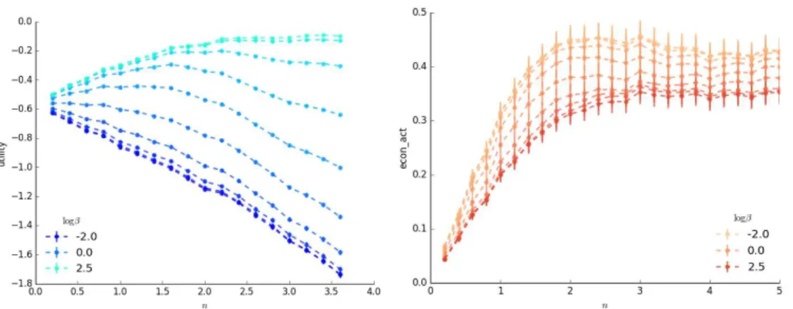
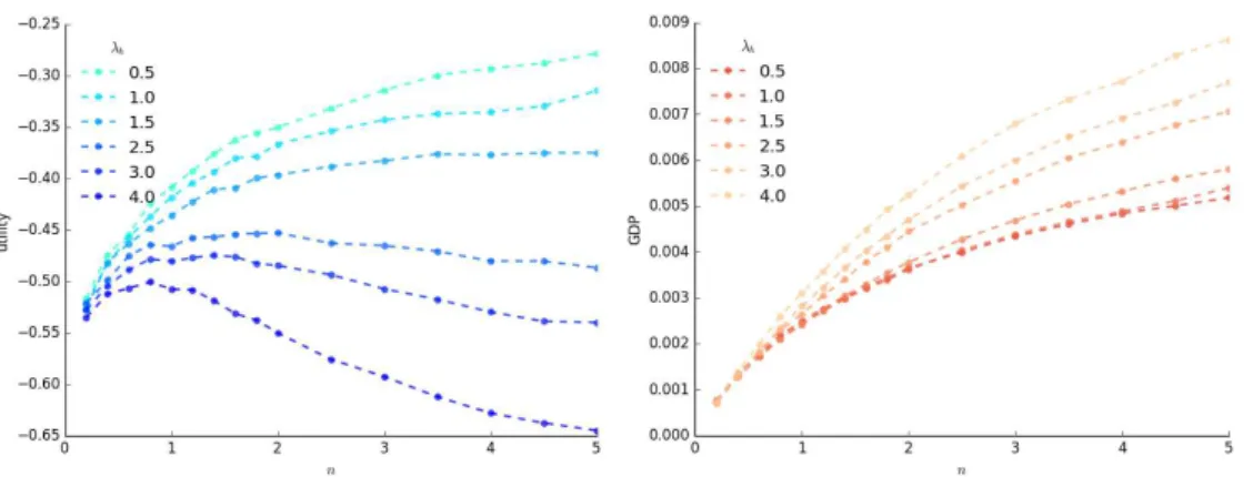
deviates from ”rational” behavior by changing b. By lifting this simple restriction we obtain nontrivial behavior, as shown on Figure 1. On the left, we show the agents utility as a function of the number of technologies per good n = N/M for different values of logb. When bis large (around 102), the agent optimizes efficiently enough that his utility always increases with n. However, when b gets lower and the repre-sentative consumer starts making worse choices (according to his utility function), his expected utility in the marketdecreaseswithn instead of increasing.
1.1 results of this thesis 13
Figure1.:(Left) Average consumer utility per good as a function of the number of technologies per goodn, for several degrees of inefficiency b(whenb! ∞, the consumer strictly maximizes his utility). A largen means there are more trades available for the consumer and a rational consumer should always increase his utility when faced with a growing number of possibilities. This is not the case for a consumer that chooses inefficiently.(Right)Average economic activity (volume of goods exchanged per good) as a function ofn, for several degrees of inefficiency. An inefficient agent may choose poorly when faced with many choices, but he trades a larger quantity of goods.
of his choices [47, 76]. What is more interesting is that the economic activity in the market, in this case measured by the density of goods being exchanged,increaseswith the inefficiency in consumer choice, because he deviates a lot more from x0 than if
he were strictly maximizing his utility. In this stylized economy, markets with agents that make bad decisions have unhappier agents but are more active and, considering economy activity is usually correlated with wealth, richer.
This work has been submitted as Jeric ´o, J.P., Vicente, R. (2016)Information inefficiency in a random linear economy model. Europhysics Letters
1.1.2 Input-Output of random economies and real world data
In Chapter 6 we collect several years of the Input-Output tables for ten real world economies, which are matrices showing how much the industries of each sector of the economy produce and use as input of every good in the economy. The goods are also divided in the same sectors as the industries, in the case of the US at three levels of aggregation: detailed level, with 389 sectors, aggregated with 71 and summary with 15, going from ”Mining” in the summary level to ”Coal mining”, ”Iron, gold, silver mining”, etc, in the detailed level, and at two levels of aggregation for the EU countries: 64and10levels.
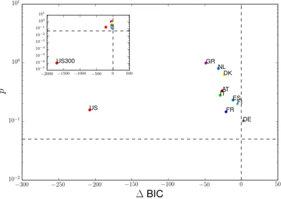
goods as nodes, and by definition the indegrees (sum of all edges that point to the node) are equal to one. The outdegrees, however, are variable, and they indicate the dependency of the production network on a specific good. Acemoglu et al [2] show that the heavier tailed the outdegree distribution is, the more susceptible to shocks is an economy.
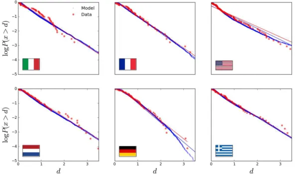
Figure2.: Log of the counter cumulative degree distribution for six of the ten countries analyzed, com-pared with the closest degree distribution generated by the Random Linear Economy model with M= 100, b ! ∞ for different values ofn. Both datasets are plotted along with their regression, which is very close to an exponential distribution.
We show that the outdegree (or simply degree) distribution of ten countries we have analysed at the aggregated level (64sectors for the EU,71 for the US) is very close to an exponential distribution, whereas data at the detailed level of aggregation for the US has much heavier tails. Given that these degrees are random variables with a fixed average, Information Theory tells us that in the absence of any extra constraints the distribution that maximizes entropy is an exponential distribution. This allows us to conjecture that the aggregation process has washed out the structural information of the economy.
1.1 results of this thesis 15
a direct consequence on Acemoglu et al’s conclusion for the structural fragility of the US economy: distribution tails that were taken into account may have been a simple artifact of the aggregation process, and the real distribution may be heavier tailed than what they calculated. If this is the case, the predictions made on [2] concerning the fragility of the U.S. economy to random shocks may have been underestimated.
This work was accepted for publication as Jeric ´o, J.P., Marsili, M. (2016)Input Output of random economies and real world data. Eur. Phys. J. Special Topics: Can economics be a physical science?
1.1.3 When does inequality freeze an economy?
In Chapter7 we show the statistical effects of inequality in a simple trading economy where we have N agents with a initial capital that is power law distributed P(ci > c)⇠c b, and agents tradeM goods each with its own pricep1, . . . ,pM, such that the leftover cash of an agent is its capitalciminus the price of the goods he owns. At each trading step, one of the M goods is chosen at random and its owner tries to sell it to another agent, which automatically accepts it if he has enough cash to do so.
The parameters are set in such a way that even the most expensive good is affordable to the poorest agent. Despite that, in the stationary state we show that this zero intelligence dynamic divides the agents into ”classes” where an agent can afford goods up to a certain price and none more expensive than this threshold. If we define an agent’s leftover cash as his liquidity in the market, given a unequal distribution of capital the economy’s liquidity concentrates into fewer agents, and as the inequality parameter b goes to one, the economy freezes completely as only the richest agents carry any meaningful trade.
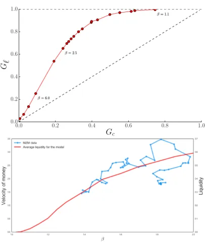
These results are summed up by the top panel of Figure3. There we plot the Gini coefficient for the cash as a function of the Gini coefficient for the capital. The Gini coefficient is a measure of inequality in a distribution and goes from zero to one: zero means perfect equality, all data in the dataset are the same. One means perfect inequality: only one point is positive and the rest is all zero. In Figure 3, we show that liquidity in the model is always much more concentrated than the initial capital, converging to perfect inequality when b ! 1. This has an arresting effect where all trade in the economy stops. This result is tested versus empirical data in the bottom panel of Figure 3, where we compare the velocity of money, as defined by the US Federal Reserver Bank, as a function of the inequality for the model and the historical US data, showing that there is good corroboration that inequality indeed decreases the velocity of money.
Figure3.:(Top) Gini coefficient G` of the cash distribution (liquid capital) in the stationary state as
a function of the Gini Gc of the capital distribution, for numerical simulations described in
Chapter7. Cash, or liquidity, is always more unequally distributed than capital, resulting in perfect inequality (when only a countable number of agents have non zero liquidity) whenb approaches one. (Bottom)Velocity of money, defined for the model by equation (119), as a function of the level of inequality represented by the power law parameterb, with comparison to the historical US data. Our model corroborates the fact that as inequality increases, the number of money units that are exchanged in a time interval decreases.
1.2 organization of this thesis
1.2 organization of this thesis 17
In Chapter 3, we will make the case of why Statistical Mechanics is a suitable tool for exploring and studying Economics. Although the Physics minded reader most likely does not need much convincing, it is still useful for those that never had any exposition to a general, information theoretical approach to Statistical Mechanics as introduced by Jaynes [49]. We hope that a reader with a background in Economics (and who hopefully did not stop reading the thesis after Chapter 2) will agree with us that the methods presented therein offer an alternative to the usual methods in Economics. In this chapter we will also present a number of previous work that have already explored this intersection.
We end the first part by introducing the Random Linear Economy model in Chapter 4, which consists of a simple market model where companies have random technolo-gies and one consumer wishes to improve his utility by trading his current goods in the market, which is exactly the sort of problem General Equilibrium Theory describes. Despite its simplicity, the model exhibits a rich behavior due to the stochasticity intro-duced in the technologies and its solution is arrived at by using techniques from the Physics of disordered systems. Its introduction merits a dedicated chapter because not only it serves as the basis for the work developed on Chapter5and parts of Chapter 6, but also because it is a good representative of the ideas put forward in Chapters 2 and3.
2
E C O N O M I C S A N D T H E G E N E R A L E Q U I L I B R I U M T H E O R YIn this chapter we will give a background of the relevant economic theory for this thesis. We aim to formally introduce a central theory in economics which is General Equilibrium Theory. Along with it, we hope to expose the reader with Physics back-ground to the usual concerns of Economics. We also discuss the common criticisms about General Equilibrium Theory, along with more recent work to solve some of the problems discussed.
General Equilibrium Theory is a mature field of Economics [9, 57, 58] which aims to characterize the existence and properties of equilibria in certain market settings. Economic systems are frequently assumed to have actors with opposing goals: the owner of a good wants to sell it for the highest possible price, while its potential buyers would like to purchase it for as low as possible. Fishermen would like to catch as many fishes as possible and expect their peers to not also overdo it otherwise they may extinguish the oceans. Businessmen would like to price their products in such a way that as many people as possible buy it for as high as possible. A couple in vacation would like to buy a plane ticket to Paris as cheap as possible as long as the layover is not longer than a couple of hours. One expects that economies and markets composed of many such actors trying to get their way will converge to a certain steady state. The main goal of General Equilibrium Theory is trying to characterize these equilibrium states in a rigorous manner. In this sense, it’s a microeconomic theory, because it explains macrobehavior from the incentives (or micromotives [78]) of agents.
While the work in this thesis doesn’t strictly aim at studying economies as they are described in General Equilibrium Theory, its purposes and questions are very similar to the ones physicists usually ask when studying a complex system: namely, the characterization of its equilibrium state. It’s important, therefore, to have a deeper understanding of how this is done in economics, what are its main concerns and assumptions, if only to realize the two field have very similar goals.
2.1 a brief exposition
The exposition in this chapter is mostly adapted and simplified from Mas Colell’s seminal book on Microeconomic Theory [57] and will be considerably more formal than the rest of this thesis due to the way the discipline is commonly studied.
In General Equilibrium Theory, an economy is defined through the following com-ponents: we assume there are J consumers, N firms and M goods in a market. Each consumer has a consumption set Xj which contains all possible consumption bundles xj = (x1j, . . .xjM) that the consumer has access to, i.e., each bundle xj is a M dimensional vector with nonnegative entries (we are assuming he cannot con-sume a negative amount of a good). Xj is limited by “physical” constraints, such as no access to water, iron or bread, but not monetary constraints, which we will deal with later.
The consumer also has an utility function Uj(x) that takes every element xj 2 Xj to a real number, representing how much the consumer values each bundle of his consumption set. This allows us to define define a preference relationship over the elements in Xj (i.e., if the consumer prefers bundle x to x0), which is complete1 and transitive2, two standard requirements in Economics for rational behavior.
Finally, the consumer is also endowed with an initial bundle of goodswj = (w1j, . . . ,wjM),
wµj 0 which will define his budget given a set of prices for the goods and will con-straint his choices on Xj. His initial budget is defined in terms of a bundle of goods for two reasons: first, we want the economy as a whole to be unaffected by the scales of prices, so if all prices are multiplied by a constant factor the consumer’s purchasing power remains the same. Second, the theory described general equilibriums, which are assumed to be valid for closed markets. All goods used as input have to come from somewhere inside the economy, and the consumer acts as the provider of raw material.
Each firm ihas a production set Ξi of technologiesxi = (x1i, . . . ,xiM)that it is able to operate. Unlike consumption bundles, which are final allocations and therefore must be nonnegative, technologies can be any real number: the negative entries are inputs and the positive entries are outputs in the technology’s operation. Ξi is also
limited only by “physical” constraints, not by monetary constraints. A firm that has
xi = ( 1, 2) in its production set is able to transform one unit of good 1 into two units of good 2. It won’t necessarily be able to transform two units of good 1 into four units of good2, for that it must also havex0i = ( 2, 4)inΞi. It might be the case,
for example, that companies get more efficient with production and therefore it might havex00i = ( 2, 6)in its production set.
In General Equilibrium Theory, an economy is formally defined as the tuple
E=⇣{(Xj,Uj)}Jj=1,{Ξi}
N
i=1,{wj}Jj=1
⌘
. (2)
One of the theory’s assumptions is that the economy described is complete, which means every agent can exchange every good with no transaction costs and complete information about the firm’s technologies, other consumer’s consumption, etc. Also, a
1 For everyx,x02Xj, eitherUj(x) Uj(x0)orUj(x)Uj(x0).
2.1 a brief exposition 21
goodµcontains all the possible information that a consumer would take into account when making his choice. That is, among the space of goods we could have “umbrella” and “chocolate”, or we could also have “an umbrella on August 13th, 2016 in S˜ao Paulo with50% chance of rain” and “an umbrella on December12th,2016in Chicago with90% chance of rain”. There is no hidden information, so the consumer is never in doubt of whether the good or company is actually reliable or any such considerations.
It’s also assumed that agents areprice-takers, that is, they are unable to affect the market prices and therefore have to take them as a given. The prices of the goods are given by a M dimensional vector p = (p1, . . . ,pM), where each price is a strictly positive quantity, i.e., pµ > 0 for all µ. This carries the restriction that goods have global prices, which is consistent with the completeness assumption: there is no rea-son why the market prices should be different for certain consumers or firms if they have complete knowledge and no transaction costs.
With a price vector pdefined, we say the consumerjhas a budgetBj = p·wj, which is the monetary value of his initial endowment. Any bundle he chooses to purchase will cost him p·xj. His objective, therefore, is to find the best bundle xj he is able to afford, that is:
max xj2Xj
U(xj), s.t. p·xj p·wj (3)
The firms, on the other hand, have an operating profit for each technology given by
p·xi, which is how much money they earn by selling their outputs (xµi > 0) minus how much they spend purchasing the inputs (xµi <0). Their objective is to maximize
their profits, that is:
max
xi2Ξi
p·xi (4)
With these ingredients laid out, we define anallocationof the economy as a set of specific choices for consumption bundles and technologies, i.e., an allocation a of an economyEis
a = (x1, . . . ,xJ,x1, . . . ,xN), xj 2 Xj, xi 2 Ξi (5) We are considering closed economies and therefore all that is produced must come from the initial endowments and end up part of the consumers’ final bundles. We therefore say an allocation isfeasibleif it satisfiesmarket clearingfor all the goods:
J
∑
j=1
xµ j =
J
∑
j=1
wµ j +
N
∑
i=1
xµ
This is a strong condition which couples many quantities in the economy. In partic-ular, if we multiply both sides of the equation by pµ and sum overµwe get, in vector notation,
J
∑
j=1
p·(xj wj) = N
∑
i=1
p·xi (7)
The left-handside is the leftover money the consumers have after making their choice of consumption, also called the value of excess demand, whereas the right-handside is the firms aggregate profit, also known as the value of excess supply. Be-cause we assume that the consumer may not spend more than his budget, the value of each consumer’s individual excess demand has to be non positive. Simultaneously, if we assume that firms always have xi = 0 in their production set, i.e., we assume that they can always opt to not produce at all and leave the market, then the value of excess supply for each firm has to be non negative. Because they must be equal, we conclude that in an economy for which market clearing holds, the consumer spends all his available budget and firms all get zero profit, a result known asWalras’ Law.
Given a set of feasible allocations{ak}, we may wonder if there is any allocation we desire most over the others. This of course depends on the criteria we use to judge them: we may like allocations with less inequality, with the most aggregate utility, with the smallest minimum utility, etc. Economists opt to use one particular condition which is calledPareto optmality.
Intuitively, a Pareto optimal (or Pareto efficient) allocation is one in which you can’t make a consumer better without making another consumer worse off. The idea is that, a non Pareto optimal allocation has some waste in it: one could change the consumption bundles in order to increase some utilities and no other consumer would complain. Because firms have zero profit in feasible allocations, they wouldn’t mind the change.
More formally, a feasible allocation a = (x,x) is said to be Pareto optimalif there is no other allocation that Pareto dominatesit, that is, no allocationa0 = (x0,x0)such
thatU(x0j) U(xj)for all jandU(x0j)>U(xj)for at least one j.
The Pareto optimality concept therefore defines a socially desirable outcome in a “non-controversial” way, by definition no agent in the economy would have a problem with policies or actions taken to make it more Pareto efficient. However, it says nothing about equality: an allocation in which one consumer has all the goods and no other consumer has any goods is Pareto optimal.
We finally arrive at the concept of equilibrium in an economy. A Walrasian equi-librium (or competitive equilibrium or simply equilibrium) in an economy E is an allocation(x⇤,x⇤)and a price vector psuch that
1. Every firmimaximizes its profits in its production setΞi, that is
2.1 a brief exposition 23
2. Every consumerjmaximizes his utility in his consumption setXj, that is U(x⇤j) U(xj), 8xj 2Xj, 8j2 {1, . . . ,J} (9)
3. The allocation(x⇤,x⇤)is feasible, that is,
J
∑
i=j x⇤j =
J
∑
j=1
wj+ N
∑
i=1
xi⇤ (10)
The Walrasian equilibrium is essentially a pair allocation - prices such that all opti-mization problems are solved at once. Although we have not mentioned any dynamics in this economy, it’s considered an equilibrium because all agents are as satisfied as possible with their allocation given the prices, which we have assumed to be global and unchangeable by any agent’s action. This is not exactly a definition of equilibrium as used in Physics, but we will discuss this point later. For now, we point out that a Walrasian equilibrium is in some sense stable.
We have thus defined two desirable properties of an allocation: efficiency and equi-librium. The fundamental results of General Equilibrium Theory are the Welfare Theorems, which define the conditions for which an equilibrium is Pareto optimal and for when a specific Pareto optimal allocation is an Walrasian equilibrium.
The First Fundamental Welfare Theoremasserts that if the consumers have a con-tinuous utility function on Xj3, then all Walrasian equilibria are Pareto optimal. This result is simple yet useful, because it tells us that if our economy is in equilibrium, we don’t have to care about checking if it’s efficient. The violation is also important: if a given economy we are studying is in an inefficient equilibrium, then it must be that one of the theorem’s condition was violated. This sheds light in where to look for mar-ket failures. We remind the reader, however, that some extra strong assumptions were made for the economies described by this theorem, namely, completeness of market and global prices that no single agent is capable of influencing.
The Second Fundamental Welfare Theoremrequires extra assumptions: it affirms that if an economy satisfies the conditions of the first fundamental theorem, the utility functionsUj and all setsXj,Yi are convex and if we are able to redistribute the initial endowments at will, while keeping the total amount∑jJ=1wj constant, then for every Pareto efficient allocation there exists a wealth allocation w and price vector p⇤ such that(x⇤,x⇤,p⇤)is a Walrasian equilibrium.
The second theorem is considerably more interesting than the first one: any Pareto optimal allocation we would like in an economy can be an equilibrium given the ap-propriate price vector and a possible wealth transfer, albeit under a stronger set of conditions. It serves both as a benchmark, because we know what we can expect from
markets at their ”optimal conditions”, but also as a warning: we can only guarantee that an efficient allocation will be an equilibrium under a very strong set of require-ments.
2.2 limitations of general equilibrium
A conspicuous element was missing from the exposition above: there are no rules for the dynamics of the economies described above. The prices are taken as a given, as are the consumer and firm choices. What happens if a firm closes? What happens if a new firm appears? The equilibrium is simply “recalculated” and the economy moves to the new one?
Indeed, this is a long standing criticism to General Equilibrium Theory. Walras proposed it as a process of tat ˆonnement4: a central figure, known as the Walrasian auctioneer, suggests a price and asks all the firms and consumers how much would they like to produce and buy at these given prices, but without any transaction taking place at out of equilibrium prices. The auctioneer updates the prices in the direction of diminishing excess demand or supply, a gradient descent process, until equilibrium is reached, at which point transactions finally take place. The auctioneer must also have a way of guaranteeing that agents will be price takers: it must either be able to monitor and enforce all transactions or buy and sell arbitrary amounts of every good at their equilibrium prices.
It is clear that such process is very convoluted. Chiefly, this auctioneer figure doesn’t exist in most decentralized markets: goods are traded at agreed prices by both parts, which do not wait until their transaction is authorized by some central authority. Even if there were auctioneers, such authority would require an infinitely large computa-tional capability to compute the excess demand and supply of every consumer and firm and for every good in a modern economy [11,69]. Worst of all, even if there was such central figure with such an arbitrary large amount of computing power, not all price updating dynamics are guaranteed to converge [44]. Finally, even if it converges, we have no assurance that it will converge in finite time.
These are all well known and acknowledged shortcomings of the theory. Some ar-eas of Economics, such as the Schumpeterian Economics [75], eschew the ideal of an static equilibrium altogether, studying the pattern of changes from certain evolution-ary rules instead. These ideas are also popular amongst physicists [86].
However, the usefulness of General Equilibrium Theory in Economics stands not from practical applications, but as a benchmarking tool for real world policies. Their conclusions are mathematically precise and correct. So when faced with an economic equilibrium that is not Pareto efficient, then by definition it must be because one of the Second Fundamental Welfare Theorem conditions was violated, and therefore one knows where to look for inefficiencies to try and fix it.
2.2 limitations of general equilibrium 25
Decades after the introduction of the Welfare Theorems, the field of Applied Gen-eral Equilibrium arose as a way to compute equilibria and explore them for policy decisions [79,80]. It used real world data to calibrate production and utility functions along with iterative schemes to calculate the equilibrium prices [72]. From there, it could be used to explore the impact of policy changes in more complex settings.
More recently, these limitations have been tackled by the Dynamic Stochastic Gen-eral Equilibrium (DSGE) models, that have origin in the work by Kydland and Prescott [55]. In that seminal paper, the authors calculate the evolution in time of macroeco-nomic variables such as ecomacroeco-nomic output over time by treating it as the trajectory in time of a microeconomic general equilibrium problem with stochastic elements. This has led to a new class of economic models based on this approach of using dynami-cal systems with stochastic terms and inferring the parameters from real world data [27,83], which are employed today by institutions such as the European Central Bank for policy analysis [82].
However, what all of theses models have in common is that they all look for equi-libria in the Classical Mechanics sense of Physics. Generally speaking, an equilibrium state in Economics is when all incentives cancel each other out and no actor has the desire or the possibility of deviating from the current configuration, which is an ap-proach that heavily draws from Classical Mechanics in Physics and dynamical systems in Mathematics. In fact, Stephen Smale even wrote a paper on the dynamics of Gen-eral Equilibrium [81] trying to tackle some of the open dynamical questions discussed earlier, employing modern mathematical theory of dynamical systems.
This Classical Mechanics approach has limitations: due to the need of having one ex-act solution for the equilibrium configuration, economic models usually employ some standard simplifications to make problems tractable. The most common of which is the representative agent, in which a single agent represents all consumers, another represents all firms, all the government policies, etc, and his objective functions are considered as the average of an heterogeneous population, with the different parts of the economy interacting through these ”average demands”.
agents allows for models in which crisis and transitions come from endogenous rules of interaction instead of arbitrary adhoc modelling.
But perhaps the biggest difference in the approaches is that, in Statistical Mechanics, an equilibrium is defined as an ensemble of possible configurations that appear with certain probabilities, and instead of trying to find the exact numbers that equilibrate the system, one looks for the average of macroscopic quantities. This allows for the interpretation of fluctuations as a natural phenomena, due to the nature of the uncer-tainty involved in inferring a complex system, as we will describe in the next chapter. Then, one can truly define the behavior of microscopic interactions, as opposed to representative agents, and say something about the aggregate.
3
S TAT I S T I C A L M E C H A N I C S A N D I N F E R E N C EIn this Chapter we aim at answering the question of why Statistical Mechanics is suitable to study economic systems. The essence of the answer is that, among other things, the techniques of Physics allows one to find the minimum energy configuration (or at least very good approximations) and the expectation value of certain quantities of interest in rather complicated settings, which is precisely what Economics could mostly benefit of.
To the reader familiar with Statistical Mechanics, we draw attention to the fact that we present here the canonical ensemble not as a derivation from Thermodynamics, but as a systematic inference of a system’s observables using Information Theory. Instead of assuming a system connected to a heat bath at a fixed temperature and employ-ing the first postulate of Statistical Physics, we follow the work of Jaynes [49] and show that the Gibbs distribution is the solution for an inference problem with limited information.
3.1 statistical mechanics as an inference problem
Suppose we have an interacting system composed of N particles, each with its own state xi, which can be its position, velocity, orientation, decision of whether to buy a Mac or a PC, political affiliation, etc. The whole system can be fully characterized by the configuration vector x = (x1, . . . ,xN) and we assume all the information we have about this system is the expected value of functionH(x), often called in physics settings the energy function. There are many questions we can ask about the system, for example what is the probability of this system being at a configurationx, or what is the expected value of another quantityG(x). These questions are inference problems, and through Information Theory we can find out what is the best way we can answer them.
As proposed by Shannon [77], when faced with a choice of several probability func-tions that describe some data or phenomena, one should always opt for that which
makes the least assumptions, given the constraints of the problem. This amounts to finding the probability distributionp(x)that maximizes theShannon entropy
S[p] = Z
dxP(x)logP(x) (11) subject to the constraints imposed by observation. In our case, the constraint is that the energy function H(x)has an average valuehH(x)i= R dx P(x)H(x) = Eand we also have to impose the constraint thatP(x)is a probability distribution and therefore must be normalized, i.e., R dx P(x) =1. This means that to find P(x)for our system, we must find P(x)that maximizes the Lagrangian
L[P] =
Z
dxP(x)logP(x) +a
✓Z
dx P(x) 1
◆
+b
✓Z
dx P(x)H(x) E
◆
, (12)
where aandbare the Lagrange multipliers of this maximization problem.
We assume that at the maximum P⇤ a small perturbation P(x) +dP(x) does not alter the Shannon entropy. If we assume that all dP(x) are independent (i.e., dP(x)
and dP(x0)are not correlated for every x,x0 in the support of the distribution), then
for everyx this becomes a regular maximization problem. For everyx, we must solve that dLd(PP)(x)is equal to zero, that is:
∂
∂P(x){ P(x)logP(x) +a(P(x) 1) b(P(x)H(x) E)}=0, 8x (13)
Solving this equation we have that for every value of x
logP(x) 1+a+bH(x) =0) (14) )P(x) =e 1+a bH(x) (15) The Lagrange multipliers must be set so that the constraints are satisfied. Forawe have thatea 1must normalize the probability distribution, i.e.
Z
dxe 1+a bH(x)=1) (16)
e1 a = Z
dxe bH(x) =Z (17) This normalization term is the sum over all the configurations and is called the
partition function. For bwe must have that
Z
dxH(x)e
bH(x)
Z =
∂
3.1 statistical mechanics as an inference problem 29
This means b must be such that the average energy of the system is equal to the observed averageE. However, suppose we have not actually observedE, all we know is that it is fixed to some value. Then, because E is given by the above equation for which the only degree of freedom is a Lagrange multiplier, all the possible values it can take are given by varyingbfrom0to∞. We have finally arrived at the maximum entropy distribution for our inference problem, which is theGibbs distribution
P(x|b) = 1 Z(b)e
bH(x) (19)
The extreme cases forbgive us an intuition on how the Gibbs distribution behaves. For b = 0, P(x) = 1
Z, for all values of x: in this limit all configurations are equally likely, regardless of their energyH(x). In the opposite case, whenb!∞, Zbecomes more and more concentrated around its maximum point, where E(x) is minimum, and eventually P(x) collapses to a delta function around the minimum energy con-figuration, also known as the ground state(it can also have an equal mass in several points in the case of multiple minima). Therefore, in the full b spectrum, the Gibbs distribution starts completely uniform in the space of all configurations and slowly co-alesces around the minimum energy values. If we assume H(x)is bounded, then for every finite value ofb, the system has a finite probability of being in any configuration (what is known as ergodicity). Given a system described by the Gibbs distribution, the average value of another desired observableG(x)is given by
g=hG(x)i= Z
dxG(X)1 Ze
bH(x) (20)
Though we have called H(x)the energy function for customary reasons, this func-tion is in principle any arbitrary funcfunc-tion of the system configurafunc-tion that has a well defined average value. For most systems of interest we can always decompose it as a sum of small scale interactions, that is, we can write
H(x) =
∑
aHa(xa), (21) where a represent minimal cliques, usually pairwise, where we can reduce the inter-actions in the system to microscopic interinter-actions. In this way, the behavior of macro-scopic quantities such as the average energy or any other observable we are interested depends on the sum of a large amount of simple interactions.
special interest because they represent some of the most interesting phenomena a sys-tem can present, and indeed, many popular questions in Economics, such as business cycles, crisis, altruistic cooperation, etc, can be framed in terms of phase transitions.
We note that despite this being the standard theory for the canonical ensemble in Statistical Physics, we have not made so far any Thermodynamical (or any other ”physical”) assumptions. We have been describing generic systems where we simply applied the tools of Information Theory for the inference of a random variable for which we have limited information. There’s nothing that limits us to using the Gibbs distribution only for gases in which the molecules interact according to the laws of Physics. This is the fundamental reason why Statistical Mechanics is so successful at explaining such a varied wealth of phenomena: despite being first developed via physical laws, its results are general.
The only real difference when dealing with a thermodynamical system is that when we plug the Gibbs equation back into the Shannon entropy we have
S[PG] =logZ+bE, (22) which is still general, but we can now use one of the Maxwell’s relations to give b a physical interpretation:
1
T =
∂S
∂E = b (23)
Therefore in physical systems b is identified as the inverse temperature and when
T ! ∞, the system is equally likely to assume any possible configuration. Likewise,
whenT=0, the system is frozen at one of the ground states.
3.1.1 A simple example
We make explicit the general nature of the Gibbs distribution deduced in this section by a simple example1 of a random variable x that can take three values: -1, 0 or 1. We know it’s average is hxi = m. What is the best inference we can make for it’s probability distributionP(x)? The Gibbs distribution is
P(x) = e
lx
Z(l), (24)
where Z(l)is given by:
Z(l) =
∑
x2{ 1,0,1}
e lx =1+2 coshl (25)
3.1 statistical mechanics as an inference problem 31
And lis given by
m= ∂
∂llogZ(l) =
2 sinhl
1+2 coshl (26)
Writing u = e l and writing the hyperbolic functions as 2 coshl = el+e l and
2 sinhl= el e l we have
u u 1
1+u+u 1 = m)m+ (m+1)u+ (m 1)u
1 =0 (27)
Multiplying both sides of the equation by u, we have the second order equation
(m 1)u2+mu+ (m+1) =0, for which the (positive) solution is
u= m
p
m2 4(m2 1)
2(m 1) (28)
Figure4.:(Left)EntropyH[P]for the Gibbs distribution of a random variablexthat takes three values, -1,0and1as a function of its known averagehxi=m.(Right)Probability distributionPG(x|m)
as a function ofmfor each of the three values.
And finally we find thatl= logu. We plot on Figure4the entropy for the Gibbs distribution as a function of m and the probability P(x|m) for the three values. We see that as expected entropy is maximal when the three states are equally likely, and whenm= ±1 the variable is fully identified, so the entropy goes to zero.
3.1.2 Optimization Problems
The Gibbs distribution offers a natural way of solving maximization problems: given a system that we know has energy function H(x), its ground state is simply the dis-tribution of states x at zero temperature, or at b ! ∞. Likewise, we can find any
This is certainly not the only way one can find solutions to optimization problems, however, framing it as a Statistical Physics problem has a couple of benefits, namely, if we accept approximate solutions, we can find them very close to the optimal in a time orders of magnitude smaller. Usually this is done using general purpose Monte Carlo algorithms to sample from the Gibbs distribution at a certainbvalue and slowly increasing bup (i.e., decreasing the system’s temperature) until convergence, a tech-nique known as simulated annealing. For well behaved convex functions there are certainly more efficient optimization algorithms, but Monte Carlo techniques are very robust and allow us to add constraints and interactions in the energy function without having to adopt an alternative maximization procedure.
As an example from [60], consider a conference planner that would like to distribute
N scientists in two available hotels. Scientists either like or dislike each other. We represent this by a positive interaction constant Jij = 1 if iand jlike each other and Jij = 1 ifiand jdon’t like each other. Scientists would then prefer to stay in hotels with their friends and not be in the same hotel with scientists they don’t like. If we represent the hotel that a scientist is bysi = ±1, the planner has to optimize for each scientistihis utility
ui(~s) = N
∑
j=1,j6=i
Jijsisj (29) And then his problem is to find the configuration~swhich maximizes the total utility
for all scientists, i.e.
U(~s) =
∑
i
ui(~s) =
∑
i,jJijsisj. (30) For as little as 3 scientists, the problem can be frustrated: if all Jij = 1 or if two are positive and one is negative, there are multiple ground states. For the general case, a brute force solution would require a search over 2N configurations, which is unfeasible even for conferences with N = 100 participants. However, with a Monte Carlo simulation we can find close approximations much more quickly.
This scenario, of course, is the Sherrington-Kirkpatrick model of a simplespin glass. Indeed, the theory of spin glasses are a very successful case in which complex systems with non regular patterns of interaction (also calleddisordered systems) can be stud-ied, often solved analytically and exhibit very rich and interesting behavior.
3.2 in economics 33
number of solutions to the number of available assets [43,41]. These aren’t suboptimal solutions due to high temperature, but optimal portfolios a perfectly rational agent would choose.
3.2 in economics
The utility of employing Statistical Mechanics to better model economic problems has not gone unnoticed by economists, even though it’s usage is far from mainstream. It is most frequently used in interaction based models, in areas such as Game Theory, which arose precisely to deal with situations in which the decision of one agent affects the payoff of another, and rising microeconomic fields such as Social Interactions [73].
Probably the most influential work to show how a large interacting population can lead to unexpected outcomes is Schelling work on segregation [74], where two types of agents live in a city and all agents prefer to live in neighborhoods where their type is slightly more common than the other. This search for optimality will lead to complete segregation of agents, despite everyone preferring to live in mixed areas. In Schelling’s words: ”there is no simple correspondence of individual incentive to collective results”. For a Statistical Mechanics treatment of Schelling’s segregation model, we refer the reader to [29].
One of the first major proposals of connecting Statistical Mechanics with Economics came from Santa Fe Institute’s seminal workThe economy as an evolving complex system
[4,10], which influenced physicists and economists alike.
Later, in [21] and [20], Brock and Durlauf describe an interacting model where each agentichooses between two binary actionswi = 1 orwi =1 and his utility function has three terms: a private, deterministic term u(wi), one that interacts with other agents via a Jwiwj utility interaction and a random shocke(wi)whose distribution is given by the probability thate(wi =1)is larger than e(wi = 1), given by a logistic distribution
P(e(1) e( 1)>x) = 1
1+e bx (31)
In this setup the probability of agentichoosingwi is given by
P(wi) = 1 Ze
bu(wi)+JwihN1 ∑j6=iwji (32)
whereZis the normalization term. Writingh = (u(1) u( 1))/2, then in equilibrium the expected value for the individual choice mi = m = hwii is given by the implicit solution.
This is, of course, the solution for the mean field Ising model, which is exactly what the distribution probability (32) represents. It is known that below a certain critical temperature Tc there are three solutions: m=0 orm= ±m0, where m0can be found
numerically. AboveTc, the only solution for equation (33) ism=0.
What is of note for this model is: (i)how immediately useful framing an Economics problem into Statistical Mechanics can be. Economic problems can be modeled di-rectly as well known systems, such as the Curie-Weiss model above. In this case, we now know that this economic interaction has three possible outcomes: when shocks to the consumer’s utility are small, there are two possible rational behaviours: everyone chooses on averagem0 or m0. Otherwise, with large shocks, choice is essentially
ran-dom. (ii)How the current ”classical equilibrium” mindset requires contrived choices for parameters. The Gibbs distribution was arrived at by assuming an specific family of shocks. By treating it as an inference problem, we arrived at the Gibbs distribution and the rich phenomenology that comes with by first principles.
Aside from problems that deal directly with the effects of interaction, Statistical Me-chanics has also been used in Macroeconomics. In particular, Masanao Aoki studied many of its subject matters such as policy effectiveness, price stickness, business cycles and labor market by using stochastic processess [5, 6, 8]. He also repeatedly called attention to the fact that many economic settings are non self averaging, and the usual representative agent approach to Macroeconomics fails to grasp the full picture [7].
3.2.1 Statistical Equilibrium of Markets
Besides the work of Masanao Aoki, Duncan Foley has also proposed a simple frame-work inspired by Statistical Mechanics for approaching market equilibrium which he calls Statistical Equilibrium of Markets [37, 38], in which agents do not wait for a central authority to give them a price reference and instead make exchanges in a decentralized way. The only information an agent knows is whether he is willing to carry out a certain trade or not. With this simple rule, we are able to construct a model market with very interesting phenomenology.
Specifically, the model is composed of M goods and N agents which can be of K
different types (K < N). A transaction in this model is a vector x = (x1, . . . ,xM),
where an entry xµ 2 R represents a good to be acquired in the trade, if xµ > 0 or traded away, if xµ < 0. Each typek of agent has an offer set Ak of transactions he is willing to make, which can be thought of single transactions or the results of a set of several trades. The nature of these sets is that they compose all transactions an agent would accept, regardless of feasibility. Therefore, one would expect that transactions of the type xµ 0 for all goods µ = 1, . . . ,N are in the offer set for all groups k, because obviously no agent would shy away from free goods.
3.2 in economics 35
of rationality: instead of knowing the optimal product bundle given all information available in the market, the consumer merely has to know if he likes a trade or not, a much better assumption. We can also write the offer set generated by an utility function in a straightforward manner: given an initial endowmentw, the offer set Au for an utility function u(y)is the set of all tradesxsuch that u(w+x)> u(w).
Com-panies and technologies are also included as agents, and the offer set of a company includes all the inputs it needs to operate its technology and all the resulting outputs. We assume that money is also a good, and therefore a company sets its prices defining how much money it is willing to get from the goods it offers.
A market transaction is a matrix X composed of transaction vectors for all agents,
X = (x1, . . . ,xN). Given a large enough market, we can also represent this matrix as frequencies: hk(x|X)is the frequency that transaction x is carried by agents of typek inX, where it must hold that ∑x2Akhk(x|X) =1. IfNkis the number of agents of type k and wk = Nk/N is the proportion of type k in the population, then we define the average excess demand vector for a transactionX as
¯
x= 1 N
N
∑
i=1
xi = K
∑
k=1
wk
∑
Akxhk(x|X) (34) The main question of this model is: what type of transactions are most likely to be carried out in this market? We assume we know nothing more about the market except the offer sets, and we require for consistency that the average excess demand is zero, that is, we would like that on average our market clears and that all transactions have a counterpart. Framing it this way, we end up with the problem that we want to find the distributionshk(x)best suited for our model given that they sum (or integrate) up to one and satisfy condition (34). This is an inference problem for which the solution is
hk(x) = 1
Zke
p·x, (35)
where Zk = ∑x2Ake
p·x is the partition function for group k and p are the La-grange multipliers for the average demand restriction, which Foley dubbed the en-tropic prices. Because the vectorpguarantees the market clearing condition, they are considered the equilibrium prices that emerged from the market.
subsidy to wages (i.e., giving them money to hire people) is more effective at reducing unemployment and increasing average salaries than a lump sum transfer to workers (complementing their wages with an extra).
One of the most interesting aspects of this Statistical Mechanics view on markets ap-pears when one tries to understand what would a Walrasian equilibrium look like in this market. A configuration where all agents trade at the same prices, where agents with similar utility functions end up with the exact same consumption bundles, etc, would have zero entropy, which would require an enormous amount of information to arrive at from an initial configuration. This information reduction process is per-sonified in the auctioneer figure, which, according to Foley, is as an impossible figure as the Maxwell demon, costlessly ordering an otherwise highly disordered system.
3.3 the role of dynamics
We end this chapter by touching briefly on the dynamical side of Statistical Physics. We have thus far described the role of inference in equilibrium configurations, where a global function for all the agents is maximized. However, there are other types of systems studied by Statistical Physics, such as stochastic dynamics, where we do not assume the system is at equilibrium, but explicitly write the probabilistic evolution rules for every particle. For example, the conference scenario described above could be replaced by one where we merely assume each scientist has a probability of changing hotels proportional to the difference in utility from being in one hotel or the other.
These methods can be equivalent to the approach described thus far if the dynami-cal rules converge to an equilibrium configuration, in which case they offer a different perspective for modelling economic situations, as is the case of the system we will study in Chapter 7. Even if they surely converge to equilibrium though, glassy sys-tems may take a very long time to do so, staying stuck in configurations which are seemingly stable but have higher energy than the ground state, a phenomenon known as metastability. This happens when the energy landscape of the system is very rugged and displays many local minima. This rugged landscape is frequently present when dealing with asymmetric interactions, as is the case of actual glasses and of some General Equilibrium dynamics, as we have mentioned in the last chapter. In these situations even if we have a theoretical proof of convergence, it may be useless for practical purposes because it is never reached.
However, it may be the case that the system never reaches an equilibrium. Further-more, the behaviour of a particle may not even depend on a local energy function, as is the case in the Minority Game [23]: Nagents have to decide whether or not to go to a bar (or purchase a stock). Agents would like to go instead of staying home, however the bar is enjoyable only if it’s not too crowded: if more thanL > N/2 agents choose
3.3 the role of dynamics 37
a decision only based on the knowledge of past attendances. It is called the Minority Game because it’s advantageous to stay in the minority as the majority will always have made the worse choice.
There are no deterministic strategies which solve the Minority Game, because if one existed all agents would adopt it and therefore it would stop being optimal. However, the agents can adopt mixed strategies to, on average, have a good payoff. This is well known from Game Theory, but the time aspect of the problem allow for agents with finite memory and a portfolio of strategies to be introduced [24,25].
Besides the minority game, some other examples are of note. Non-equilibrium dynamics are specially suitable for modelling Schumpeterian Economics, an area that mainly concerns with business cycles and ”creative destruction” where innova-tion displace and remove old business from market, both ideas proposed by Joseph Schumpeter. Examples of Statistical Physics applied to schumpeterian dynamics can be found in [86], where the authors show in a stylized economy that depending on the innovation rate, the economy will be either in a state of constant change akin to pure noise for high innovation rates, in a frozen configuration for low innovation rates or, more interestingly, in metastable states for intermediate innovation rates, staying still for long periods of time and then completely reshuffling.
4
T H E R A N D O M L I N E A R E C O N O M Y M O D E LIn this chapter we will present in detail and discuss the Random Linear Economy model [30] developed by Andrea De Martino, Matteo Marsili and Isaac P´erez Castillo which will be the basis for some of the applications discussed in the second part of this thesis.
There are some reasons why we chose to work with this model in particular: first, it presents a General Equilibrium Model which has few ingredients but displays a rich behavior, including phase transitions which depend on the number of firms in the market. Secondly, it is analytically solvable using Statistical Mechanics techniques, such as using the replica method to calculate the partition function. Therefore, it was ideal for trying new venues of exploration without the difficulty imposed in trying to prove general results.
4.1 the model ingredients
A model economy is composed by two types of actors: consumers and firms. We as-sume Nfirms and one single representative consumer with utility functionU(x)and initial endowment x0. As we mentioned on Chapter 2, this is a common
approxima-tion when doing equilibria calculaapproxima-tions in Economics due to its simplicity: if we have
J consumers with independent utility functionsUj(i.e.,Uj never depends onxk,k6=j) and initial endowmentswj, then either we do not allow wealth transfers ofwj and the optimization problem becomes very complicated, or we allow the central authority to carry out wealth transfers prior to allocation, and then the the demands generated by the consumers in this scenario is equivalent to that of a single representative consumer with utility functionUR =∑jJ=1Uj and wealthwR =∑jJ=1wj.
The representative consumer assumption receives considerable criticism [52], chiefly because disregarding interaction among agents (via the utility of one depending on the decisions of the others) washes out the possibility of interactions and the wide range of important and interesting phenomena that in the statistical physics community we know to be generated precisely by these interactions [18], whereas the representative agent is a mean field approximation for consumers.