www.the-cryosphere.net/4/147/2010/ doi:10.5194/tc-4-147-2010
© Author(s) 2010. CC Attribution 3.0 License.
The Cryosphere
Polynyas in a dynamic-thermodynamic sea-ice model
E. ¨O. ´Olason and I. Harms
Centre for Marine and Atmospheric Research, Institute of Oceanography, University of Hamburg, Hamburg, Germany Received: 28 October 2009 – Published in The Cryosphere Discuss.: 24 November 2009
Revised: 7 March 2010 – Accepted: 5 April 2010 – Published: 28 April 2010
Abstract. The representation of polynyas in viscous-plastic dynamic-thermodynamic sea-ice models is studied in a sim-plified test domain, in order to give recommendations about parametrisation choices. Bjornsson et al. (2001) validated their dynamic-thermodynamic model against a polynya flux model in a similar setup and we expand on that work here, testing more sea-ice rheologies and new-ice thickness formulations. The two additional rheologies tested give nearly identical results whereas the two new-ice thickness parametrisations tested give widely different results. Based on our results we argue for using the new-ice thickness parametrisation of Hibler (1979). We also implement a new parametrisation for the parameterh0from Hibler’s scheme, based on ideas from a collection depth parametrisation for flux polynya models.
1 Introduction
One of the most interesting features of sea ice, in a climate context, is the fact that it acts as an insulating layer between the atmosphere and the ocean. As the ice grows, the transfer of heat from ocean to atmosphere is greatly reduced. This slows further ice formation down and allows the atmosphere to cool much more than it otherwise would.
This blanket of ice is subject to atmospheric and oceanic momentum forcing, which can create openings in the cover, allowing direct heat exchange between the ocean and the at-mosphere. Where this happens, the heat transfer may in-crease up to hundredfold, causing vigorous ice formation, brine release and heating of the atmosphere near the opening. This paper focuses on large openings, known as polynyas, but smaller openings are referred to as leads.
Correspondence to:E. ¨O. ´Olason ([email protected])
Polynyas and leads are an important part of the climate system at high latitudes. Maykut (1982), for instance, es-timates that about 50% of the total atmosphere-ocean heat exchange over the Arctic Ocean in winter occurs through polynyas and leads. During summer, these openings ad-mit shortwave radiation into the ocean, warming it up and thus impacting the heat and mass balance of the ice and ocean (Maykut and Perovich, 1987; Maykut and McPhee, 1995). Arctic polynyas also play a large role in halocline and deep water formation and Winsor and Bj¨ork (2000) es-timate a mean ice production from all Arctic polynyas of 300±30 km3yr−1. The resulting salt flux is about 30% of the estimated flux needed to maintain the halocline.
In terms of general circulation models, polynyas are mod-elled using dynamic-thermodynamic sea-ice models. This has been done successfully by a number of researchers; e.g. Marsland et al. (2004), Kern et al. (2005) and Smed-srud et al. (2006). Not all researchers use the same criterion to define a polynya in dynamic-thermodynamic models. The most straightforward approach would seem to be to use ice concentration alone, like Kern et al. (2005). However, Smed-srud et al. (2006) use a combination of ice concentration and thickness and Marsland et al. (2004) use a combination of ice concentration and freezing rate.
This appears to be due to a fundamental difference in the model results of Kern et al. (2005) and Marsland et al. (2004) on one hand and that of Smedsrud et al. (2006) on the other. In the former studies a polynya can be characterised as an area of low ice concentration surrounded by ice of high con-centration. In the latter case the polynya is an area of thin ice (but high concentration) surrounded by thick ice.
model of Tremblay and Mysak (1997) to the polynya flux model of Willmott et al. (1997) in an idealised basin. In an idealised setup, comparison with measurements is not possi-ble and so the polynya flux model was used to validate the dynamic-thermodynamic model results.
Here we expand on the work done by Bjornsson et al. (2001) and compare the granular model to the more com-mon viscous-plastic model of Hibler (1979) and the lesser known modified Coulombic yield curve by Hibler and Schul-son (2000) in a setting similar to that used by BjornsSchul-son et al. (2001). The granular model results are used to assess the out-come from the other two yield curves. Secondly, we consider formulations by Hibler (1979) and Mellor and Kantha (1989) for the thickness of newly formed ice. The former formula-tion was used by Kern et al. (2005) and Marsland et al. (2004) and the latter by Smedsrud et al. (2006). Finally, we use the collection depth parametrisation of Winsor and Bj¨ork (2000) to parametrise the new-ice thickness. Thus we address the important points of a polynya simulation; first the behaviour of the consolidated ice, which is determined by the rheology, and secondly ice formation inside the polynya, determined by the new-ice thickness parametrisation.
The layout of this paper is as follows: in Sect. 2 we dis-cuss polynya formation and how to interpret the results of dynamic-thermodynamic models in light of what we know about polynyas. That section also includes a short descrip-tion of the dynamic-thermodynamic model and a presenta-tion of the control run by which the following experiments are assessed. In Sect. 3 the response of the model using dif-ferent yield curves is presented. Section 4 presents the effects different formulations for the thickness of newly formed ice have on the model results. Section 5 contains a discussion of the model results followed by the conclusions of this study.
2 Polynyas in a dynamic-thermodynamic model
We will now discuss wind-driven polynyas and how they are modelled using dynamic-thermodynamic sea-ice mod-els. The discussion focuses on understanding the processes involved in polynya formation and how to relate those to the results of the dynamic-thermodynamic model. We find that when it comes to understanding the model behaviour in-side the polynya it helps to keep some of the assumptions of the flux polynya models in mind. Polynya flux mod-els are simplified physical modmod-els which underline the im-portant processes in polynya formation. They have been proven to be useful in simulating a variety of situations (see e.g. Morales Maqueda et al., 2004). In Subsects. 2.1 and 2.2 we briefly describe the dynamic-thermodynamic model and the control run used to assess other model results.
Wind-driven coastal polynyas form where the ocean is ini-tially covered by ice and a wind starts blowing off the coast. This causes the ice to move off-shore, opening a polynya at the coast (or fast ice edge). Inside the polynya the ocean is
at the freezing point causing frazil ice to form and be herded downstream by the wind and waves. The frazil ice then con-solidates at the edge of the initial ice. The polynya remains open as long as the off-shore wind component remains strong enough to maintain it.
The ice in and near a polynya can be divided into three distinct regimes: The thick initial ice, the consolidated ice and the frazil ice inside the polynya. The polynya edge is the interface between the polynya and the consolidated ice. This threefold separation is the basis of flux polynya mod-els. They calculate the location of the polynya edge based on the drift velocity of the consolidated (and thick) ice, the ice formation rate inside the polynya and the thickness of the consolidated ice (H, also referred to as collection depth).
In the first flux polynya model, proposed by Pease (1987), the frazil ice inside the polynya is immediately transferred to the edge of the consolidated ice, where it piles up. The model by Ou (1988), and later models, assume a constant (and finite) velocity for the frazil ice, but this must always be greater than the velocity of the consolidated ice. In reality the frazil ice drifts faster than the consolidated ice because frazil ice, near or at the surface, experiences less water shear stress than the consolidated ice. The water velocity inside the polynya is also different from that under the consolidated ice, but this can be difficult to account for in a simplified setup. Finally the initial ice pack may not drift at the (local) free drift speed, as the wind that creates the polynya is non-uniform and may be weaker further off shore. Islands and other coast lines may also slow down the drift of the initial ice pack.
Polynya flux models focus on the frazil ice representation and the parametrisation of the collection depth. The velocity of the thick initial ice must, however, always be prescribed. Dynamic-thermodynamic models are, on the other hand, de-signed to model the movement of this thick ice, but they gen-erally do not include any frazil ice parametrisations. When ice forms over open water in dynamic-thermodynamic mod-els solid ice of a predetermined thickness,h0(see Sect. 2.1), is immediately formed, more akin to pancake ice than frazil ice.
We also note that since the consolidated ice and the ice in the polynya interior are modelled using the same drag coef-ficients their free drift speed will be the same. Absent any other forcing, or a divergence in the wind forcing, no sharp polynya edge will form. This is because the polynya that opens up fills with ice drifting at the same speed as the con-solidated ice, resulting in linearly increasing ice concentra-tion inside the polynya. Bjornsson et al. (2001) noted this be-haviour (see their Fig. 4). In their study a polynya edge forms because the drift of the consolidated ice is slowed down by one of the side walls of their ideal basin. This approach is also used here.
A final point here is that we assume the polynya being modelled to be large enough to cover a substantial number of model grid points. In particular we demand that the model resolve the three ice regimes and the polynya edge. A single grid cell not completely covered with ice may often be inter-preted to contain a polynya, especially if the grid resolution is low. In this study, however, we only consider polynyas that are properly resolved by the model grid.
2.1 The dynamic-thermodynamic model
The ice model is a two class (ice and open water) dynamic-thermodynamic sea-ice model which was written to be cou-pled with the VOM ocean model (Backhaus, 2008). In this paper the ice model is coupled to a stationary slab ocean. In the present context the most important points to discuss re-garding the model are the facts that one can choose between three different viscous-plastic rheologies and two different ways in representing the newly formed ice. In this section we briefly describe the model focusing on the rheology and new-ice thickness formulations.
The ice is modelled as a continuum using an Eulerian per-spective. It moves in a horizontal plane, subject to both ex-ternal and inex-ternal forces. Temporal evolution of the sea-ice cover is described using two continuity equations and the momentum equation. The continuity equation for mass is
∂m
∂t + ∇ ·(vm)=Sm, (1)
wheremis the sea-ice mass per unit area,Sm is a thermo-dynamic source/sink term andvis velocity. The source/sink term is a simple mass conservation formula:
Sm=ρiA1h+ρi(1−A)1how, (2)
whereρi is the ice density, Athe fractional ice concentra-tion,1hrepresents the thickness changes in the ice already present in the grid cell andρi(1−A)1howrepresents mass addition through ice formation over open water.
An equation for the evolution of the ice thickness distri-bution within each cell is also needed. The model uses two ice classes; i.e. ice and open water and so this becomes an
Wind direction
Polynya Consolidated ice Thick ice
(a)
H hc
(b) h
0
Fig. 1. Polynya formation in polynya flux models and a
dynamic-thermodynamic sea-ice model.(a)In the Pease (1987) model, frazil
ice that forms inside the polynya is immediately transported to-wards the thick ice. There it forms consolidated ice of thickness
H. In the Ou (1988) model, the frazil ice has constant (and
fi-nite) drift speed inside the polynya and therefore non-zero
thick-ness hc (dashed line). (b) In a dynamic-thermodynamic sea-ice
model newly formed ice is immediately transformed into solid ice
of thicknessh0.
equation of conservation of sea-ice concentration. That takes the same basic form;
∂A
∂t + ∇ ·(vA)=SA, (3)
withSAbeing a source/sink term. The average ice thickness over ice-covered area,hcan be derived usingm=Ahρi. The source/sink termSAwill be discussed below. In addition the conditionA≤1 is imposed. This can be interpreted as a ridg-ing condition since m(and thus h) can increase even ifA
does not (Hibler, 1979). Together these equations describe the advection of the ice in a given velocity field.
The momentum equation used is (Coon et al., 1974) D(mv)
Dt =τa+τw−mfk×v−mg∇H− ∇ ·σ. (4)
Herekis a unit vector normal to the surface,τaandτware air and water stresses,f is the Coriolis factor,gis the grav-itational acceleration, H is the sea surface height andσ is the sea-ice stress tensor. Of the forcing terms on the right hand side∇·σ describes forces due to internal stress while the other terms are all external factors. The term on the left hand side is the material derivative; D/Dt=∂/∂t+v·∇. It can in most cases be safely ignored (Rothrock, 1975), but may start to play a role at very high resolution. Its effects will be discussed further in Sect. 3. The momentum equation is solved using time stepping. We use 20 pseudo-time steps, but if the maximum velocity difference between two consecutive pseudo-time steps is less than 0.1 mm/s no further pseudo-time steps are taken.
Wind and water stresses are modelled as quadratic drag (McPhee, 1975);
σΙ/P
σΙΙ/P
−1
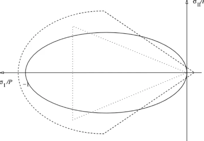
Fig. 2.The three yield curves discussed in the text plotted in stress invariant space; the elliptic, the modified Coulombic and the granu-lar model’s yield curves, depicted as solid, dashed and dotted lines, respectively.
τw=ρwCdw|v−vw|(v−vw), (6)
whereCdw andCda are drag coefficients,ρwandρaare air and water densities andvwandvaare the near surface water and wind velocities. This assumes that the wind velocity is much larger than the ice velocity; i.e. that|v−va|≈|va|.
The last term in Eq. (4) is the force due to the divergence of the internal stress tensorσ. Stress and strain rate (and thus ice velocity) are related through the sea-ice rheology. The three rheologies tested here are those suggested by Hibler (1979), Tremblay and Mysak (1997) and Hibler and Schul-son (2000), which are all isotropic viscous-plastic rheologies. In isotropic viscous-plastic models the relation between stress and strain can be represented using the stress invari-ants
σI =ζε˙I−P /2
σII =ηε˙II, (7)
whereζandηare the non-linear bulk and shear viscosities,ε˙I andε˙IIare the strain rate invariants andP is a pressure term. The viscosities,ζ andη, depend on the strain rate andP. We briefly describe each rheology here, but refer the reader to the original publications for more detail.
The rheology suggested by Hibler (1979) is by far the most commonly used viscous-plastic rheology. It uses an elliptical yield curve (see Fig. 2) and a normal flow rule. For typical strain rates, plastic flow occurs, while for very small strain rates the ice becomes linear viscous and enters so called “creep flow”. This creep flow occurs for all three yield curves at small strain rates. The pressure term is calculated via
P =P∗Ahexp(−C[1−A]), (8)
whereP∗ andC are constants, which must be chosen em-pirically. The elliptical yield curve reproduces basic sea-ice
characteristics, i.e. the ice is weak in tension, strong in shear and strongest in compression.
A different approach to the elliptic yield curve was sug-gested by Tremblay and Mysak (1997), who proposed a model based on a granular material rheology. This is equiv-alent to dynamic friction between two dry surfaces where the frictional shear force is proportional to the normal force. For stress ratios of shear force vs. normal force smaller than a given coefficient of friction the ice behaves like an elastic solid, while for larger stress ratios it flows like a fluid. The pressure term is found by perturbing the last known solu-tion to the momentum equasolu-tion so that the resulting veloc-ity field has a divergence determined by a given angle of dilation. This is done via an additional iterative solver and the numerical performance of the granular model is there-fore worse than that of the other two formulations. For pres-sure larger than the maximum, determined by Eq. (8), the ice compresses but otherwise behaves like an incompressible Newtonian fluid with non-linear shear viscosity. The bulk viscosity (ζ) is therefore always zero. For the granular model
P∗ in Eq. (8) is replaced with P∗/1.5 in accordance with Tremblay and Hakakian (2006). The resulting yield curve is a triangle (see Fig. 2).
Finally we include a yield curve which can be thought of as a combination of the other two. This is the so-called modified Coulombic yield curve, introduced by Hibler and Schulson (2000). Even though the term “modified Coulombic yield curve” (coined by Heil and Hibler, 2002) is used here, this yield curve is really a modification of the elliptic yield curve proposed by Hibler (1979). The curve gives friction-based failure up to a limiting compressive stress while the elliptic formulation holds for higher stresses. This limit is set at pure shear deformation, in accordance with the results of labo-ratory experiments. The pressure term is calculated using Eq. (8). The yield curve also includes a small amount of ten-sile stress. The resulting shape is elliptical for large stresses and triangular for small stresses (see Fig. 2).
The other main focus of this study is on the formulation of the new-ice thickness, which is expressed through the source/sink termSA in Eq. (3). The two methods for cal-culating SA considered, were formulated by Hibler (1979) and Mellor and Kantha (1989).
Hibler’s approach can be written as
ocean surface from its super-cooled state to freezing. When freezing1how>0 andSm>0 so that Eq. (9) becomes simply
SA=(1−A)1how/ h0. (10)
This means that the newly formed ice covers an areaSA so that its thickness is greater than or equal toh0.
The other approach to calculating SA considered here is the one originally proposed by Mellor and Kantha (1989). Based on an empirical formula by Nikiferov (1957) they for-mulateSAas
SA=8(1−A)
1how
h , (11)
where8is an empirically determined function. Mellor and Kantha (1989) differentiate between melting and freezing by giving8different constant values;
8=
8F=4 if1how>0
8M=0.5 otherwise. (12)
We can easily recover Eq. (10) from Eq. (11) by setting
8F=h/ h0, which givesh0=h/8F. Equation (11) therefore states that during freezing the newly formed ice will have a thickness equal toh/8F. In particular, this means that when ice forms in a grid cell that previously had no ice (i.e.h=0) this cell will become fully covered with ice with thickness
1how.
2.2 Control run
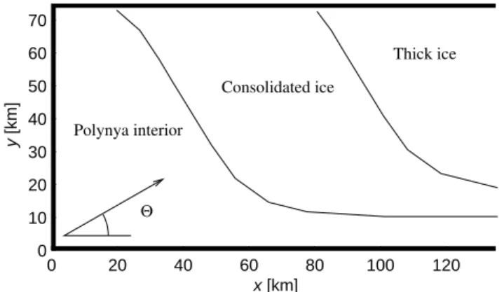
The model domain is a bay, 135 km long and 75 km wide at 2.5 km resolution (see Fig. 3), similar to the setup Bjornsson et al. (2001) used. At such a high resolution we must assume that on average the ice floes being modelled are no larger than 250 m in diameter. This is because a scale of approximately 10 grain widths can generally be modelled without resolv-ing each individual element usresolv-ing a granular model (Savage, 1998). McNutt and Overland (2003) state that at the multi-floe scale (approximately 2–10 km) sea ice behaves like a granular material, so the granular model should be ideal for a simulation at that scale. We can assume the ice floes in the polynya interior are no larger than pancake ice, which is not much larger than 3 m in diameter. The ice in the polynya in-terior, and by extension the consolidated ice, is therefore well within the maximum allowed floe size. However, assuming that individual floes are no larger than 250 m in diameter may not always be valid for the thick initial ice, depending on the geographical location of the polynya as well as the time of year. This is only a minor concern for this study since it fo-cuses on the steady state solution where the thick initial ice does not play a role (as it has drifted out of the model do-main).
A polynya is created by having a 15 m/s wind blow uni-formly at a 30◦ angle to the direction along the bay. The polynya forms at the bottom of the bay and the excess ice flows out the open boundary at the mouth of the bay. The
0 20 40 60 80 100 120
0 10 20 30 40 50 60 70
x [km]
y
[km]
Θ Polynya interior
Consolidated ice
Thick ice
Fig. 3.The size of the basin (in km) and wind direction during the polynya experiments. The figure also shows the three ice regimes one expects; the polynya interior (where the ice is in free drift), consolidated ice and thick initial ice.
atmospheric temperature is kept constant at Tair=−20◦C and the oceanic temperature is kept at the freezing point for a salinity ofS=32. The water velocity is always zero. The model is initialised with ice concentrationA=0.9 and thick-nessh=1 m. For the solid boundaries, a no-slip condition is used, while for the open boundary zero gradient Neumann boundary conditions are applied to all variables. The Neu-mann condition is also used for the ice pressureP, which Bjornsson et al. (2001) set to zero at the open boundary. This is done because using the Neumann condition improves the model behaviour near the open boundary by eliminating the excessive ice speed observed there by Bjornsson et al. (2001).
For the ice pressure constantsCandP∗in Eq. (8) we use the same values Bjornsson et al. (2001) used; i.e.C=30 and
P∗=30 kN/m2. Bjornsson et al. (2001) showed that these pa-rameters have little effect on the model results using the gran-ular model and we have found the same to be true for the other yield curves. A list of the relevant constants is included in Table 1.
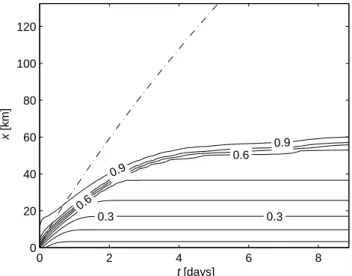
To illustrate the temporal evolution of the polynya, Fig. 4 shows a Hovm¨oller diagram of the ice concentration field taken along a section at y=37.5 km. The response to the applied wind stress is immediate and a discernible polynya edge starts to form during the first day of the model integra-tion. After two days the polynya has a clear structure and can be considered fully formed. A practically steady state has been reached after eight days. When the polynya has fully formed a band of large gradient in the concentration field analogous to the polynya edge always exists. For fur-ther reference Fig. 5 shows the ice concentration in the basin after eight days of model integration. As Figs. 4 and 5 show, the edge in this simulation is at a concentration of between
A=0.6 andA=0.9.
0.3 0.3
0.6
0.6 0.9
0.9
t [days]
x
[km]
0 2 4 6 8
0 20 40 60 80 100 120
Fig. 4. A Hovm¨oller diagram of the ice concentration field (A) in
the control experiment taken along a section aty=37.5 km. The
vertical axis (x) is the along-channel distance and the horizontal
axis (t) is the model time. The dash-dotted line shows theh=1 m
isoline separating the thick initial ice and consolidated ice.
x [km]
y
[km] 0.1
0.3 0.5
0.9
0.9
0.2
0.4
0 20 40 60 80 100 120
0 10 20 30 40 50 60 70
Fig. 5. Sea-ice concentration in the control experiment (A) after eight days of model integration. The polynya edge is visible as a sharp increase in concentration.
rate isF (A=0)=13.83 cm/day. In the polynya interior the ice is between 30 cm and 34 cm thick. If we assume all that ice is 32 cm thick we can calculate the ice formation rate in the polynya interior as a weighted average ofF (A=0)and
F (A=1, h=32cm)=3.31 cm/day; i.e.
F =AF (A=1, h=32 cm)+(1−A)F (A=0). (13) This approximation is correct to within 0.05 cm/day for
A.0.8, but starts breaking down as the consolidated ice gets thicker. Defining the polynya as all points for whichA<0.8 (this choice will be discussed further below), the mean ice formation rate in the polynya is F=11.1 cm/day after two days andF=10.7 cm/day after eight days.
According to Ou (1988), ice velocity in the model should fall into two categories; that of free drift in the polynya
Table 1.Main physical parameters and constants used in the simu-lation.
Variable Symbol Value
air drag coefficient Cda 1.2×10⁻³
air temperature Tair −20◦C
angle of dilatency δ 10◦C
basin dimensions L,W 135 km, 75 km
cloud cover Fc 80%
Coriolis factor f 1.33×10⁻⁴s−1
ellipse axis ratio e 2
horizontal resolution 1x 2.5 km
ice demarcation thickness h0 30 cm
ice density ρi 930 kg/m3
ice strength parameters C,P∗ 30, 30 kN/m2
internal angle of friction φ 30◦
min. viscosity (Hibler) ζmin 4×10⁸kg/s
relative humidity HR 80%
water drag coefficient Cdw 5.5×10⁻³
wind speed, angle |va|,2 15 m/s, 30◦
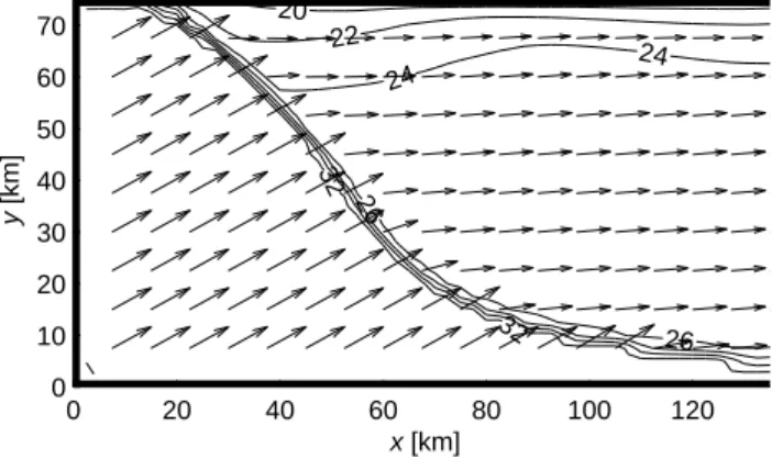
itself and that of the consolidated ice. In the dynamic-thermodynamic model this velocity change gives the ice drifting in the polynya interior a barrier of slower consol-idated ice to pile up against. Figure 6 shows the velocity field and speed in the control experiment after eight days. The speed does indeed fall into two categories: The free drift speed|vf|=32.6 cm/s and the speed of the consolidated ice|vc|.25 cm/s, depending on the distance away from the y=75 km boundary. More importantly the cross channel ve-locity,v, changes fromvf=15.7 cm/s tovc.3 cm/s in the con-solidated ice. Bjornsson et al. (2001) showed that it is the cross channel velocity that is most important for the size and shape of the polynya. In the polynya interior the ice drifts with the wind but the consolidated ice slides along the
y=75 km boundary with a small cross channel velocity com-ponent due to ridging at the boundary.
x [km]
y
[km]
20 22
24
24
26 26
32
32
0 20 40 60 80 100 120
0 10 20 30 40 50 60 70
Fig. 6. Ice velocity (v) and speed (|v|) in the control experiment after eight days of model integration. The polynya edge is visible as a sharp decrease in the ice velocity.
In the rheologies used here Eq. (8) dictates the ice strength under compression as a function of ice thickness and con-centration. When this term is small the rheology term be-comes small and the ice is in free drift. Since the ice in the polynya interior is in free drift we propose that the location of the polynya edge, in this particular setup, can be approxi-mated byA=0.8. This is becauseP (A=0.8)/P (A=1)≈0.01 so the rheology will play a negligible role at lower concen-trations. This choice is valid for the control run since the
A=0.8 contour is within the high gradient region where the polynya edge is found (see Fig. 5). It is also valid for all the following experiments done here, except when using a minimum on the bulk viscosity (ζ) and when using the new-ice thickness parametrisation of Mellor and Kantha (1989). These two cases will be discussed separately.
3 Different yield curves
An important part of the motivation for this study was to compare the results of Bjornsson et al. (2001), using the granular model, to a similar setup using different rheologies. The elliptic yield curve of Hibler (1979) is the most popular yield curve in use today, but it was designed for much lower resolution. It is therefore important to see how it fares in this high resolution setup. The modified Coulombic yield curve was, on the other hand, designed to model ice at high reso-lution so it will be instructive to see its performance here as well. In this section the focus is on the model response in the consolidated ice, since the rheology does not play a role inside the polynya itself.
In his model Hibler (1979) used a minimum for the bulk viscosity; ζmin=4×10⁸kg/s “in order to insure against any nonlinear instabilities” noting that that value is “several or-ders of magnitude below typical strong ice interaction val-ues and effectively yields free drift results” (Hibler, 1979, p. 823). The lower bound should only be necessary when the material derivative is included in the momentum Eq. (4) since
0 20 40 60 80 100 120
0 10 20 30 40 50 60 70
x [km]
y
[km]
granular ellipse mod. Coulomb
Fig. 7. The polynya edge (A=0.8) using the elliptic and modified Coulombic yield curves and the granular model after eight model days. The differences between different model formulations are mi-nor.
in that case having no lower bound will typically result in a noisy solution (Griffies and Hallberg, 2000). Most modern ice models ignore the material derivative and do not include a lower bound on ζ. However, as the resolution increases the material derivative becomes more important. The scaling argument made by Rothrock (1975) shows that the material derivative may need to be included as the shortest significant length scale becomes smaller than about 5 km.
In this idealised setup the material derivative has very little effect on the final solution, regardless of which rheology is used. The difference between the results with and without the material derivative is about 7 mm/s in the grid cells at the
x=0 boundary and about 2 mm/s at the y=75 km boundary and at the polynya edge. Everywhere else in the domain the difference is less than 0.1 mm/s. Compared to the free drift speed of |vf|=32.6 cm/s this is small. We also observe no noise, even when the material derivative is included and the lower bound onζ is set to zero.
Without a lower bound onζ the results using the elliptic yield curve are nearly identical to those using the granular model. There is a sharp transition from free drift ice to con-solidated ice, analogous to the polynya edge, just like in the granular model. This polynya edge forms at nearly the same location as it does in the granular model. Using the modified Coulombic yield curve also gives results very similar to the granular model. This is to be expected, since the modified Coulombic yield curve is in a way a combination of the other two yield curves. The difference between the three model formulations is limited to a small variance in polynya size, which as Fig. 7 shows, is due to a shift of the polynya edge by a few grid boxes. In particular, the commonly used el-liptic yield curve is sufficient and can be used safely in this context.
Using a minimum onζ does, however, give considerably different results from the control run. Setting the minimum to
0 20 40 60 80 100 120 0
10 20 30 40 50 60 70
x [km]
y
[km]
0.2
0.4 0.6
0.8
0.9
0.7
0.5
0.3
0 20 40 60 80 100 120
0 10 20 30 40 50 60 70
x [km]
y
[km]
25 25
25
20
20
20
15
10
15
10
Fig. 8.Sea-ice concentration (top) and speed and velocity (bottom) using Hibler’s original formulation for the elliptic yield curve, after eight days of model integration. Neither figure shows a discernible
polynya edge. The dash-dotted line shows the isoline forA=0.8
from the control run.
with a very diffuse edge, as Fig. 8 shows. Speed and veloc-ity also fail to meet the criteria for forming a polynya edge; i.e. there is no clear separation between the velocity of the ice in the polynya interior and consolidated ice (see Fig. 8). In addition, the ice in the polynya interior does not flow at a con-stant speed and its speed is sometimes lower than that of the consolidated ice, which is clearly not plausible. The speed of the ice in the polynya interior when usingζmin=4×10⁸kg/s is also always lower than it is in the control run. A decrease in the ice concentration is also seen by they=75 km boundary, contrary to what can be seen in the control run. These effects were noted by Hunke (2001) in a different setup, but that discussion focused on the effects seen at the solid boundary, which will not be discussed further here.
The polynya edge becomes so diffuse because when im-posing such a high minimum onζ, the viscosity is consis-tently kept at its minimum value forA.0.9 throughout the simulation. This is because the viscosity is related to the ice pressure via
ζ =P /21 and η=ζ /e2, (14)
and the pressure to ice concentration via Eq. (8). The flow whereAis sufficiently small is therefore linear viscous, but choosing as a minimumζmin=4×10⁸kg/s does not result in
effectively free drift. Lu et al. (1989) also found that this limit was too high compared to measurements.
As previously stated, we observed no non-linear insta-bilities using ζmin=0 kg/s. Some noise is, however, to be expected in a realistic simulation and so a non-zero ζmin may be required if one wants to include the material deriva-tive. In that case one would need to choose a low, but non-zero value forζmin. The resolution of Hibler’s model was 125 km and since viscosity scales with the distance squared, a choice ofζmin=4×10⁴kg/s seems in order. This yields nearly the same results as with ζmin=0 kg/s; the largest difference in concentration between the two model runs being 1A=0.006. The maximum concentration gra-dient when using ζmin=0 is max(|∇A|)=0.230 km−1 and it is max(|∇A|)=0.228 km−1 when usingζmin=4×10⁴kg/s. When choosing larger values forζmin, the effects of the cap-ping start to show. Forζmin=4×10⁵kg/s the maximum gra-dient is max(|∇A|)=0.212 km−1 and the difference in con-centration between that run and the one with zero ζmin is
1A=0.08. For ζmin=4×10⁶kg/s the maximum gradient is max(|∇A|)=0.164 km−1and the concentration difference is
1A=0.3.
4 New-ice thickness
As we have already seen, the ice rheology affects the ini-tial ice pack and the consolidated ice. The interior of the polynya, on the other hand, is primarily affected by the new-ice thickness parametrisation. This determines the thick-ness, and thus the concentration of the ice formed inside the polynya.
The most popular method for parametrising the new-ice thickness is probably the one suggested by Hibler (1979) (see Sect. 2.1). Put simply the new-ice thickness is not allowed to drop below a certain minimum,h0. If the total mass of newly formed ice is not enough to cover the open water fraction of the grid cell at that thickness then the concentration of newly formed ice is adjusted accordingly. If more ice is formed then the new ice is simply thicker thanh0.
The choice ofh0is not obvious and appears to range from 10 to 50 cm or even more in some cases. Bjornsson et al. (2001) argued for usingh0=30 cm and that is the value used here so far. Their argument is based on the assumption that the ice that forms in the polynya immediately forms pancake ice. However, Bjornsson et al. (2001) state that pancake ice thickness is closer to 10 cm than 30 cm. We therefore include a model run withh0=10 cm.
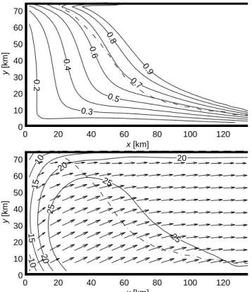
The main result of using h0=10 cm is that with a lower
0 20 40 60 80 100 120 0
10 20 30 40 50 60 70
x [km]
y
[km]
0.2
0.4 0.6
0.7 0.5 0.3
0.8 0.9
0.9
0 20 40 60 80 100 120
0 10 20 30 40 50 60 70
x [km]
y
[km]
32 32
30
28 28
26
26
24
24
22 20
Fig. 9.The ice concentration (A, top) and speed and velocity (vand
|v|, bottom) usingh0=10 cm after eight model days. The resulting
polynya is smaller and has a higher ice concentration than the
con-trol run. The dash-dotted line shows the isoline forA=0.8 from the
control run.
concentration field as when usingh0=30 cm. It is, however, still sharp in the velocity field, as can be seen in Fig. 9.
The mean ice formation rate in the polynya is about 1% lower here than in the control run. The total ice formation is therefore reduced almost only because the polynya is smaller. Using h0=30 cm gives polynya area of Ap=4.5×10³km2 after eight days, but using h0=10 cm the polynya area is
Ap=2.4×10³km2after eight days; an approximately 50% re-duction in size. Finally, the consolidated ice is thinner since its thickness equalsh0.
The other approach to determining the thickness of newly formed ice described in Sect. 2.1 is the one proposed by Mel-lor and Kantha (1989). There the thickness of newly formed ice is based on the thickness of the ice already present in the grid cell. Mellor and Kantha (1989) argued that the thick-ness of newly formed ice should be a quarter of the old ice thickness. This also means that when there is no ice in the grid cell when new ice forms, the ice spreads uniformly over the entire cell, potentially very thinly. A polynya in such a model may therefore be hard to recognise by the change in concentration and researchers using this approach often con-sider ice below a certain cut-off thickness to represent the polynya. Smedsrud et al. (2006), for instance, useAh=30 cm for this cut-off thickness.
0 20 40 60 80 100 120
0 10 20 30 40 50 60 70
x [km]
y
[km]
0.9
0.9
0.9
0.8
0.8
0 20 40 60 80 100 120
0 10 20 30 40 50 60 70
x [km]
y
[km]
30
30
28 28 28 26
26 24
24 22 22
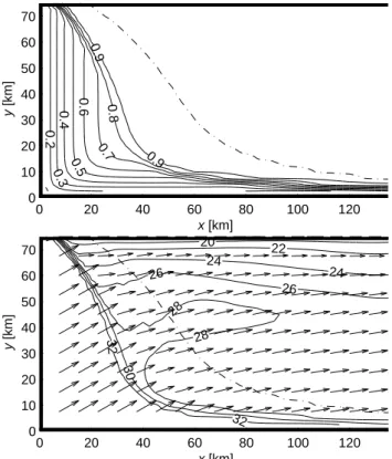
Fig. 10. The ice concentration (A, top) and speed and velocity
(vand|v|, bottom) using the new-ice thickness parametrisation by
Mellor and Kantha (1989) after eight model days. The resulting polynya is very small with no discernible edge in the velocity field.
The dash-dotted line shows the isoline forA=0.8 from the control
run.
Using this approach results in a “polynya” that is hardly recognisable in the concentration field, as Fig. 10 shows. Even after eight days there is only a thin sliver of an open-ing along thex=0 km andy=0 km boundaries and theA=0.8 isoline is a grid box or two away from the shore. More seri-ously perhaps the velocity field, also shown in Fig. 10, shows no sign of the discontinuity deemed necessary for proper polynya formation. The ice slows down gradually moving away from the x=0 boundary, contrary to our previous as-sumptions about how a polynya is formed.
Ice thickness near the coast is indeed lower than the initial ice thickness, but as Fig. 11 shows there is no real polynya edge to be found in the ice thickness field. In that respect there is no conceptual difference between usinghorAh. As before the thick initial ice drifts out of the basin, but in this case the ice that replaces it does not have a uniform thickness. It is very thin at the coast with linearly increasing thickness towards the thick initial ice.
0.3
0.3
0.3
0.6
0.6
0.9
0.9
t [days]
x
[km]
0 2 4 6 8
0 20 40 60 80 100 120
Fig. 11. A Hovm¨oller diagram of the ice thickness field (h) us-ing the new-ice thickness formulation by Mellor and Kantha (1989)
taken along a section aty=37.5 km. The vertical axis (x) is the along
channel distance and the horizontal axis (t) is the model time. The
dash-dotted line shows the isoline forA=0.8 from the control run.
0 20 40 60 80 100 120
0 10 20 30 40 50 60 70
10
10
x [km]
y
[km]
20
20 30 30
h
0 = 30 cm variable h0
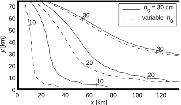
Fig. 12.The polynya edge after eight days using a constanth0and
parametrisedh0according to Eq. (15). A=0.8 is used as a marker
for the polynya edge and the edge is plotted for 10, 20 and 30 m/s wind speed.
The parametrisation by Winsor and Bj¨ork (2000) lends itself well to immediate inclusion in the dynamic-thermodynamic model. It is based only on the wind speed and not the polynya width, frazil ice speed or other quan-tities not accessible to the dynamic-thermodynamic model. By using this parametrisation we aim at improving the mod-elled consolidated ice thickness and thus also the size of the polynya.
Winsor and Bj¨ork (2000) assumed the collection depth to be a function of wind speed as
H=a+ |va|b
c , (15)
10 15 20 25 30 35
0 1 2 3 4 5 6 7 8
|va| [m/s]
A p
[10
3 km 2 ]
h0 = 30 cm
h0 = 10 cm
variable h0
Fig. 13. The polynya size (Ap) after eight days as a function of
wind speed (|va|). The size is calculated as the sum of the size of
all model points whereA<0.8.
where|va|is the surface wind velocity, a=1 m,b=0.1 s and
c=15. In particular, H≈7 cm for |va|=0 and H=30 cm for |va|=35 m/s so this parametrisation is well within the range of plausible values forh0. Equation (15) is then used to cal-culateh0=Hin each grid point.
Using this parametrisation results in smaller polynyas at low wind speeds, compared toh0=30 cm or larger polynyas at high wind speeds, compared to h0=10 cm. Figure 12 shows the polynya usingh0=30 cm and the parametrisation for the wind speeds 10, 20 and 30 m/s. At lower winds the polynya edge starts to become diffuse, which is to be ex-pected. For further reference Fig. 13 shows the size of the resulting polynya as a function of wind speed. The mean ice formation rate in the polynya increases fromF=10 cm/day for|va|=10 m/s toF=11 cm/day for|va|=35 m/s and choos-ing different values for h0 contributes to about 1% change in the ice formation rate. At the same time the polynya size grows approximately four times as the wind strength grows from 10 m/s to 35 m/s. It is therefore clear that variations in polynya size control the variations in total ice formation in the polynya.
5 Discussion
computing time the other two rheologies require. The elliptic yield curve of Hibler (1979) is also already in use in the vast majority of sea-ice models.
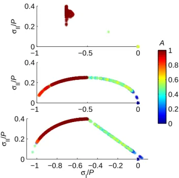
All three yield curves give nearly identical results (with the exception of using a cappedζ as discussed below). Looking at the stress states (Fig. 14) we see that when using the gran-ular model theσIvalues for points in the consolidated ice are all clustered aroundσI=−P /1.5. This means that at these points the ice cover yields or is very close to yielding under compression. When this is the case the behaviour of the ice is controlled by Eq. (8), which is also one of the main equa-tions governing the behaviour of the other two yield curves. The difference between the granular model and the other two is then almost entirely explained by the different formulation of shear strength between the model formulations. As Fig. 2 shows, the granular model and the ellipse have a lower shear strength than the modified Coulombic yield curve, which is why using the modified Coulombic yield curve gives a smaller polynya.
Using the other two yield curves, the stress states are much more evenly distributed along the σI axis. For the modi-fied Coulombic yield curve the stress states that lie on the Coulombic slope are all inside the polynya while the stress states in the consolidated ice are all on the elliptic part of the yield curve. This happens because in the consolidated ice the divergence (ε˙) is always negative, so according to Eq. (7)
σI≤−P /2. Using the elliptic and modified Coulombic yield curves therefore yields similar results for the consolidated ice, where both yield curves have an elliptic shape. In the polynya interior the ice is in free drift so the shape of the yield curve has no effect there.
Using a largeζmin, in particularζmin=4×10⁸kg/s as Hibler (1979) suggests, does, however, give results that are not plau-sible. Using this original formulation results in a polynya that is smeared out with no proper edge and a velocity field that has little relation to polynya formation. This happens be-cause the capping ofζ in the model turns the viscous-plastic formulation into a linear viscous model for ice concentration
A<0.9.
Hibler (1979) used the lower bound onζ to dampen grid scale noise which can arise when the grid Reynolds number constraint is not satisfied. Considering the limited case of Burger’s equation in one dimension:
dv
dt +v
dv
dx =A
d2v
dx2, (16)
A must be bounded by A>12v1x (Griffies and Hallberg, 2000). In free drift and ignoring the sea surface tilt term, the momentum equation becomes Burger’s equation and for the one dimensional caseA=ζ /ρi. Using the free drift speed of |vi|=32.6 cm/s and 1x=2.5 km the viscosity is bounded by
ζ >12ρi|vi|1x≈4×10⁵kg/s.
The grid Reynolds number constraint is therefore an or-der of magnitude larger than our preferred value for a non-zeroζmin. Since ignoring the material derivative had much
−10 −0.5 0
0.2 0.4
σ II
/P
−10 −0.5 0
0.2 0.4
σ II
/P
−1 −0.8 −0.6 −0.4 −0.2 0
0 0.2 0.4
σ II
/P
σI/P
A
0 0.2 0.4 0.6 0.8 1
Fig. 14. Stress states using the granular model (top), the elliptic yield curve (centre) and modified Coulombic yield curve (bottom) after eight model days plotted in stress invariant space. The colour scale indicates the ice concentration at each point (A) and points with high concentration are drawn on top of those with a lower
con-centration. Points with high values ofA(A&0.8) are all located in
the regionσI≤−P /2. Points near the open boundary are excluded
from the figure.
less effects on the simulation than using a non-zeroζminwe conclude that ignoring the material derivative is preferable to including it and a non-zeroζmin.
With regards to the ice behaviour inside the polynya we considered three ways in which to parametrise the thickness of ice forming over open water. These are the methods sug-gested by Hibler (1979), Mellor and Kantha (1989) and an adaptation of the collection depth parametrisation by Winsor and Bj¨ork (2000). Hibler’s method was used when investi-gating the dynamic aspects (Sect. 3) with an ice demarca-tion thicknessh0=30 cm after Bjornsson et al. (2001). That value may be too high and so we also ran the model using
h0=10 cm.
Using a lowerh0resulted in a smaller polynya but little change in mean ice formation rates (about 1%). The ice con-centration in the polynya interior was higher and as a result the concentration field did not show a sharp polynya edge. The velocity field, on the other hand, still showed a clear dis-continuity at the polynya edge. The width of the polynya did decrease, but that was to be expected and can be understood in relation to the Lebedev-Pease width of a polynya (Pease, 1987)
L=H U
whereLis the polynya width andHUis the flux of consoli-dated ice. The collection depth,H, is analogous toh0in the dynamic-thermodynamic model. Loweringh0from 30 cm to 10 cm results in approximately 1% reduction in the ice for-mation rate (F). The polynya width is therefore bound do decrease.
Results obtained using the formulation of Mellor and Kan-tha (1989) were, however, very different from those obtained in the control run. Using Mellor and Kantha’s formula-tion there are two ice regimes; thick ice and thin ice, which may be characterised as nilas. This replaces the threefold separation of thick ice, consolidated ice (of uniform thick-ness) and frazil/free drift ice, seen in polynya flux models and the control run. The polynya edge is considered to be what separates the consolidated ice and frazil/free drift ice, but this distinction is lost when using the Mellor and Kantha (1989) approach. The new-ice thickness formulation by Mel-lor and Kantha (1989) is therefore not suitable for modelling polynyas.
On the whole, the approach by Hibler (1979) is also more reasonable from a physical standpoint. This is because wind and waves, which cannot be resolved by ocean or atmosphere models, will transform the frazil ice in the polynya into pan-cake ice, similar to the ice formation in that scheme. What is unrealistic about Hibler’s approach is that solid ice forms inside the polynya, even where in reality the ice is mainly frazil ice. The thin ice formed using Mellor and Kantha’s approach is more akin to grease ice or nilas which form in calmer conditions.
Wind speed is therefore an important factor in determining the new-ice thickness and it is consequently an important part of collection depth parametrisations for polynya flux models. Winsor and Bj¨ork (2000) parametrised the collection depth in the Pease (1987) model based only on wind speed and we found that parametrisation easily adoptable for inclusion in the dynamic-thermodynamic model.
Using the Winsor and Bj¨ork (2000) parametrisation gives results in the range between the results when using a constant
h0=10 cm andh0=30 cm. We have already expressed a pref-erence for the Hibler (1979) parametrisation for the new-ice thickness and using the Winsor and Bj¨ork (2000) parametri-sation enables us to choose a sensible value for h0. As a result the polynya size should depend on wind strength in a more realistic manner than when using a constanth0. Using the parametrisation should also give more realistic ice thick-ness for the consolidated ice.
On a more general note, such a small value forh0may not be suitable for models describing the central pack ice as well. In such a situation the approach of Mellor and Kantha (1989) may give better results since the thick pack ice appears to require a largerh0.
It is trivial to combine all three approaches to new-ice thickness parametrisation discussed here into one:
h0=max
h
8,
a+ |va|b c
, (18)
with8=4, a=1 m, b=0.1 s andc=15, as before. This ap-proach modifies the previously constanth0of Hibler (1979) so that for thick ice the approach of Mellor and Kantha (1989) is used and for thinner ice the parametrisation of Win-sor and Bj¨ork (2000) is used. Using one value for thick ice and one for thin is appropriate sinceh0is only analogous to the collection depth in a polynya or the marginal ice zone. Where the ice is thicker the ice behaviour should be simi-lar to that described by Mellor and Kantha (1989), given the empirical origin of their formulation.
In our setup the result of Eq. (18) will always be the same as that of Eq. (15) since the ice in the polynya is always thin in the sense thath<8(a+|va|b)/c. Further testing of this new parametrisation can therefore not be done here but should be carried out in a realistic simulation.
In conclusion we note that in this idealised setup the polynya is best defined as the area where A<0.8. This is really the concentration where the ice behaviour starts chang-ing from free drift, forA.0.8, to being heavily influenced by internal stresses, forA≈1. This separation is based on Eq. (8) and on the choice ofC. TheA=0.8 isoline is also consistently within the high gradient region forAin all experiments, ex-cept when using too high a minimum for the bulk viscosity and when using the new-ice thickness parametrisation from Mellor and Kantha (1989). But both these cases were found to give implausible results.
6 Conclusions
We have used an idealised setup to test three different sea-ice rheologies and three different formulations for the thickness of newly formed ice during polynya formation. These tests were done using a dynamic-thermodynamic sea-ice model in an idealised channel, similar to what Bjornsson et al. (2001) did.
We were able to reproduce the results of the granular model using both the modified Coulombic yield curve of Hibler and Schulson (2000) and the elliptic yield curve of Hibler (1979). This is important, since the numerical per-formance of the granular model is substantially worse than that of the other two models and also since the elliptic yield curve is already in popular use. We also found that including the material derivative and setting a minimum on the bulk viscosity is not a viable alternative to ignoring the material derivative.
concentration and velocity field. We conclude therefore that this approach does not enable us to properly model polynyas. Hibler’s approach, on the other hand, gave a clear separation of the consolidated ice and the polynya itself.
Using Hibler’s new-ice thickness parametrisation and any of the rheologies tested here should give realistic results when modelling polynyas. Polynyas that are fully resolved by the model grid can then be recognised as areas of low concentration enclosed by compact ice and/or land. We also suggest usingA<0.8 as a criterion for low concentration.
Hibler (1979) assumed a constant demarcation thickness (h0). We suggest, however, using the collection thickness parametrisation of Winsor and Bj¨ork (2000) to parametrise
h0. This results in a value for h0 which is dependent on wind strength and in the range already deemed acceptable forh0. As an aside, a combination of this parametrisation with the approach of Mellor and Kantha (1989) is proposed. This should give a parametrisation forh0applicable for both the marginal ice zone and the central ice pack.
Acknowledgements. We would like to thank Dirk Notz for his thorough reading of the manuscript and helpful suggestions and Bruno Tremblay for useful discussions during the course of this work. We would also like to thank Stefan Heitmann for his help during the development of the ice model. Finally we would like to thank the two anonymous reviewers for their comments, which helped to greatly improve the quality of the manuscript. This work was financed by the DFG under HA 3166/2-1 “STARBUG”.
Edited by: S. Marshall
References
Backhaus, J.: Improved representation of topographic effects by a vertical adaptive grid in vector-ocean-model (VOM), Part I: Generation of adaptive grids, Ocean Model., 22, 114–127, doi: 10.1016/j.ocemod.2008.02.003, 2008.
Bjornsson, H., Willmott, A. J., Mysak, L. A., and
Morales Maqueda, M. A.: Polynyas in a high-resolution
dynamic-thermodynamic sea ice model and their parame-terization using flux models, Tellus, 53A, 245–265, doi: 10.1034/j.1600-0870.2001.00113.x, 2001.
Coon, M. D., Maykut, G. A., Pritchard, R. S., Rothrock, D. A., and Thorndike, A. S.: Modeling the pack ice as an elastic-plastic material, AIDJEX Bulletin, 24, 1–105, 1974.
Griffies, S. M. and Hallberg, R. W.: Biharmonic friction
with a Smagorinsky-like viscosity for use in large-scale eddy-permitting ocean models, Mon. Weather Rev., 128, 2935–2946, doi:10.1175/1520-0493(2000)128h2935:BFWASLi 2.0.CO;2, 2000.
Harms, I., H¨ubner, U., Backhaus, J. O., Kulakov, M., Stanovoy, V., Stepanets, O., Kodina, L., and Schiltzer, R.: Salt intrusions in Siberian river estuaries: Observations and model experiments in Ob and Yenisei, in: Siberian River Runoff in the Kara Sea: Characterization, Quantification, Variability and Environmental Significance, no. 6 in Proceedings in Marine Science, pp. 27–46, Elsevier, 2003.
Heil, P. and Hibler, III, W. D.: Modelling the High-Frequency Components of Arctic Sea Ice Drift and Deformation, J. Phys. Oceanogr., 32, 3039–3057, doi:10.1175/1520-0485(2002) 032h3039:MTHFCOi2.0.CO;2, 2002.
Hibler III, W. D.: A Dynamic Thermodynamic Sea Ice Model, J. Phys. Oceanogr., 9, 815–846, doi:10.1175/1520-0485(1979) 009h0815:ADTSIMi2.0.CO;2, 1979.
Hibler III, W. D. and Schulson, E. M.: On modeling the anisotropic failure and flow of flawed sea ice, J. Geophys. Res., 105, 17105– 17120, doi:10.1029/2000JC900045, 2000.
Hunke, E. C.: Viscous-plastic sea ice dynamics with the EVP model: Linearization issues, J. Comput. Phys., 170, 18–38, doi: 10.1006/jcph.2001.6710, 2001.
Kern, S., Harms, I., Bakan, S., and Chen, Y.: A comprehensive view of Kara Sea polynya dynamics, sea-ice compactness and export from model and remote sensing data, Geophys. Res. Lett., 32, L15501, doi:10.1029/2005GL023532, 2005.
Lu, Q.-M., Larsen, J., and Tryde, P.: On the Role of Ice Interaction due to Floe Collisions in Marginal Ice-Zone Dynamics, J. Geo-phys. Res., 94, 14525–14537, doi:10.1029/JC094iC10p14525, 1989.
Marsland, S. J., Bindoff, N. L., Williams, G. D., and Budd, W. F.: Modeling water mass formation in the Mertz Glacier Polynya and Ad´elie Depression, East Antarctica, J. Geophys. Res., 109, C11003, doi:10.1029/2004JC002441, 2004.
Maykut, G. and Perovich, D.: The role of shortwave radiation in the summer decay of a sea ice cover, J. Geophys. Res., 92, 7032– 7044, doi:10.1029/JC092iC07p07032, 1987.
Maykut, G. A.: Large-Scale Heat Exchange and Ice Production in the Central Arctic, J. Geophys. Res., 87, 7971–7984, doi: 10.1029/JC087iC10p07971, 1982.
Maykut, G. A. and McPhee, M. G.: Solar heating of the Arctic mixed layer, J. Geophys. Res., 100, 24691–24703, 1995. McNutt, S. L. and Overland, J. E.: Spatial hierarchy in Arctic sea ice
dynamics, Tellus, 55, 181–191, doi:10.1034/j.1600-0870.2003. 00012.x, 2003.
McPhee, M. G.: Ice-ocean momentum transfer for the AIDJEX ice model, AIDJEX Bulletin, 29, 93–111, 1975.
Mellor, G. L. and Kantha, L.: An Ice-Ocean Coupled
Model, J. Geophys. Res., 94, 10937–10954, doi:10.1029/ JC094iC08p10937, 1989.
Morales Maqueda, M. A., Willmott, A. J., and Biggs, N. R. T.: Polynya dynamics: A review of observations and modeling, Rev. Geophys., 42, RG1004, doi:10.1029/2002RG000116, 2004. Nikiferov, E. G.: Variations in ice cover compaction due to its
dy-namics, in: Problemy Arktiki, vol. 2, Morskoi Transport Press, Leningrad, USSR, 1957.
Ou, H. W.: A time-dependent model of a coastal polynya, J. Phys. Oceanogr., 18, 584–590, doi:10.1175/1520-0485(1988) 018h0584:ATDMOAi2.0.CO;2, 1988.
Pease, C. H.: The size of wind driven polynyas, J. Geophys. Res., 92, 7049–7059, doi:10.1029/JC092iC07p07049, 1987.
Rothrock, D. A.: Steady Drift of an Incompressible
Arc-tic Ice Cover, J. Geophys. Res., 80, 387–397, doi:10.1029/ JC080i003p00387, 1975.
Savage, S. B.: Analyses of slow high-concentration flows of
Smedsrud, L. H., Budgell, W. P., Jenkins, A. D., and Adlandsvik, B.: Fine-scale sea-ice modelling of the Storfjorden polynya, Svalbard, Ann. Glaciol., 44, 73–79, 2006.
Tremblay, L.-B. and Hakakian, M.: Estimating the sea ice com-pressive strength from satellite-derived sea ice drift and NCEP reanalysis data, J. Phys. Oceanogr., 36, 2165–2172, doi:10.1175/ JPO2954.1, 2006.
Tremblay, L.-B. and Mysak, L. A.: Modeling Sea Ice as a Granular Material, Including the Dilatancy Effect, J. Phys. Oceanogr., 27, 2342–2360, doi:10.1175/1520-0485(1997)027h2342:MSIAAGi 2.0.CO;2, 1997.
Willmott, A. J., Morales Maqueda, M. A., and Darby, M. S.: A model for the influence of wind and oceanic currents on the size of a steady state latent heat coastal polynya, J. Phys. Oceanogr., 27, 2256–2275, doi:10.1175/1520-0485(1997) 027h2256:AMFTIOi2.0.CO;2, 1997.