Variational data assimilation with superparameterization

(1)

NPGD

2, 513–536, 2015

Variational data assimilation with

su-perparameterization

I. Grooms and Y. Lee

Title Page

Abstract Introduction

Conclusions References

Tables Figures

◭ ◮

Back Close

Full Screen / Esc

Printer-friendly Version Interactive Discussion

Discussion

P

a

per

|

Discussion

P

a

per

|

Discussion

P

a

per

|

Discussion

P

a

per

|

Nonlin. Processes Geophys. Discuss., 2, 513–536, 2015 www.nonlin-processes-geophys-discuss.net/2/513/2015/ doi:10.5194/npgd-2-513-2015

This discussion paper is/has been under review for the journal Nonlinear Processes in Geophysics (NPG). Please refer to the corresponding final paper in NPG if available.

Variational data assimilation with

superparameterization

I. Grooms and Y. Lee

Center for Atmosphere Ocean Science, Courant Institute of Mathematical Sciences, New York University, New York, USA

Received: 9 March 2015 – Accepted: 10 March 2015 – Published: 20 March 2015

Correspondence to: I. Grooms (grooms@cims.nyu.edu)

(2)

NPGD

2, 513–536, 2015

Title Page

Tables Figures

◭ ◮

Back Close

Full Screen / Esc

Discussion

P

a

per

|

Discussion

P

a

per

|

Discussion

P

a

per

|

Discussion

P

a

per

|

Abstract

Superparameterization (SP) is a multiscale computational approach wherein a large scale atmosphere or ocean model is coupled to an array of simulations of small scale dynamics on periodic domains embedded into the computational grid of the large scale model. SP has been successfully developed in global atmosphere and climate models, 5

and is a promising approach for new applications. The authors develop a 3D-Var varia-tional data assimilation framework for use with SP; the relatively low cost and simplicity of 3D-Var in comparison with ensemble approaches makes it a natural fit for relatively expensive multiscale SP models. To demonstrate the assimilation framework in a sim-ple model, the authors develop a new system of ordinary differential equations similar 10

to the two-scale Lorenz-’96 model. The system has one set of variables denoted{Yi},

with large and small scale parts, and the SP approximation to the system is straightfor-ward. With the new assimilation framework the SP model approximates the large scale dynamics of the true system accurately.

1 Introduction

15

Superparameterization (SP) is a multiscale computational method for parameterizing small scale effects in large scale atmosphere and ocean models. It was originally de-veloped and has been particularly effective as a cloud parameterization in atmosphere models (Grabowski and Smolarkiewicz, 1999; Randall et al., 2003), and has been im-plemented in global atmosphere and climate models (Khairoutdinov and Randall, 2001; 20

Tao et al., 2009; Randall et al., 2013). SP couples a large scale, low resolution model to an array of local small scale, high resolution simulations embedded within the com-putational grid of the large scale model. The comcom-putational cost is kept down through a variety of methods, most prominently by reducing the dimensionality of the small scale simulations, e.g. using one vertical and one horizontal coordinate in the afore-25

mentioned atmospheric applications. Although atmosphere and climate models with

(3)

NPGD

2, 513–536, 2015

Title Page

Tables Figures

◭ ◮

Back Close

Full Screen / Esc

Discussion

P

a

per

|

Discussion

P

a

per

|

Discussion

P

a

per

|

Discussion

P

a

per

|

SP are particularly successful at producing a realistic Madden–Julian oscillation and diurnal cycle of convection over land (Khairoutdinov et al., 2005), there are as yet no data assimilation systems designed for use with these models.

The authors recently developed an ensemble Kalman filter framework for data assim-ilation with SP (Grooms et al., 2014, hereafter GLM14). This framework was developed 5

in the context of stochastic SP, a variant of SP that reduces computational cost by re-placing the small scale simulations of SP with quasilinear stochastic models (Grooms and Majda, 2013; Majda and Grooms, 2014). Stochastic SP has only been developed for idealized turbulence models (Grooms and Majda, 2013, 2014a, b; Grooms et al., 2015), and is not yet implemented in global atmosphere, ocean, or climate models. 10

Because of the relatively high cost and computational complexity of global atmosphere and climate models with SP, the extra cost associated with an ensemble-based data assimilation system makes it unlikely that it will be possible to use these models with the framework of GLM14 in the near future.

Here we develop a 3D-Var variational data assimilation framework for SP that builds 15

on and modifies the framework of GLM14. Observations of physical variables have large scale and small scale parts, the former of which is equated with the large scale model variables, and the latter with the variables of the small scale embedded simula-tions. A key feature of SP is that the small scale simulations are periodic, so a location on the small scale computational grid does not correspond precisely to any location in 20

the real physical domain; as a result, the small scale simulations provide only statisti-cal information about the small sstatisti-cales, and this information can be used as a prior in the data assimilation context. In GLM14 an ensemble of SP simulations provides prior information on the large scale variables, but in the present approach the prior informa-tion on the large scales comes from a single SP simulainforma-tion and a time-independent 25

(4)

NPGD

2, 513–536, 2015

Title Page

Tables Figures

◭ ◮

Back Close

Full Screen / Esc

Discussion

P

a

per

|

Discussion

P

a

per

|

Discussion

P

a

per

|

Discussion

P

a

per

|

the observation operator is nonlinear the large and small scale analysis must be com-puted simultaneously by minimizing an objective function. Although analysis estimates of the small scale variables can be computed with linear observations, and must be computed with nonlinear observations, our framework does not at this time use the small scale analysis estimate to update any of the small scale SP variables because 5

the latter cannot be unambiguously associated with any real physical location. A key update of the GLM14 framework is that we here compute a small scale analysis es-timate at locations where observations are available, rather than at every coarse grid point. This can result in significant computational savings in the case of a nonlinear observation operator. We also update the GLM14 framework to better handle observa-10

tions at locations offthe coarse grid.

The 3D-Var framework with SP is presented in Sect. 2. In Sect. 3 we develop a new system of ODEs based on the two-scale Lorenz-’96 (L96) model (Lorenz, 1996, 2006), and an SP approximation to that system. Assimilation experiments using the new 3D-Var framework and the new system are described in Sect. 4, followed by conclusions. 15

2 Variational data assimilation with superparameterization

The key aspect of the GLM14 framework is the way in which the variables of the true dynamical system are related to those of the superparameterization. Let the large scale variables of the SP simulation be denotedu(the overbar does not denote a statistical mean), and let the small scale variables be denotedeu. In most SP applications there is 20

a set of small scale variables at every point of the large scale computational grid. The small scale variables exist on a local periodic domain, and have zero average across the periodic directions.

In GLM14, observations are related to the SP model variables using the following observation model

25

v₌H(L(u₊u′))+ε (1)

(5)

NPGD

2, 513–536, 2015

Title Page

Tables Figures

◭ ◮

Back Close

Full Screen / Esc

Discussion

P

a

per

|

Discussion

P

a

per

|

Discussion

P

a

per

|

Discussion

P

a

per

|

whereH is the observation operator and ε is a vector of zero-mean normal random variables associated with observation error. The vector u′ has the same size as u, and models the small-scale contribution to physical variables at the coarse grid points, i.e.u=u+u′is the vector of real physical variables at the coarse model grid points. The physical variablesuare interpolated to the location of the observations byL. The mean 5

and covariance ofu′ are computed from the statistics of the small scale SP variables e

u.

As noted in GLM14, it is unrealistic to use the same interpolation operator for both the large and small scale variables because it assumes that the small scale variables vary smoothly between the coarse grid points, whereas the small scale variables should by 10

definition vary over shorter distances. (Observations in GLM14 were taken only on the coarse grid points, avoiding the issue.) Instead of specifying an alternative interpolation operator for the small scales, we update the framework by altering the definition ofu′

to include small scale variables only at the points where observations are taken. LetP denote the number of different physical locations where observations are avail-15

able (for simplicity of exposition we assume that there is only one observation per lo-cation, i.e.v ∈RP). The updated observation model for thepth location is

vp=Hp(Lp(u)+u′p)+εp (2)

where L_p interpolates the large scale model variables u to the observation location and ε_p is a zero-mean Gaussian random variable. There is thus one vector u′_p of 20

small scale variables per observation location. The updated observation model for all

P observations can be written in vector form as

v₌H(L(u)+u′)+ε (3)

whereu′is no longer defined as in GLM14, but according to the discussion above. To complete the specification of the 3D-Var framework we specify a prior joint distri-25

bution foruandu′with mean

(6)

NPGD

2, 513–536, 2015

Title Page

Tables Figures

◭ ◮

Back Close

Full Screen / Esc

Discussion

P

a

per

|

Discussion

P

a

per

|

Discussion

P

a

per

|

Discussion

P

a

per

|

and covariance

B 0

0 P′

. (5)

The small scale variableu′is assumed to be uncorrelated with the large scale variable. In practice, the large and small scale variables are certainly not independent, but as shown in GLM14 the assumption that they are uncorrelated is reasonable. As typical 5

in a 3D-Var setting, the background covariance matrixBfor the large scale variables is independent of time, and the prior mean for the large scales is given by a single forecast of the large scale part of the SP model.

The covariance of the small scale variables P′ is computed from the small scale variables of the SP model, and thus changes from one assimilation cycle to the next. 10

Specifically, it is first assumed that the small scale variables at different observation locations are uncorrelated from each other so that one needs only compute the co-variance matricesP′_pof theu′_pvariables. This assumption is reasonable as long as the observations are taken at locations reasonably well separated compared to the correla-tion length of the small scale variables. (The framework could be updated for situacorrela-tions 15

where the observations are closer than this, e.g. by using spatial correlation informa-tion for the small scale variables computed from the SP simulainforma-tion, but this is beyond the scope of the present investigation.) To computeP′p we begin by computing

auxil-iary small scale sample covariance matricesPek using the small scale SP variableseu

at each coarse grid point. Let{eu_k_,_j}J_j₌₁be the small scale SP variables located in a pe-20

riodic domain at thekth coarse grid point, where there areJgrid points in the periodic embedded domain. Then, recalling that their average overJ is zero, the auxiliary small scale sample covariance matrix is

e

P_k= 1

J−1

J

X

j=1 e

u_j_,_ku_eT_j_,_k (6)

(7)

NPGD

2, 513–536, 2015

Title Page

Tables Figures

◭ ◮

Back Close

Full Screen / Esc

Discussion

P

a

per

|

Discussion

P

a

per

|

Discussion

P

a

per

|

Discussion

P

a

per

|

where the superscript T denotes a vector transpose. It is typically the case thatJ is large enough that Pe_k is full rank, and we do not consider exceptions here. Finally, the small scale covariance matrices at the observation locations P′p are obtained by

interpolating the elements of the matricesPe_kfrom the coarse grid to the locations of the observations, which assumes that the small scale statistics vary smoothly on the large 5

scale. The interpolation method used to interpolate the small scale covariance matrices need not be the same asL, and should have positive coefficients in order to ensure that the small scale covariance matrices remain positive definite. (It may not be necessary to compute sample covariance matriceseP_k at every coarse grid point; one only needs to compute them at points needed in the interpolation.) For comparison, in GLM14 10

the covariance of the small scale variables P′ is the same size as the large scale background covarianceB, and consists of the auxiliary small scale sample covariance matrices Pe_k arranged in block-diagonal form. When observations are taken at every coarse grid location the GLM14 formulation is equivalent to the new one.

Having thus specified the observation model and prior mean and covariance, the 15

3D-Var analysis estimate of the system state minimizes the following objective function (Talagrand, 2010)

Υ(u,u′)=(u−µ)TB−1(u−µ)+u′TP′−1u′₊(v−H(L(u)+u′))T

R−1(v−H(L(u)+u′)) (7)

whereRis the covariance matrix of the observation error vectorε. 20

When the observation operator is linear,H₌H, the analysis can be computed from the Kalman filter formulas (Talagrand, 2010), which in this case gives

ua₌µ₊K(v−HLµ) (8)

K=B(HL)T(HLB(HL)T+HP′HT+R)−1 (9)

u′a₌K′(v−HLµ) (10)

(8)

NPGD

2, 513–536, 2015

Title Page

Tables Figures

◭ ◮

Back Close

Full Screen / Esc

Discussion

P

a

per

|

Discussion

P

a

per

|

Discussion

P

a

per

|

Discussion

P

a

per

|

K′=P′HT(HLB(HL)T+HP′HT+R)−1 (11)

where the superscript a denotes the analysis estimate. A key feature of these formu-las is that the large scale and small scale estimates can be computed independently. In particular, the large scale estimate can also be computed as the minimizer of the following objective function

5

Υ(u)=(u−µ)TB−1(u−µ)+(v−HLu)T(HP′HT+R)−1(v−HLu). (12)

In cases where the small scale estimate is not used and the observation operator is linear, the small scale estimate does not need to be computed. It can be seen from Eqs. (9) and (12) that the observed small scale covariance matrixHP′HTacts as a time-varying estimate of the representation error since it inflates the measurement error 10

covarianceR.

In GLM14 the small scale covariance matrixP′ is defined differently (as described above) and the small scale vectoru′ is the same size as the large scale vectoru. In the GLM14 formulation the final term in the objective function Eq. (7) is replaced by

(v−H(L(u₊u′)))TR−1(v−H(L(u₊u′))). (13) 15

For linear observations the GLM14 versions of the Kalman filter formulas are

ua=µ+K(v−HLu) (14)

K=B(HL)T(HL(B+P′)(HL)T+R)−1 (15)

u′a₌K′(v−HLu) (16)

K′=P′(HL)T(HL(B+P′)(HL)T+R)−1. (17)

20

In the new approach there is one set of small scale variables for each location where observations are available, whereas in GLM14 there are small scale variables at each

(9)

NPGD

2, 513–536, 2015

Title Page

Tables Figures

◭ ◮

Back Close

Full Screen / Esc

Discussion

P

a

per

|

Discussion

P

a

per

|

Discussion

P

a

per

|

Discussion

P

a

per

|

coarse grid point. In global atmosphere and climate models there are typically fewer observations than coarse grid points; when the observation operator is nonlinear the new formulation is more efficient because the objective function has fewer degrees of freedom. Another key difference is in the assumptions that go into the specification of the small scale background covariance: in GLM14 the small scale variables are 5

tacitly assumed to vary smoothly over the physical domain, since they are smoothly interpolated between coarse grid points, whereas in the present approach only the small scale covariance is assumed to vary smoothly over the domain.

The following section develops a system of nonlinear ordinary differential equations and an SP approximation based on the two-scale Lorenz-’96 model (Lorenz, 1996, 10

2006), and the 3D-Var assimilation framework is tested in the context of this model in Sect. 4.

3 A multiscale Lorenz-’96 model with superparameterization

In this section we develop a new simple model for SP in which to demonstrate our data assimilation framework. Majda and Grote (2009) developed an idealized model of SP, 15

but the system suffers from one major drawback: it does not consist of an SP approxi-mation to an idealized system, but rather consists only of an idealized SP model. Harlim and Majda (2013) used the model of Majda and Grote (2009) to develop a data assimi-lation strategy for SP, but with the assumption that direct observations of the large scale variables were available, rather than having both large and small scale contributions to 20

the observations.

Wilks (2012) developed an SP approximation for the two-scale Lorenz-’96 system, which has the following form (Lorenz, 1996, 2006)

˙

X_k=−X_k₋1(Xk−2−Xk+1)−Xk−

hc b

J

X

j=1

(10)

NPGD

2, 513–536, 2015

Title Page

Tables Figures

◭ ◮

Back Close

Full Screen / Esc

Discussion

P

a

per

|

Discussion

P

a

per

|

Discussion

P

a

per

|

Discussion

P

a

per

|

˙

Yj,k=c

−bYj+1,k(Yj+2,k−Yj−1,k)−Yj,k+

h bXk

. (19)

The Xk variables have periodicity Xk=Xk+K, and the Yj,k variables have periodicity

Yj+J,k=Yj,k+1 andYj,k+K =Yj,k, where j=1,. . .,J andk=1,. . .,K. The combined

in-dexj+J(k−1) is naturally associated with spatial location along a latitude circle, and the local average J−1PJ_j₌₁ serves to separate large and small spatial scales. There 5

are two sets of large scale variables (Xk, and the j average of Yj,k) but only one set

of small scale variables (Y_j,k minus itsj average). Observations of the Yj,k variables

include contributions from the large and small spatial scales, but observations of the

Xk variables are purely large-scale. It is not difficult to incorporate this into the filtering

framework (simply set the small scale part of theX_k variables to zero), but we prefer 10

an idealized model with only one set of variables. We therefore develop an alternative model with a similar form but with only one set of variables and with spatially homoge-neous statistics.

The model is defined by the following equation

˙

Y =hNY(Y)+JTTNX(TY)−Y +F1JK (20)

15

whereY ={Yi}iJK=1, where1JK is a vector of lengthJK with all elements equal to 1, and

Tis a matrix inRK×JK. The nonlinear functionsN_Y andN_X are defined as

{N_Y(Y)}i =−Yi+1(Yi+2−Yi−1) (21) {N_X(X)}k=−Xk−1(Xk−2−Xk+1) (22) where Eqs. (21) and (22) are evaluated assuming periodicity for the vectors X₌

20

{Xk}Kk=1 and Y: Xk+K =Xk and Yi+JK =Yi. The matrix T extracts the large-scale part

ofY; we choose to let Tbe defined as the projection onto the firstK discrete Fourier modes, followed by evaluation on an equispaced grid ofK points. The large scale dy-namics are obtained by applyingTto Eq. (20) from the left

˙

X=hTNY(Y)+NX(X)−X+F1K (23)

25

(11)

NPGD

2, 513–536, 2015

Title Page

Tables Figures

◭ ◮

Back Close

Full Screen / Esc

Discussion

P

a

per

|

Discussion

P

a

per

|

Discussion

P

a

per

|

Discussion

P

a

per

|

where we define the large scale componentX₌TY, and use thatJTTT is the identity matrix and thatT1_JK =1_K (these are true for our choice of a Fourier projection, but other choices ofTare possible). Note that when h=0 the dynamics are those of the single-scale Lorenz-’96 model withK modes, and whenh6=0 the nonlinearityY_N cou-ples large and small scales. Energy conservation for the nonlinear terms in Eq. (20) 5

is obtained by noting that Eq. (21) implies YTN_Y(Y)=0, and that Eq. (22) implies

YTTTN_X(TY)=XTN_X(X)=0. The matrix JTT interpolates from RK to RJK, and it is convenient to define notation for the small scale part ofY:

y₌{yi}JK_i₌₁=Y −JTTTY. (24)

The superparameterization approximation is governed by 10

˙

Y_j_,_k=−hY_j₊_1,_k(Y_j₊_2,_k−Y_j₋_1,_k)−X_k₋₁(X_k₋₂−X_k₊₁)−Y_j_,_k+F (25)

whereX_k=J−1PJ_j₌₁Y_j,k, and there is local as well as global periodicity:Yj+J,k=Yj,k

andXk+K =Xk. The large scale dynamics in the SP approximation are obtained by j

averaging Eq. (25), which gives

˙

X_k=−h

J

X

j=1

Y_j₊1,k(Yj+2,k−Yj−1,k)−Xk−1(Xk−2−Xk+1)−Xk+F. (26)

15

When h=0 the large scale dynamics of the SP approximation and the true system are equivalent. As in more complex SP applications, the small scale variables (here

Y_j,k−Xk) are locally periodic, and are coupled to the large scale using a local average

over a periodic domain in a manner analogous to the coupling in more complex SP models (e.g., Grabowski, 2004). TheXk variables in the SP model attempt to

accu-20

(12)

NPGD

2, 513–536, 2015

Title Page

Tables Figures

◭ ◮

Back Close

Full Screen / Esc

Discussion

P

a

per

|

Discussion

P

a

per

|

Discussion

P

a

per

|

Discussion

P

a

per

|

system, i.e. one does not expect an SP variableYj,kto be a direct approximation of any

of the true system variablesYi.

The purpose of this research is not to study the SP approximation in this system, but rather to use the system as a testbed for our data assimilation framework. We therefore choose to focus on parameter regimes where the SP approximation is reasonably ac-5

curate, settingJ=128 so that there is a good scale separation (the SP approximation should break down for smallJ). The number of large scale modes is set to K =41; we choose 41 rather than the usual 40 so that the discrete Fourier modes associated with the large scale variables are 0,±1,. . .,±20, and the twentieth mode is not split between large and small scales. It remains to choose F and h. In general, for fixed 10

nonzerohthe small scale variables become more chaotic and larger amplitude asF

increases, and similarly for fixedF ashincreases. As the small scales become more chaotic and larger amplitude the large scale variables become less chaotic. This behav-ior is perhaps counterintuitive, but similar behavbehav-ior has been observed in the two-scale Lorenz-’96 system by Abramov (2012). Balancing the desire for complex large scale 15

dynamics and turbulent small scale dynamics, we choose to focus on two parameter regimes.

I: F =30,h=0.4

II: F =21,h=0.35

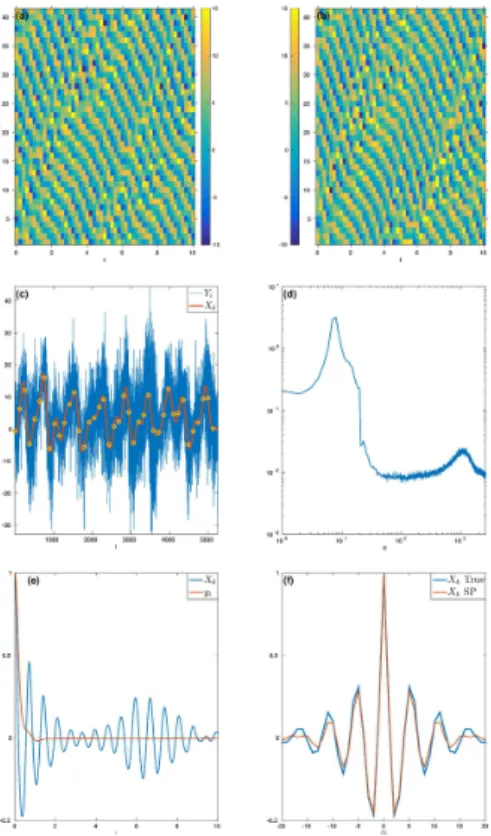
Some characteristics of the dynamics in regimes I and II are presented in Figs. 1 and 20

2, respectively. In regime I the large scale dynamics consist of a train of eight propa-gating and nonlinearly interacting “waves”, as seen in the time series of theXvariables in Fig. 1a. The large scale dynamics of the SP approximation are qualitatively simi-lar, as shown in Fig. 1b. The time-lagged autocorrelation function of theX_k variables (averaged overk) is shown in Fig. 1e, and displays an oscillatory structure associated 25

with the wave train. The initial decay of the time-lagged autocorrelation is approximated by an exponential of the form exp{−(λ+iω)t}with decorrelation time λ−1=0.84 and oscillation period 2π/ω=0.71; the resurgence of correlation between 6 and 8 time

(13)

NPGD

2, 513–536, 2015

Title Page

Tables Figures

◭ ◮

Back Close

Full Screen / Esc

Discussion

P

a

per

|

Discussion

P

a

per

|

Discussion

P

a

per

|

Discussion

P

a

per

|

units is associated with the time it takes a single wave to propagate once around the domain. The regularity of the wave train is also reflected in the space-lagged autocor-relation function for theXk variables shown in Fig. 1f, which is well approximated by

the SP dynamics. Figure 1c shows theY_i variables at an instant of time (blue), along with the large scale part (red; the projection onto the first 41 Fourier modes) and the 5

Xk variables (yellow circles). There is clearly strong small scale variability, but not so

strong that it completely obscures the large scale pattern, and the amplitude of the small scale variability varies over the domain. Figure 1d shows the time-averaged en-ergy spectrum|Yˆκ|2, where ˆYκ is the discrete Fourier coefficient ofYi with wavenumber

κ. There is a clear separation in amplitude between the large scale Fourier modes 10

(κ≤20) and the small scale modes, showing that the large scale energy is concen-trated near wavenumbers κ=7 and 8, while the small scale energy is more broadly distributed among Fourier modes. The broad distribution of small scale energy among Fourier modes is indicative of the strongly chaotic small scale dynamics, as is the rapid temporal decorrelation of the small scale variables yi shown in Fig. 1e. The

decorre-15

lation time of the small scale variablesy_i is estimated as 0.2 using the integral of the time-lagged autocorrelation function.

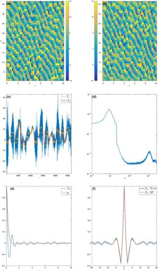
In regime II the large scale dynamics are more chaotic, though wave trains are still evident in the time series of X in Fig. 2a. The large scale dynamics of the SP ap-proximation are again qualitatively similar, as shown in Fig. 2b. The time-lagged au-20

tocorrelation function of theXk variables in Fig. 2e decays much more rapidly than in

regime I. The initial decay of the time-lagged autocorrelation is approximated by an ex-ponential of the form exp{−(λ+iω)t}with decorrelation timeλ−1=0.38 and oscillation period 2π/ω=0.95, and there is no resurgence of correlations at long lag times. The decreased regularity of the wave train is reflected in the space-lagged autocorrelation 25

function for theX_k variables shown in Fig. 2f, which is again well approximated by the SP dynamics. The snapshot of theYi variables in Fig. 2c shows a diminished level of

(14)

NPGD

2, 513–536, 2015

Title Page

Tables Figures

◭ ◮

Back Close

Full Screen / Esc

Discussion

P

a

per

|

Discussion

P

a

per

|

Discussion

P

a

per

|

Discussion

P

a

per

|

that the energy is more broadly distributed among large scale Fourier modes, though there is still a peak at wavenumberκ=8. The broad distribution of small scale energy among Fourier modes is again indicative of the strongly chaotic small scale dynamics, as is the rapid temporal decorrelation of the small scale variablesy_i shown in Fig. 2e. The decorrelation time of the small scale variablesy_i is estimated as 0.23 using the 5

integral of the time-lagged autocorrelation function.

TheY_i variables have a uniform time mean of 3.8 and 3.6 in regimes I and II, respec-tively, which is accurately reproduced by the SP approximation. TheX_k variables have variance 31 and 32 in regimes I and II, respectively, and their SP counterparts have slightly higher variances of 33 and 34. The small scale variablesy_i have climatological 10

variance of 70 in regime I and 29 in regime II, though Figs. 1c and 2c show that this variability is unevenly distributed over the physical domain at any given instant. Data assimilation experiments for both these regimes are described in the next section.

4 Assimilation experiments

In this section we describe data assimilation experiments in both regimes of the test 15

model of the foregoing section using the 3D-Var framework from Sect. 2 and the SP approximation described in the foregoing section. Observations are taken atP =MK

equispaced points with M=1, 2, and 4; specifically, observations are taken at ip=

1+pJ/Mforp=1,. . .,P. Observations are either linear, withvp=Yi_p+εp, or nonlinear,

withvp=(Yi_p+30)

2

/50+εp. In both cases the observation errorsεpare iid Gaussians

20

with zero mean and variance 0.1. Observations are assimilated every∆t time units. In

regime I we test∆t=0.2 and 0.6; for comparison the decorrelation times of the small

scale and large scale variables in this regime are 0.2 and 0.84. In regime II we test

∆t=0.2 and 0.4, which are close to the decorrelation times of the small scale and

large scale variables, respectively. 25

(15)

NPGD

2, 513–536, 2015

Title Page

Tables Figures

◭ ◮

Back Close

Full Screen / Esc

Discussion

P

a

per

|

Discussion

P

a

per

|

Discussion

P

a

per

|

Discussion

P

a

per

|

Specification of the background covariance matrix is a crucial aspect of any 3D-Var assimilation system. We consider the simplest possible estimate B=σ2I_K where I_K

is theK×K identity matrix and σ2 is a tunable parameter. Assimilation experiments are run over a range of σ2 and the optimal value is chosen based on RMS errors; the results are very weakly sensitive to σ2 as long as it is within a factor of 2 of the 5

diagnosed forecast error variance. Since our observing system includes at least one observation for everyX_k variable, it is less important to build a background covariance matrix with correlations between theX_k variables.

A single assimilation experiment consists of 1000 cycles, where the SP variables for the first forecast are initialized directly from the true model variables. Although the 10

assimilation system provides estimates of the small scale part of the true system at the location of the observations, this information is far from sufficient to provide an estimate of the full state Y of the true system. We view the 3D-Var assimilation as primarily aimed at estimating the large scale model variablesX_k, and error statistics are tracked only for the large scale variables. We track two performance metrics for the 15

large scale variables, the time averaged RMS error

RMS Error=kX−XSPk2 (27)

and the time averaged pattern correlation

Pattern Correlation= X

T

XSP

kXk2kXSPk2

(28)

both for the forecast and for the analysis. 20

As a point of comparison for the performance of the forecast in the assimilation experiments, we consider climatological values of RMS error and pattern correlation defined using the uniform climatological mean value ofXk as a prediction:Xk=3.8 in

regime I andX_k=3.6 in regime II. The climatological RMS error is simply the square root of the climatological variance: 5.6 in regime I and 5.7 in regime II. The climato-25

(16)

NPGD

2, 513–536, 2015

Title Page

Tables Figures

◭ ◮

Back Close

Full Screen / Esc

Discussion

P

a

per

|

Discussion

P

a

per

|

Discussion

P

a

per

|

Discussion

P

a

per

|

uniform climatological mean value: 0.57 in regime I and 0.53 in regime II. If the forecast has larger RMS error or smaller pattern correlation than the climatological values then the forecast is of very limited utility.

As a point of comparison for the performance of the analysis estimate in the assimi-lation experiments we take a “smoothed observation” estimate that is obtained by pro-5

jecting the observations onto the largestK Fourier modes. For example, whenM=1 there are K observations and the “smoothed observation” estimate of the X_k vari-ables is simplyX_k≈v_pfor the linear case andX_k≈q50v_p−30 for the nonlinear case. The RMS errors in the smoothed observation estimate are tracked over the course of each assimilation experiment, rather than computing climatological values. The 3D-Var 10

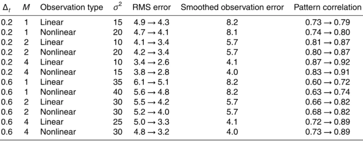
should at a minimum perform better than the smoothed observations. The results for both regimes are presented in Tables 1 and 2 in the format Forecast→Analysis. In all cases the errors decrease asM increases, and the analysis significantly improves over the forecast.

The large scale dynamics are more predictable in regime I than in regime II, but the 15

small scale variance is larger as well, making it harder to obtain an accurate estimate of the large scales. With a short observation time∆t=0.2, the forecast and analysis for

linear and nonlinear observations both have RMS errors smaller than both the climato-logical error of 5.6 and the error in the smoothed observation estimate. The nonlinear observations generate slightly more accurate results than the linear observations when 20

M=1, and the linear observations generate slightly more accurate results for M=4, but overall the results are similar. With a longer observation time∆t=0.6 the results

are, naturally, less accurate. In every case the analysis is more accurate than both the climatological error and the smoothed observations, but the forecasts are more accu-rate than the climatological mean only withM=4. WithM=1 and 2, the RMS forecast 25

errors are worse than the climatological error, but the forecast pattern correlations are still a bit better than the climatological pattern correlation. As with the shorter observa-tion time, the results are more accurate with the nonlinear observaobserva-tions.

(17)

NPGD

2, 513–536, 2015

Title Page

Tables Figures

◭ ◮

Back Close

Full Screen / Esc

Discussion

P

a

per

|

Discussion

P

a

per

|

Discussion

P

a

per

|

Discussion

P

a

per

|

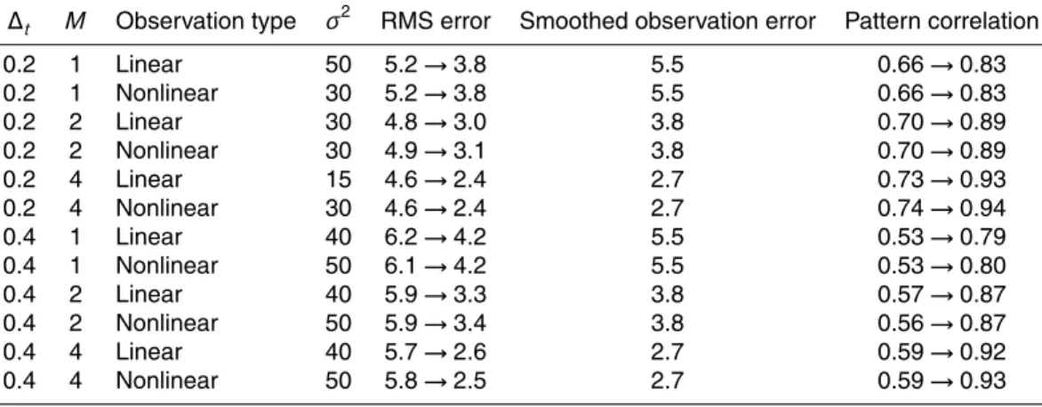
In regime II the results with the linear and nonlinear observations are very similar in all cases. With a short observation time ∆t=0.2, the forecast is always more

ac-curate than the climatological mean, and the analysis is always more acac-curate than the smoothed observations. With a longer observation time∆t=0.4 the forecasts are

no more accurate than climatology, but the analysis is still more accurate than the 5

smoothed observations, though atM=4 the analysis is only slightly more accurate.

5 Conclusions

Superparameterization (SP) is a multiscale computational approach that has been suc-cessfully applied to modeling atmospheric dynamics, and that shows promise for more general applications (Tao et al., 2009; Randall et al., 2013; Majda and Grooms, 2014). 10

Grooms et al. (2014) have developed an ensemble Kalman filter framework for use with SP, but the standard approach to SP in global atmosphere and climate models, where small scale nonlinear dynamics are simulated on an array of periodic domains embed-ded in the computational grid of a large scale model, is too computationally demanding for use in an ensemble framework. We here develop a 3D-Var variational data assim-15

ilation framework for SP that builds on and modifies the framework of GLM14. The main update to the GLM14 framework, in addition to using a variational as opposed to ensemble Kalman filter setting, is that small scale estimates are computed at locations where observations are taken, rather than at every point of the large scale model’s computational grid.

20

The data assimilation framework is demonstrated in a new system of ordinary dif-ferential equations based on the two-scale Lorenz-’96 model (Lorenz, 1996, 2006). Unlike the two-scale Lorenz-’96 model the new model has only one set of variables,Y_i, and these variables have large and small scale parts. An SP approximation to the new system is developed, which is perhaps the simplest idealized model of SP. The new 25

(18)

NPGD

2, 513–536, 2015

Title Page

Tables Figures

◭ ◮

Back Close

Full Screen / Esc

Discussion

P

a

per

|

Discussion

P

a

per

|

Discussion

P

a

per

|

Discussion

P

a

per

|

a weakly chaotic wave train, with relatively strong small scale variability superposed. In regime II the large scale dynamics are more strongly chaotic, and there is less small scale variability. In both regimes the data assimilation performs as expected, with in-creased accuracy as the number of observations increases.

Our work lays a foundation for 3D-Var data assimilation with existing SP models. 5

The main difficulty in using the framework with an SP atmosphere or climate model is in specifying an appropriate background covariance matrix for the large scale model, but this difficulty should not be insurmountable given the extensive use of the 3D-Var approach in atmosphere and ocean data assimilation (e.g. Kalnay, 2002; Kleist et al., 2009). In addition, the new framework removes one of the difficulties associated with 10

development of a 3D-Var framework for large scale models: the small scale simulations in the multiscale SP computation provide direct information on the small scale statistics, obviating, or at least simplifying, the need to develop models of representation error.

Author contributions. I. Grooms designed the research, I. Grooms and Y. Lee carried out the experiments, and I. Grooms prepared the manuscript.

15

Acknowledgements. The authors acknowledge funding from the United States Office of Naval Research MURI grant N00014-12-1-0912. The authors thank A. J. Majda for suggesting the addition of a second regime (regime II).

References

Abramov, R. V.: Suppression of chaos at slow variables by rapidly mixing fast dynamics through

20

linear energy-preserving coupling, Commun. Math. Sci., 10, 595–624, 2012. 524

Grabowski, W.: An improved framework for superparameterization, J. Atmos. Sci., 61, 1940– 1952, 2004. 523

Grabowski, W. and Smolarkiewicz, P.: CRCP: a Cloud Resolving Convection Parameterization for modeling the tropical convecting atmosphere, Physica D, 133, 171–178, 1999. 514

25

Grooms, I. and Majda, A. J.: Efficient stochastic superparameterization for geophysical turbu-lence, P. Natl. Acad. Sci. USA, 110, 4464–4469, doi:10.1073/pnas.1302548110, 2013. 515

(19)

NPGD

2, 513–536, 2015

Title Page

Tables Figures

◭ ◮

Back Close

Full Screen / Esc

Discussion

P

a

per

|

Discussion

P

a

per

|

Discussion

P

a

per

|

Discussion

P

a

per

|

Grooms, I. and Majda, A. J.: Stochastic superparameterization in a one-dimensional model for wave turbulence, Commun. Math. Sci., 12, 509–525, 2014a. 515

Grooms, I. and Majda, A. J.: Stochastic superparameterization in quasigeostrophic turbu-lence, J. Comput. Phys., 271, 78–98, 2014b. 515

Grooms, I., Lee, Y., and Majda, A. J.: Ensemble Kalman filters for dynamical systems with

un-5

resolved turbulence, J. Comput. Phys., 273, 435–452, doi:10.1016/j.jcp.2014.05.037, 2014. 515, 529

Grooms, I., Majda, A. J., and Smith, K. S.: Stochastic superparameterization in a quasi-geostrophic model of the Antarctic Circumpolar Current, Ocean Model., 85, 1–15, 2015. 515

10

Harlim, J. and Majda, A. J.: Test models for filtering with superparameterization, Multiscale Model. Sim., 11, 282–308, 2013. 521

Kalnay, E.: Atmospheric Modeling, Data Assimilation, and Predictability, Cambridge University Press, 2002. 530

Khairoutdinov, M. and Randall, D.: A cloud resolving model as a cloud parameterization in

15

the NCAR Community Climate System Model: preliminary results, Geophys. Res. Lett., 28, 3617–3620, doi:10.1029/2001GL013552, 2001. 514

Khairoutdinov, M., Randall, D., and DeMott, C.: Simulations of the atmospheric general circu-lation using a cloud-resolving model as a superparameterization of physical processes, J. Atmos. Sci., 62, 2136–2154, doi:10.1175/JAS3453.1, 2005. 515

20

Kleist, D. T., Parrish, D. F., Derber, J. C., Treadon, R., Wu, W.-S., and Lord, S.: Introduction of the GSI into the NCEP global data assimilation system, Weather Forecast., 24, 1691–1705, 2009. 530

Lorenz, E.: Predictability: a problem partly solved, in: Proceedings of Seminar on Predicability, vol. 1, ECMWF, Reading, UK, 1–18, 1996. 516, 521, 529

25

Lorenz, E.: Predictability: a problem partly solved, in: Predictability of Weather and Climate, edited by: Palmer, T. and Hagedorn, R., Cambridge University Press, 40–58, 2006. 516, 521, 529

Majda, A. J. and Grooms, I.: New perspectives on superparameterization for geophysical tur-bulence, J. Comput. Phys., 271, 60–77, doi:10.1016/j.jcp.2013.09.014, 2014. 515, 529

30

(20)

NPGD

2, 513–536, 2015

Title Page

Tables Figures

◭ ◮

Back Close

Full Screen / Esc

Discussion

P

a

per

|

Discussion

P

a

per

|

Discussion

P

a

per

|

Discussion

P

a

per

|

Randall, D., Khairoutdinov, M., Arakawa, A., and Grabowski, W.: Breaking the cloud parame-terization deadlock, B. Am. Meteorol. Soc., 84, 1547–1564, 2003. 514

Randall, D., Branson, M., Wang, M., Ghan, S., Craig, C., Gettelman, A., and Edwards, J.: A community atmosphere model with superparameterized clouds, EOS T. Am. Geophys. Un., 94, 221–228, 2013. 514, 529

5

Talagrand, O.: Variational assimilation, in: Data Assimilation Making Sense of Observations, edited by: Lahoz, W., Khattatov, B., and Menard, R., Springer, Berlin, Heidelberg, 41–67, doi:10.1007/978-3-540-74703-1_3, 2010. 519

Tao, W.-K., Anderson, D., Chern, J., Entin, J., Hou, A., Houser, P., Kakar, R., Lang, S., Lau, W., Peters-Lidard, C., Li, X., Matsui, T., Rienecker, M., Schoeberl, M. R., Shen, B.-W., Shi, J. J.,

10

and Zeng, X.: The Goddard multi-scale modeling system with unified physics, Ann. Geophys., 27, 3055–3064, doi:10.5194/angeo-27-3055-2009, 2009. 514, 529

Wilks, D. S.: “Superparameterization” and statistical emulation in the Lorenz ’96 system, Q. J. Roy. Meteorol. Soc., 138, 1379–1387, doi:10.1002/qj.1866, 2012. 521

(21)

NPGD

2, 513–536, 2015

Title Page

Tables Figures

◭ ◮

Back Close

Full Screen / Esc

Discussion

P

a

per

|

Discussion

P

a

per

|

Discussion

P

a

per

|

Discussion

P

a

per

|

Table 1.Results of the assimilation experiments for regime I. There areP =MK equispaced observations, assimilated at time intervals of∆t, and σ

2

is the amplitude of the background covariance matrix. For comparison, the climatological RMS error and pattern correlation are 5.6 and 0.57.

∆t M Observation type σ2 RMS error Smoothed observation error Pattern correlation

0.2 1 Linear 15 4.9→4.3 8.2 0.73→0.79

0.2 1 Nonlinear 20 4.7→4.1 8.1 0.74→0.80

0.2 2 Linear 10 4.1→3.4 5.7 0.81→0.87

0.2 2 Nonlinear 20 4.2→3.4 5.7 0.80→0.87

0.2 4 Linear 10 3.4→2.6 4.1 0.87→0.92

0.2 4 Nonlinear 15 3.8→2.8 4.0 0.83→0.91

0.6 1 Linear 35 6.1→5.1 8.2 0.60→0.72

0.6 1 Nonlinear 40 5.6→4.8 8.2 0.63→0.74

0.6 2 Linear 30 5.5→4.2 5.7 0.66→0.82

0.6 2 Nonlinear 30 5.2→4.0 5.7 0.68→0.82

0.6 4 Linear 25 5.0→3.3 4.1 0.72→0.89

(22)

NPGD

2, 513–536, 2015

Title Page

Tables Figures

◭ ◮

Back Close

Full Screen / Esc

Discussion

P

a

per

|

Discussion

P

a

per

|

Discussion

P

a

per

|

Discussion

P

a

per

|

Table 2.Results of the assimilation experiments for regime II. There areP =MK equispaced observations, assimilated at time intervals of∆t, and σ

2

is the amplitude of the background covariance matrix. For comparison, the climatological RMS error and pattern correlation are 5.7 and 0.53.

∆t M Observation type σ2 RMS error Smoothed observation error Pattern correlation

0.2 1 Linear 50 5.2→3.8 5.5 0.66→0.83

0.2 1 Nonlinear 30 5.2→3.8 5.5 0.66→0.83

0.2 2 Linear 30 4.8→3.0 3.8 0.70→0.89

0.2 2 Nonlinear 30 4.9→3.1 3.8 0.70→0.89

0.2 4 Linear 15 4.6→2.4 2.7 0.73→0.93

0.2 4 Nonlinear 30 4.6→2.4 2.7 0.74→0.94

0.4 1 Linear 40 6.2→4.2 5.5 0.53→0.79

0.4 1 Nonlinear 50 6.1→4.2 5.5 0.53→0.80

0.4 2 Linear 40 5.9→3.3 3.8 0.57→0.87

0.4 2 Nonlinear 50 5.9→3.4 3.8 0.56→0.87

0.4 4 Linear 40 5.7→2.6 2.7 0.59→0.92

0.4 4 Nonlinear 50 5.8→2.5 2.7 0.59→0.93

(23)

NPGD

2, 513–536, 2015

Title Page

Tables Figures

◭ ◮

Back Close

Full Screen / Esc

Discussion

P

a

per

|

Discussion

P

a

per

|

Discussion

P

a

per

|

Discussion

P

a

per

|

(24)

NPGD

2, 513–536, 2015

Title Page

Tables Figures

◭ ◮

Back Close

Full Screen / Esc

Discussion

P

a

per

|

Discussion

P

a

per

|

Discussion

P

a

per

|

Discussion

P

a

per

|

Figure 2.Climatological statistics in regime II. Panels are the same as Fig. 1.