FUNDAC
¸ ˜
AO GETULIO VARGAS
ESCOLA DE P ´
OS-GRADUAC
¸ ˜
AO EM
ECONOMIA
Francisco Luis Lima Filho
Environmental Regulation, Technology Adoption and
Structural Transformation: Evidence from Brazilian
Sugarcane Industry
Rio de Janeiro
Francisco Luis Lima Filho
Environmental Regulation, Technology Adoption and
Structural Transformation: Evidence from Brazilian
Sugarcane Industry
Disserta¸c˜ao submetida a Escola de
P´os-Gradua¸c˜ao em Economia como requisito
par-cial para a obten¸c˜ao do grau de Mestre em
Economia.
´
Area de Concentra¸c˜ao: Microeconomia Emp´ırica
Orientador: Francisco Costa
Rio de Janeiro
Ficha catalográfica elaborada pela Biblioteca Mario Henrique Simonsen/FGV
Lima Filho, Francisco Luis
Environmental regulation, technology adoption and structural transformation: evidence from Brazilian sugarcane industry / Francisco Luis Lima Filho. – 2015. 38 f.
Dissertação (mestrado) - Fundação Getulio Vargas, Escola de Pós-Graduação em Economia.
Orientador: Francisco Costa. Inclui bibliografia.
Abstract
We estimate the effects of the adoption of mechanized agriculture led by a new en-vironmental regulation on structural change of local labor markets within a large emerging country, Brazil. In 2002, the state of S˜ao Paulo passed a law outlying the timeline to end sugarcane pre-harvest burning in the state. The environmental law led to the fast adoption of mechanized harvest. We investigate if the labor intensity of sugarcane production decreases; and, if so, if it leads to structural changes in the labor market. We use satellite data containing the type of sugarcane harvest-ing – manual or mechanic harvest – paired with official labor market data.We find suggestive evidence that mechanization of the field led to an increase in utilization of formal workers and a reduction in formal labor intensity in the sugarcane sec-tor. This is partially compensated by an increase in the share of workers in other agricultural crops and in the construction and services sector. Although we find a reduction in employment in the manufacturing sector, the demand generated by the new agro-industries affected positively the all sectors via an increase in workers’ wage.
Contents
1 Introduction 8
2 Background 12
3 Empirical Strategy and Data 14
3.1 Data . . . 14
3.2 Empirical Strategy . . . 16
3.3 Main Regression . . . 17
3.4 Instrumental Variable . . . 18
4 Empirical Results 20
5 Robustness Check 23
6 Conclusion 24
List of Figures
1 Clean Harvesting vs Slope first moment . . . 28
2 Clean Adoption Index vs Slope first moment . . . 28
3 Clean Adoption Index vs Slope second moment . . . 29
4 Planted Area Expansion vs Slope first moment . . . 29
5 Lowess Planted Area Expansion vs Slope first moment . . . 30
List of Tables
1 Sugarcane Production (thousands ton) . . . 312 Timeline . . . 31
3 Mechanical Harvesting Evolution (%) . . . 31
4 Employees in the Sugarcane Industry (2007) . . . 32
5 Descriptive Statistics: Independent Variables . . . 32
6 Descriptive Statistics: Dependent Variables . . . 33
7 First Stage . . . 34
8 OLS and 2SLS . . . 35
9 Municipality Robustness Check: First Stage . . . 36
10 Municipality Robustness Check: OLS and 2SLS . . . 37
1
Introduction
The main focus of environmental regulation is to correct for externalities and other
market failures. Very often, in order to comply with new environmental goals, the
produc-tive sector needs to adopt new and cleaner technologies. In particular in agriculture,
tech-nological changes may trigger structural transformation as it changes the factor-content
of production in the field and/or generates demand for services and manufacturing goods.
Matsuyama (1992) and Bustos et al. (2013) argue that the positive impacts of
agricul-tural productivity on industrialization occur only in closed economies (e.g., productivity
growth in agriculture can release labor or generate demand for manufacturing goods),
while in open economies the impacts are indeterminate because comparative advantage
in agriculture can reduce industrial growth. What happens is that the agricultural sector
will employ more workers because of the increase in productivity, what reduces
manufac-turing sector and its benefits from external scale economies.
This paper estimates the causal effects of the adoption of mechanized agriculture led
by a new environmental regulation on structural change of local labor markets within
a large emerging country, Brazil. Our object is an environmental law aimed at ending
sugarcane pre-harvest burning, which promoted the adoption of mechanical sugarcane
harvesting. We investigate two underlying questions: is harvest mechanization a labor
saving technical change – i.e., does the labor intensity of sugarcane production decrease?;
and, if so, does harvest mechanization lead to structural changes in the local labor market?
Sugarcane is one of the main crops in Brazil and world’s largest crop by production
quantity (Walter et al., 2014). In 2012, FAO estimates that sugarcane was cultivated on
about 26.0 million hectares, in more than 90 countries, with a worldwide harvest of 1.83
billion tons. Sugarcane can be harvested using two different technologies: the traditional
one, by hand with necessary pre-harvest field burning; or mechanically, mainly without
pre-harvest burning.1 Sugarcane straw burning is responsible for a great amount of
pollutant gases in atmosphere (Macedo et al., 2008) which cause respiratory diseases
in the local population (Can¸cado et al., 2006; Dominici et al., 2014; Rangel and Vogl,
2015). Many other countries already implemented environmental regulation to correct
this externality that arises from the productivity side of the economy (e.g., Greenstone
1
(2002); Greenstone and Hanna (2014); Barreca et al. (2014).
In Brazil, the state of So Paulo the richest and largest producer state passed a law
in 2002 outlying a timeline to end sugarcane pre-harvest burning on large properties by
2021. In 2007, the Cooperation Protocol was sealed between So Paulo state and the
Or-ganization of Sugarcane Producers (ORPLANA). The phase out process was accelerated
with the deadline being shortened to 2014, and with the creation of an agro-environmental
certificate for unburnt sugarcane. The environmental law and the new protocol led to
the fast adoption of mechanized harvest. In 2008 49.1% of the harvest area in So Paulo
was without pre-harvest burning, while in 2012 this number increased to 72.6%, we also
see a increase in total harvest area in this period.
The expansion of mechanical harvest can affect labor demand in the sugarcane sector
through two channels. First, less workers are needed to harvest the same planted area.
Second, this changes the work relations with more formal workers being employed and
less temporary workers. Given the size of this sector in many localities, a technological
change in this sector could have impacts on the remaining sectors of the economy.
We use two main datasets to investigate this relation: remote sensing data with
sug-arcane production by harvest type (CANASAT/INPE), and matched employer-employee
dataset with the universe of formal workers in Brazil (RAIS/MTE). We use the
satel-lite data to create our measure for the evolution of adoption of mechanization in
sug-arcane production in different microregions. We construct a clean adoption index that
defines the intensity of mechanization in sugarcane as the fraction of land (pixels) without
pre-harvesting burning out of the total number of land (pixels) with sugarcane harvest,
relative to the baseline mechanization intensity in 2006, which is a way to observe
mecha-nization in sugarcane production. We create a balanced panel of microregions, from 2006
to 2012.
In order to unveil the causal relation between the adoption of mechanized harvest
technology and labor market outcomes, we use an instrumental variable strategy. We
use the first two moments of land slope as an instrument for harvest mechanization, this
is georeferenced topographical data (TOPODATA). The intuition for this instrument is
that it is more costly to adopt mechanized harvest in steeper plots of land. We find a
negative relation between the land slope and, both, the expansion of mechanization and
the evolution of labor market outcome directly, but only indirectly via the adoption of
technologies in the field.
Using the registers of all formally employed workers aggregated at the sector-local
la-bor market level, we find that the adoption of clean harvesting reduces, not statistically,
the formal labor intensity per plot of land. We find weak evidence that the new
tech-nology increases the number of formal permanent jobs in the sugarcane sector, however,
we see a reduction in the employment share of this sector at the microregion-year level.
We find that this reduction may have been compensated by an increase in the number of
workers in the “construction and services” and agriculture sectors and a decrease in the
manufacturing sector, all not statistically significant. Interestingly, we find economically
meaningful but not statistically significant increase in the total wages at all sectors and
in the average worker wage. We interpret these results as suggestive evidence that
mech-anization of the field leads to an increase in utilization of formal workers as well as with
an increase in their productivity in a manner that it reduces formal labor intensity and
increases wages in the sugarcane sector. Although this may represent less labor supply
for industries, the demand generated by the new agro-industries affects positively workers
via wages in all other sectors.
Several previous studies try to understand what the determinants of technology
adop-tion in non-developed economies (Esther Duflo and Robinson, 2006; Conley and Udry,
2010; Bandiera and Rasul, 2002). Esther Duflo and Robinson (2006) tries to measure
the returns to fertilizer use through a field experiment with farmers in Kenya. Miguel
and Kremer (2004) study of the adoption of wormicide pills among school-age children
in Kenya, for example, found that deworming improved health and school participation
in both treatment schools and neighboring schools. Foster and Rosenzweig (2010) argues
that the net gains, inclusive the new costs, are important determinants of a new
tech-nology adoption. When considering profit-maximizing entities, Foster and Rosenzweig
(2010) says that is clear that technology profitability is the key for technology adoption,
agents decide to use a technology based on the gain in welfare, which cannot be directly
measured, in the case of medical technologies (e.g., bed nets, water purifiers, curative
pills) adoption will depend on how health is valued. In our case, environmental
regu-lation wants reduces pollutant gases, what may reduce respiratory diseases caused by
labor markets.
This paper contributes to the literature on the consequences of technology adoption on
local development by showing how sugarcane harvest mechanization affects workers’ labor
market outcomes (Berman et al., 1998; Beaudry et al., 2006). Also, to the literature of
environmental regulation consequences on local labor markets (Kahn and Mansur, 2013;
Deschenes, 2010). We see evidence that sugarcane mechanization increases wages at
manufacturing, construction and services, and also agricultural sectors.
At last, we also contribute to the literature on structural transformation. Matsuyama
(1992) shows that for small open economies facing perfectly elastic demand for
agricul-tural and manufacturing goods the demand and supply channels on labor markets are
no longer operative. His model – which has only one type of production factor, labor –
predicts that a Hicks-neutral increase in agricultural productivity reduces the industrial
sector by reallocating labor towards agriculture. Bustos et al. (2013), however, differ
from Matsuyama (1992) by using two production factors, land and labor. In this case,
technical change can be factor-biased. When technical change in agriculture is strongly
labor saving, an increase in agricultural productivity leads to manufacturing growth as
it increases residual labor supply even in open economies. Bustos et al. (2013) provides
direct empirical evidence on the effects of technical change in agriculture on the industrial
sector by studying the effects of the adoption of genetically engineered soybean seeds – a
labor saving technology change –, and the adoption of second-harvest maize – a labor
de-manding technology change – in Brazil. Their findings corroborate the model predictions.
Our paper provides suggestive evidence that the adoption of a labor saving technology,
which weakly reduce the labor-land ratio, reduced the size of the manufacturing sector.
The remaining of this work is organized as follows: section 2 gives background
in-formation on sugarcane harvesting and labor market in Brazil; section 3 describes the
data and our empirical strategy; section 4 presents our empirical results; section 5 shows
a robustness check; and, section 6 concludes this work pointing the direction of this
2
Background
In this section we briefly discuss the sugarcane industry background in Brazil and in
So Paulo state, the largest producer in the country. Two main aspects are discussed:
harvesting and labor market.
Sugarcane is one of the main crops in Brazil and world’s largest crop by production
quantity (Walter et al., 2014). In 2012, FAO estimates about 26.0 million hectares of
cultivated area, in more than 90 countries, with a worldwide harvest about 1.83 billion
tons. Brazil being the top producer responsible for more then a quarter of worldwide
production. According to UNICA (Sugarcane Industry Union), So Paulo state contributes
with more then a half of Brazilian production as in Table 1. Sugarcane is a semi-perennial
crop that, in So Paulo State, reaches its maximum vegetative development in April.
Its planting can be done at two moments: at SeptemberOctober, when twelve-month
sugarcane is planted; or at FebruaryMarch, when eighteen-month sugarcane is planted.
And the sugarcane harvesting happens between April and December.
There are two harvesting technologies: the traditional one, by hand with pre-harvest
field burning; and mechanically, without burning. In hand harvesting, field burning
is necessary because of ergonomic restrictions, to clean the area from other weeds and
to chase away any dangerous animals. However, mechanical harvesting can be made
without burning, keeping leaves and straws intact, what is called called green or clean
harvesting. Leaves and straws can be used for energy production or as vegetable coverage
for conventional or organic agriculture. The sugarcane straw burning produces a negative
externality and is responsible for a great amount of pollutant gases in atmosphere (Macedo
et al., 2008) which cause respiratory diseases in the local population (Can¸cado et al., 2006;
Dominici et al., 2014; Rangel and Vogl, 2015). Other environmental problems related to
sugarcane straw burning were soil and groundwater contamination (Brasil, 2009).
With the goal of mitigating climate change problems and respiratory diseases, in 2002,
the state of So Paulo passed a law outlying the timeline to end sugarcane pre-harvest
burning. There was two calendars with the targets to adopt mechanical harvest according
to the slope of the land: mechanizable areas, properties bigger than 150 hectares and with
slope greater or equal to 12%; and non-mechanizable areas, properties smaller than 150
hectares or with slope greater than 12% or with soil structures impossible to mechanize.
In 2007, the Cooperation Protocol was sealed between So Paulo state and the
Orga-nization of Sugarcane Producers (ORPLANA). The phase out process was accelerated
with the deadline being shortened to 2014 for properties with slope less or equal 12%,
or to 2021 for properties with slope greater than 12%, and with the creation of an
agro-environmental certificate for unburnt sugarcane. The Protocol also anticipated the
re-duction of burning practices from 50% to 70% in 2010 for properties with slope less or
equal 12%, and from 10% to 30% in 2010 for properties with slope greater than 12%.
For this protocol, there is no differentiation between mechanizable or non-mechanizable
areas, only in slope level. 2
Novaes et al. (2007) point out three elements about the adoption of mechanized
tech-nology. First, the prohibition of the pre-harvest burning would reduce directly the hand
harvesting productivity. Second, there are natural conditions for machinery
introduc-tion, it is easier to do mechanic harvesting in more flat terrain. Third, the increase in
labor productivity and the low wages in hand harvesting are an obstacle to mechanical
harvesting.
Table 3 shows the evolution on mechanical harvest in the Center-South region, where
So Paulo state is located. Since mechanical harvest can be made with or without
pre-harvest burning we make this distinction in the table. We can see that around 80% of
the mechanical harvesting is unburnt. With this table we see a reversal in the type of
sugarcane harvesting, in 2006 hand harvesting comprehended 63.3% while in 2012 this
number reduced to 14.9%. Also we see that in 2006, around 30% of mechanical harvesting
used pre-harvesting burning while in 2012 this number reduced to 15%.
The sugarcane ethanol sector has a bad record in labor relations and environmental
rules.3. In 2007, there were around 498 thousand formal employees in the sugarcane crop
activity, 54% in the state of So Paulo. In the sugarcane crop, especially in hand
harvest-ing, the most part are of unskilled and temporary jobs, with different levels according to
seasons. Table 4 shows that aggregating the whole sugarcane industry in 2007, we had
2
Braunbeck and Magalh˜aes (2010) discuss some issues that might be considered before mechanizing harvest. One of them is the maximal slope that is able to mechanizing. Theoretically it should be 46% but because of ground irregularities and other driving problems the critical slope is 12%. It should lead to the end of sugarcane production in steep areas. However, with advances in the off-road vehicle engineering such as four wheel drive, harvesters can be used in terrains with slopes greater than 12% around 15%-18%.
3
a total of 1.26 million formal workers, 520 thousand in So Paulo, with 270 thousands
working directly in sugarcane crop. 91% of the formal workers were under 50 years old,
52% had 4 years of study or less and 7% were illiterate. However, in the past few years,
with the expansion of mechanical harvesting, the sugarcane industry started recruiting
more skilled workers, substituting the hand worker for machine operators and other
occu-pations (e.g., engineers and mechanics). According to some estimates from the industry
(SGPR, 2009), one harvest machine can substitute eighty hand workers.
In 2009, was signed the National Agreement to Improve Sugarcane Working
Condi-tions between UNICA, by the Federal Government and the National Confederation of
Agricultural Workers (CONTAG). This Agreement was about improving better labor
practices and to promoting the reintegration of workers unemployed by the advance in
mechanized harvesting.
3
Empirical Strategy and Data
This section is divided in two subsections, first we describe the three main data
sources used in this paper and briefly present how we treated the data. Then, we describe
our empirical strategy, where we first discuss some problems that could appear from a
Ordinary Least Squares (OLS) approach and then present our Two Stages Least Squares
(2SLS).
3.1
Data
We use three main data sources: formal register of employees (the Annual Report
of Social Information - RAIS); spatial data of sugarcane harvesting type
(CANASAT-INPE); and geomorphometric data in Brazil (TOPODATA).
RAIS consists in a national database that processes formal labor market statistics,
containing all information across years from all formal workers in Brazil. Every
com-mercial establishment must report to the ministry of Employment and Labor (MTE),
through RAIS, information about all employees. The main variables we use from RAIS
are: number of workers (permanent and temporary), total wage (the sum of all monthly
wages at microregion and also at municipality) and average worker wage (the reason of
RAIS, we also generate some variables: employment share (the fraction of one sector
in the total amount of formal workers), and formal labor intensity (number of workers
per harvested area). Although we have the individual level data, at this preliminary
stage we aggregate all variables at the microregion level to investigate the impact of the
mechanized harvest adoption in the local labor market. We use CNAE 2.0 to separate
the market in four sectors: sugarcane (code 113), agriculture (codes from 1 to 999 and
different from 113), industry (codes from 1000 to 3390), and construction and services
(codes from 4100 to 9799).
INPE has two different data base: Planted Area; and
CANASAT-Harvest. CANASAT-Planted Area annually monitors sugarcane planted area in different
classes and regions between 2003/04 and 2013/14. CANASAT-Harvest monitors
sug-arcane harvest of So Paulo state from 2006/07 to 2012/13, distinguishing two types of
harvesting: with or without pre-harvest burning (Rudorff et al., 2010; Adami et al.,
2012). CANASAT-Harvest uses visual interpretation technique of remote sensing
im-ages, obtained between April and December in each crop year, to identify and map the
two types of sugarcane harvest practices. Most of the sugarcane harvesting is performed
during the dry season, when it is relatively favorable to acquire cloud free images.
Iden-tification of harvest type is based on the reflectance difference between green harvested
and pre-harvest burned fields (Aguiar et al., 2011).
TOPODATA project offers the Digital Elevation Model (MDE) and its derivations
at national level. MDE is a computational mathematic representation of a spatial
phe-nomenon. The original data is from the Shuttle Radar Topography Mission (SRTM),
which is an international research effort that obtained digital elevation models on a
near-global scale to generate the most complete high-resolution digital topographic database
of Earth. The resolution of the raw data is one arcsecond, but this has only been released
over United States territory, for Brazil the resolution is 3 arcseconds. The resolution used
in this work is thirty arcsecond the same as half arcminute.
We aggregate the remote sensing data at half arcminute level, also. From CANASAT,
we have the distribution of harvesting and planted area across So Paulo state. Using this
information we add up at municipality level and then at microregion level, our variable is
the number of pixels of each harvesting type or the number of pixels with planted area.
we have the distribution of slope across So Paulo state. Using this distribution we
aggre-gate at municipality level and calculate some moments and after at microregion level, for
this work we use the first and the second.
We create a balanced panel of microregions from 2006 to 2012, with 44 microregions,
where we observe at least one type of sugarcane harvesting all years. Finally, in order to
perform some robustness checks we disaggregate our variables at the municipality level.
We then have 408 municipalities with some sugarcane harvesting from 2006 to 2012.
3.2
Empirical Strategy
We need to measure how much of the sugarcane harvesting is clean, in order to capture
mechanization, and we observe this in data. Thus, our empirical strategy begins with a
construction of a clean technology index. This index consists in the proportion of land
plots with clean harvesting in the microregion. Such as the formula below:
CleanIndexjt ≡
Cleanjt
HarvestedAreajt
(1)
WhereCleanjt represents the number of pixels with green harvesting, andHarvestedAreajt
the total number of pixels with harvesting, at microregion j and year t. Notice that this
clean technology index is bounded between 0 and 1, so microregions that do all the
harvest using green technology has 1 and microregions using only pre-harvest burning
technology get 0. The interpretation of these numbers are: microregions with 1 use only
mechanized harvest, but this does not mean that microregions with a 0 use only hand
harvest because we can do pre-harvest burning and still use mechanical harvesting, as
discussed in background section.
We define our clean technology adoption index:
CleanAdoptionIndexjt ≡∆CleanIndexjt =CleanIndexjt−CleanIndexj,2006 (2)
Where CleanIndexj,2006 is the share of the total number of pixels with harvesting with
3.3
Main Regression
Our variables of interest are labor market outcomes like labor intensity in the
sug-arcane industry, employment share, number of total employees logarithm, number of
permanent employees logarithm, total wage logarithm, average worker wage logarithm.
We evaluate the evolution of these variables relative to 2006 (∆Yijt ≡ Yijt Yij2006), in
order to make them consistent with our clean adoption index. Variables are indexed by
productivity (cnae) sector (i), microregion (j), and year (t).
Our main regression equation is:
∆Yijt =βCleanAdoptionIndexjt+γXjt+νijt (3)
Where Xjt are time and microregions controls, like year dummy variables, and total
harvesting and clean harvesting in 2006.
This OLS specification that may present some identification problems. There may
have some endogenous relation between labor market development and adoption of new
mechanized technology in the field, so causal relations are not clear. For example, consider
a shock in labor market increasing wages at a level that producers prefer paying fixed
costs of mechanical harvest and employing few workers than making only hand harvest
employing more workers. Now consider the case of a positive shock to investments in the
local economy, for example government subsidies. In this scenario technology adoption
may be cheaper by itself and labor market outcomes would improve anyway.
This analysis can be extended to the whole microregion economy, using a general
equilibrium scope. Consider a shock in machinery prices, like a reduction of import
tariffs. This would impact positively in clean harvesting and in industrialization – and
in others sectors too. What would be the final effect in labor market? One hypothetic
scenario could be a labor saving investment in manufacturing sector increasing labor offer
in that microregion, that could make more profitable invest in hand harvesting rather than
in clean harvesting. Now think the other direction, increase of clean harvesting making
attractive for the manufacturing firms to employ more workers rather than buying more
productive machines.
We do our analysis at microregion level because municipalities are commonly
In order to see the difference of labor market changes between microregion and
munici-pality level we redo all estimations at municimunici-pality level as a robustness check.
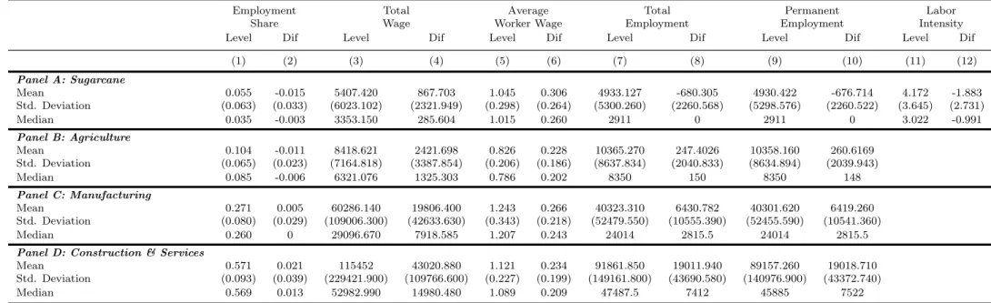
Tables 5 and 6 report summary statistics. Table 5 presents summary statistics of
our independent variables, controls, clean adoption index and instruments. In table 6
we present summary statistics of our dependent variables in level and in difference from
2006, mean, standard deviation, and median.
3.4
Instrumental Variable
In order to avoid endogeneity and to find some causality we look for instrumental
variables. Our candidate is the first and second moments of land slope at the microregion
level. The first moment is a strong candidate because the law is different according to
the slope of the terrain and also because of the discussion about technical problems and
solutions to mechanical harvesting in steep terrain. What we have in mind is that it is
more difficult and expensive to mechanize steep areas, so we expect more resistance of the
producers in mechanizing areas with greater slope. Second moment comes as candidate
because if we have a lot of variance in terrain it makes harder for mechanization. Also
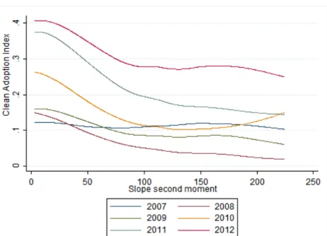
we see some quadratic relation between clean harvesting and slope as in Figure 1. The
relation of Clean Adoption Index and slope’s first and second moments can be seen in
Figure 2 and 3.
However, to use slope as an instrument we should satisfy two assumptions: (i) slope
must be related to Clean Adoption Index; and (ii) slope must be uncorrelated to the
error term. In other words, slope must be correlated with technology adoption and must
be not directly affect the development of local labor markets, except via the mechanized
harvesting. To characterize assumption (i) we show in Figure 2 that Clean Adoption
Index is negatively related to slope first moment, after slope 5, and in Figure 3 that
shows a negative relation between our index and slope second moment.
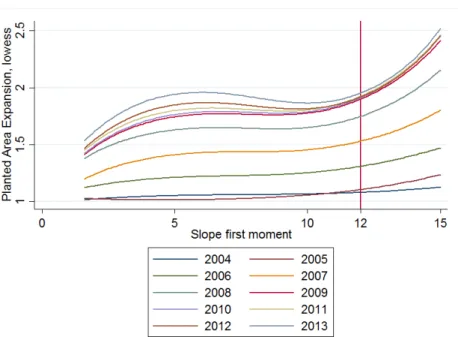
To shed light on the exogeneity assumption (ii), we analyze a panel data of sugarcane
planted area for the whole So Paulo state from 2003 to 2013. Figures 4 and 5 show the
distribution of planted area across different slope levels, wee can see that it does not
change between years. The growth of planted areas, which is defined as planted area at
year t divided by planted area in 2003, is relatively homogeneous across slope levels at
is a uniform across slope first moment. Our intuition for this evidence is that if producers
used to choose more flat terrains to begin with, then slope would be endogenous, but it
seems not to be the case.
Our first stage regression4 equation is:
CleanAdoptionIndexjt = Π1Slopej + Π2Slope2j +λXjt+εjt (4)
whereX was already mentioned, and SlopeandSlope2 are the first and second moments
of land slope at microregion j, respectively. Notice that slope does not change between
years, so were assuming that producers dont make structural changes in terrain, like
terrace for example. In order to avoid for heteroskedasticity and arbitrary intra-group
correlation, serial correlation, we do clustered standard errors at microregion level.
One potential problem that may arise in our regression is the weak instrument
prob-lem. This is the case where slope’s first and second moments are poor predictors of the
Clean Adoption Index. If this is the case, Clean Adoption Index will have little variation
and then will be a bad predictor of our labor market outcomes. We test for weak
in-struments analyzing Kleibergen-Paap F statistic and the Montiel-Pflueger clustered weak
instrument test.
Kleibergen-Paap statistic generalizes the Cragg-Donald statistic to the case of
non-i.i.d. case, in our case we cluster in microregions. It tests whether the instruments
jointly explain enough variation in the multiple endogenous regressors to conduct
mean-ingful hypothesis tests of causal effects. In our case, a single endogenous regressor, the
Kleibergen-Paap Wald F (K-P F) statistic is simply the clustered, first-stage F statistic
(Kleibergen and Paap, 2006).
Weak instruments can bias point estimates and lead to substantial test size
distor-tions. The null hypothesis for Montiel-Pflueger clustered weak instrument test is that the
estimator presents weak instrument bias. The test rejects the null hypothesis when the
test statistic, the effective F statistic, exceeds a critical value. This critical value depends
on the significance level α, and the desired threshold τ. Whereτ is defined as a fraction
of a worst-case benchmark, this benchmark is related with the OLS bias when errors are
conditionally homoskedastic and serially uncorrelated. Montiel-Pflueger clustered weak
4
instrument test can be implemented for multiple instruments but for only one
endoge-nous variable, which is our case, and also supports clustered variance-covariance matrix
estimates (Olea and Pflueger, 2013; Pflueger and Wang, 2014).
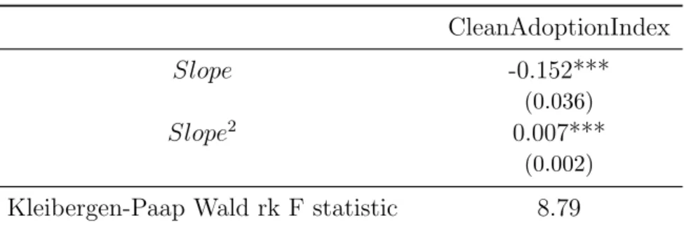
Table 7 presents the first stage results. The sign of our instrumental variables are
different, first moment of land slope is negatively related with our Index, and the second
moment is positively related. Figure 2 and 3 show how Clean Adoption Index is negatively
related with slope first moment, for values greater than 5, and with slope second moment,
respectively. In aggregate we have a negative relation of Slope and Clean Adoption Index.
As can be seen in the table, our K-P F statistic is 8.79 The Montiel-Pflueger clustered
weak instrument test present different values and significance levels for each outcome
variable, but we reject the weak IV bias hypothesis at 20% level for all different outcomes.
After these tests we believe we are not in a weak IV case, so we can go on to interpret
our 2SLS estimates in next section.
4
Empirical Results
We study the effects of environmental regulation and technology adoption on
struc-tural transformation in local labor markets. For this purpose, we analyze the sugarcane
industry in Brazil, more specifically in So Paulo state. In this section, we present the
results of clean harvesting adoption in Brazilian sugarcane industry on local labor
mar-ket outcomes, discussing potential OLS biases caused by endogeneity, and analyzing the
causal estimates from our 2SLS approach.
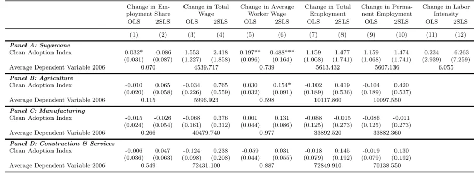
Table 8 presents the main OLS and 2SLS results of equation 3, dividing by sectors
with a total of four panels. We report the coefficient of Clean Adoption Index, clustered
standard errors and the mean of each dependent variable in 2006, the first of our data
basis. The unit of observation is a microregion-year, and all regressions are controled
with year effects and total harvest in 2006 and clean harvesting in 2006.
In terms of comparison we will discuss columns 1 and 2. For Panel A, which presents
the results for sugarcane industry, OLS and 2SLS coefficients present different signs. In
OLS, when we have more clean harvesting we have an increase in Employment Share,
however in 2SLS the effect is the opposite. The 2SLS estimates show suggest that the
Labor intensity is studied only for sugarcane, we do not analyze planted or harvest
area for other cultures. The coefficient of our 2SLS estimate, presented in column 12, is
not statistically significant but suggests that clean adopting leads to a reduction in labor
intensity, we have less workers per harvested area. One harvest machine may substitute
around eighty hand workers, so even employing more workers the harvested area has
grown more. This can be seen as an increase in worker productivity, because now we
need less workers to harvest bigger areas.
Our first question is if this is a labor saving technical change. We can’t answer this for
sure, however the evidence of a reduction in labor intensity and a reduction in employment
share suggests that sugarcane is employing less workers than other sectors. Therefore, we
find weak evidence that this is a labor saving technical change, we now turn to look if it
led to structural changes in the labor market. We try to see if sugarcane mechanization
changed relations in other sectors, for this we also analyze wages and number of workers
in different sectors, looking for sugarcane mechanization impacts in these outcomes.
Still in Employment Share, columns 1 and 2, in Panel B we also see different signs
for the coefficients of Clean Adoption Index, OLS points to a reduction in employment
share and 2SLS estimation is an increase, concluding that in the Agriculture sector OLS
is negatively biased. For the manufacturing sector we see a negative impact of clean
adoption in employment share and we can see in Panel C see that OLS is positively
biased, computing a smaller effect of clean adoption in OLS than in 2SLS. And, in Panel
D we see another change in the sign of the effect, the OLS estimator is negatively biased,
and the correction with instrumental variable reports a positive estimation.
The way were going to interpret our coefficients is that if we have one unit in clean
adoption index – that is if an unity area with initial production is fully based on
pre-harvest burning technique fully converts to mechanical pre-harvesting – we expect an impact
of 100β% in our dependent variable in relation of its value in 2006. Thus, if our clean
index is zero in 2006 and becomes 1, we expect that our dependent variable changes from
Y2006 to (1 +β)Y2006. The median microregion had a clean adoption index of 0.137, and
the mean microregion had the index of 0.163.
Back to employment share, column 2, in the sugarcane sector we see an impact of
-8,6% in employment share for one unit of our clean adoption index, so if one microregion
employ-ment share of 0.038 at this microregion-year. The impact is in other direction in the
agriculture sector, as presented in Panel B, we estimate an increase in 6.5% of this sector
employment share for one unit of clean adoption index, so we expect an employment
share around 0.029 for a microregion-year that had no clean harvesting and only present
this type of harvesting.
Analyzing Change in Total Wage, column 4, for all sectors we see a positive impact of
clean adoption. The coefficient means that one unit of clean adoption index impacts in
Total Wage by 241.8% in sugarcane, 76.5% in agriculture, 37.6% in manufacturing, and
by 23.8% in construction & services from 2006 value at microregion-year. Thus, if clean
index of one microregion was zero in 2006 and becomes one at some year we expect Total
Wage of the sugarcane sector to more than triple, for example, the increase is around 11
million reais, in 2006 values, in the total amount of wages at microregion-year level.
Column 6 reports the coefficients for Change in Average Worker Wage. For all sectors
the coefficient is positive, so an increase in clean harvesting leads to greater worker wage
when compared to 2006. Coefficients are significant for sugarcane sector, at 1% level, and
for agricultural sector at 10% level. For sugarcane sector, a change in one unit in clean
adoption index leads to an increase, of 48.8% for sugarcane sector, 15.4% for agriculture.
In terms of 2006, the impact of one unit of clean adoption index is an increase of around
R$360 in sugarcane sector, R$92 in agriculture sector.
Analyzing the impact of clean harvesting adoption in number of formal employees
we estimate a reduction in manufacturing sectors, and in other sectors we estimate that
more clean harvesting leads to a greater number of workers. For sugarcane it might
be counterintuitive, but as discussed in background section the sugarcane sector was
characterized by informality in labor market, but with mechanization the number of
formal workers has grown, so its reasonable. We distinguish number of formal employees
between total and permanent. The results are quite the same; we do this as way to observe
if there is a structural change in number of temporary workers, however we have very few
observations of temporary employment making impossible for us to conclude anything for
now. We have no significant coefficients. The coefficient for sugarcane, panel A, means
that a municipality with one in clean adoption index will show an increase of 147.7%
in Total Employment and an increase of 147.4% in Permanent Employment. In terms
2006 and totally adopts clean harvesting will employ 8291 new workers with 8265 being
permanent workers.
With these results together we can answer our two main questions. First, we find
suggestive evidence that sugarcane mechanization is a labor saving technical change.
Second, we find some evidence of a structural change in local labor markets. Sugarcane
mechanization leads to an increase in utilization of formal workers as well with an increase
in their wages. This may represent less labor supply for other sectors, the demand
generated by the new agro-industries affects positively workers via wages in all other
sectors.
5
Robustness Check
In this section we do one robustness check. We redo all our results but disaggregating
at municipality level instead of microregion level.
In order to gain more cross section observations we redo all estimations at
municipality-year level. We maintain in our sample only municipalities where we observe any type
of sugarcane harvest for all years. Three municipalities were dropped out because we
observed harvesting just some years, what could be a error because of aggregation level
we worked in our spatial data. We have a balanced panel of 408 municipalities and 7
years of observation, from 2006 to 2012.
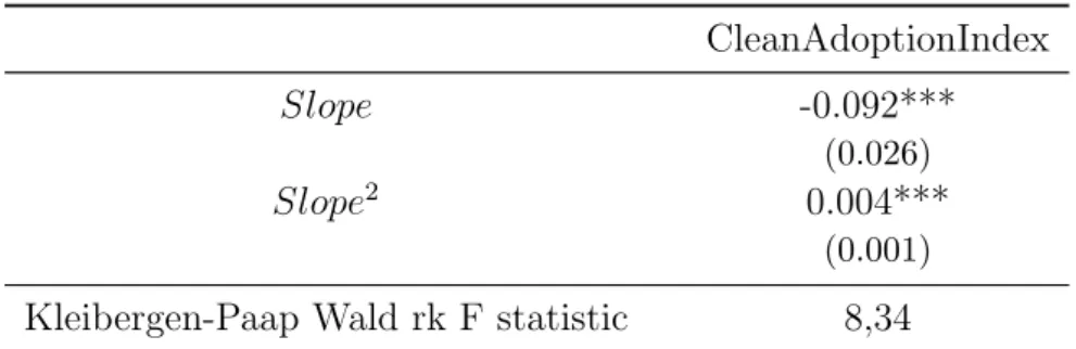
The sign of instrumental variables are according to microregion level estimation, but
the effect is not the same. Here, the first moment of slope distribution has less impact
in clean adoption index. Also we have a smaller K-P F statistic but the Montiel-Pflueger
clustered weak instrument test present different results, in most cases we reject the null
hypothesis at 5% level, but for some we reject only at 20% level.
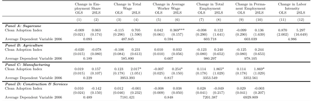
The 2SLS estimation now is quite different from our main estimates. Analyzing Panel
A, wich resumes sugarcane sector coefficients the direction of our causality is different.
For example, at municipality level the clean adoption index coefficient for change in
employment share, column 2, suggests that sugarcane sector is employing more than
other sector, but our main result is the opposite. The same happens with labor intensity
estimative.
because now we only use municipalities where we observe at least one type of sugarcane
harvesting all years, since microregion level data we have more workers in local labor
markets. Also when we make the analysis at the municipality level, we lose a lot of
information because we don’t observe local work migration and or workers commuting.
We can conclude that labor market dynamics at microregion and municipality level are
different, such that what we observe are almost incomparable. One possible cause might
be that for this robustness check we maintain only municipalities that we observe at
least one type of sugarcane harvest, and in our main regression we observe the whole
microregion so we can see migration between municipalities. We understand that a
microregion is a better representation of a local labor market as it considers local economic
complementarity.
6
Conclusion
This paper estimates the causal effects of the adoption of mechanized agriculture led
by a new environmental regulation on local labor markets within a large emerging country,
Brazil.We find that the adoption of clean harvesting leads to a non-significant reduction
in employment share and a non-significant reduction in labor intensity in the sugarcane
sector, that of a labor saving technical change. We find as well that mechanization
increases the number of formal permanent workers and the wage bill in the sugarcane
sector.
We see evidence of structural transformation on labor market by finding that clean
harvesting adoption increases average worker wages in agricultural and manufacturing
sectors. Also, we have suggestive evidence that mechanization in sugarcane harvest
re-duces the number of worker in manufacturing but increases in construction & services
and in agricultural sectors.
Thus we interpret our results as preliminary evidence that mechanization leads to
more formal workers in sugarcane and releases manpower to other cultures, also to
con-struction and services, although this may represent less labor supply to manufacturing.
The demand generated by the new agro-industries affects positively labor market of these
References
Adami, M., M. P. Mello, D. A. Aguiar, B. F. T. Rudorff, and A. F. d. Souza (2012).
A web platform development to perform thematic accuracy assessment of sugarcane
mapping in south-central brazil. Remote sensing 4(10), 3201–3214.
Aguiar, D. A., B. F. T. Rudorff, W. F. Silva, M. Adami, and M. P. Mello (2011). Remote
sensing images in support of environmental protocol: Monitoring the sugarcane harvest
in s˜ao paulo state, brazil. Remote Sensing 3(12), 2682–2703.
Bandiera, O. and I. Rasul (2002, June). Social Networks and Technology Adoption in
Northern Mozambique. STICERD - Development Economics Papers - From 2008 this
series has been superseded by Economic Organisation and Public Policy Discussion
Papers 35, Suntory and Toyota International Centres for Economics and Related
Dis-ciplines, LSE.
Barreca, A., K. Clay, and J. Tarr (2014, February). Coal, Smoke, and Death: Bituminous
Coal and American Home Heating. NBER Working Papers 19881, National Bureau of
Economic Research, Inc.
Beaudry, P., M. Doms, and E. Lewis (2006). Endogenous skill bias in technology adoption:
city-level evidence from the IT revolution. Working Paper Series 2006-24, Federal
Reserve Bank of San Francisco.
Berman, E., J. Bound, and S. Machin (1998, November). Implications Of
Skill-Biased Technological Change: International Evidence. The Quarterly Journal of
Eco-nomics 113(4), 1245–1279.
Braunbeck, O. and P. Magalh˜aes (2010). Avalia¸c˜ao tecnol´ogica da mecaniza¸c˜ao da
cana-de-a¸c´ucar. CORTEZ, LAB Bioetanol de cana-de-a¸c´ucar 1, 451–475.
Bustos, P., B. Caprettini, and J. Ponticelli (2013, August). Agricultural Productivity
and Structural Transformation. Evidence from Brazil. Working Papers 736, Barcelona
Graduate School of Economics.
Can¸cado, J. E., P. H. Saldiva, L. A. Pereira, L. B. Lara, P. Artaxo, L. A. Martinelli,
emissions on the respiratory system of children and the elderly. Environmental health
perspectives, 725–729.
Conley, T. G. and C. R. Udry (2010, March). Learning about a New Technology:
Pineap-ple in Ghana. American Economic Review 100(1), 35–69.
Deschenes, O. (2010, June). Climate Policy and Labor Markets. NBER Working Papers
16111, National Bureau of Economic Research, Inc.
Dominici, F., M. Greenstone, and C. R. Sunstein (2014). Particulate matter matters.
Science (New York, NY) 344(6181), 257.
Esther Duflo, M. K. and J. Robinson (2006, April). Understanding technology adoption:
Fertilizer in western kenya evidence from field experiments. Unpublished working paper.
Foster, A. D. and M. R. Rosenzweig (2010, January). Microeconomics of Technology
Adoption. Working Papers 984, Economic Growth Center, Yale University.
Greenstone, M. (2002, December). The Impacts of Environmental Regulations on
Indus-trial Activity: Evidence from the 1970 and 1977 Clean Air Act Amendments and the
Census of Manufactures. Journal of Political Economy 110(6), 1175–1219.
Greenstone, M. and R. Hanna (2014, October). Environmental Regulations, Air and
Water Pollution, and Infant Mortality in India. American Economic Review 104(10),
3038–72.
Kahn, M. E. and E. T. Mansur (2013). Do local energy prices and regulation affect
the geographic concentration of employment? Journal of Public Economics 101(C),
105–114.
Kleibergen, F. and R. Paap (2006, July). Generalized reduced rank tests using the
singular value decomposition. Journal of Econometrics 133(1), 97–126.
Macedo, I. C., J. E. Seabra, and J. E. Silva (2008). Green house gases emissions in the
production and use of ethanol from sugarcane in brazil: The 2005/2006 averages and
a prediction for 2020. Biomass and bioenergy 32(7), 582–595.
Matsuyama, K. (1992, December). Agricultural productivity, comparative advantage,
Miguel, E. and M. Kremer (2004, 01). Worms: Identifying Impacts on Education and
Health in the Presence of Treatment Externalities. Econometrica 72(1), 159–217.
Novaes, J. R. P. et al. (2007). Jovens migrantes canavieiros: entre a enxada e o fac˜ao.
Relat´orio de estudo desenvolvido para a pesquisa Juventude e integra¸c˜ao sul-americana:
caracteriza¸c˜ao de situa¸c˜oes-tipo e organiza¸c˜oes juvenis, realizada pelo Ibase e pelo
In-stituo P´olis.
Nyko, D., M. S. Valente, A. Y. Milanez, A. K. R. Tanaka, and A. V. P. Rodrigues (2013).
A evolu¸c˜ao das tecnologias agr´ıcolas do setor sucroenerg´etico: estagna¸c˜ao passageira
ou crise estrutural? BNDES Setorial, n. 37, mar. 2013, p 399-442.
Olea, J. L. M. and C. Pflueger (2013, July). A Robust Test for Weak Instruments. Journal
of Business & Economic Statistics 31(3), 358–369.
Pflueger, C. and S. Wang (2014). A robust test for weak instruments in stata. Stata
Journal (forthcoming).
Rangel, M. A. and T. Vogl (2015). The dirty side of clean fuel: Sustainable development,
pre-harvest sugarcane burning and infant health in brazil. mimeo.
Rudorff, B. F. T., D. A. Aguiar, W. F. Silva, L. M. Sugawara, M. Adami, and M. A.
Moreira (2010). Studies on the rapid expansion of sugarcane for ethanol production in
s˜ao paulo state (brazil) using landsat data. Remote sensing 2(4), 1057–1076.
SGPR (2009). Compromisso nacional para aperfei¸coar as condi¸c˜oes de trabalho na cana
de a¸cucar. Technical report, Secretaria Geral da Presidˆencia da Republica.
Walter, A., M. V. Galdos, F. V. Scarpare, M. R. L. V. Leal, J. E. A. Seabra, M. P.
da Cunha, M. C. A. Picoli, and C. Ortol (2014, 01). Brazilian sugarcane ethanol:
developments so far and challenges for the future. Wiley Interdisciplinary Reviews:
Notes: The figure presents clean harvesting in year t divided by clean harvesting in 2006 per value
of slope first moment. To do this we round slope first moment to the first decimal place, so we have more observations at one slope first moment point. We drop slope first moment values greater than 15% because of very few observations.
Figure 1: Clean Harvesting vs Slope first moment
Notes: The figure presents clean adoption index in year t per value of slope first moment, locally
weighted scatterplot smoothing (lowess). To do this we round slope first moment to the first decimal place and then calculate clean adoption index at each rounded value and each yeart. We drop slope first
moment values greater than 15% because of very few observations.
Notes: The figure presents clean adoption index in year t per value of slope second moment, locally
weighted scatterplot smoothing (lowess). To do this we round slope first moment to the first decimal place and then calculate rounded slope second moment, so we calculate clean adoption index at each rounded value and each yeart. We drop slope first moment values greater than 15% because of very few
observations.
Figure 3: Clean Adoption Index vs Slope second moment
Notes: The figure presents presents planted area in yeartdivided by clean harvesting in 2003 per value
of slope first moment. To do this we round slope first moment to the first decimal place, so we have more observations at one slope first moment value. We drop slope first moment values greater than 15% because of very few observations.
Notes: The figure presents presents planted area in yeartdivided by clean harvesting in 2003 per value
of slope first moment, locally weighted scatterplot smoothing (lowess). To do this we round slope first moment to the first decimal place, so we have more observations at one slope first moment value. We drop slope first moment values greater than 15% because of very few observations.
Table 1: Sugarcane Production (thou-sands ton)
Year Brazil So Paulo %
2006 427,723 264,339 62
2007 495,723 296,243 60
2008 569,216 346,293 61
2009 602,193 361,261 60
2010 620,409 359,503 58
2011 559,215 304,230 54
2012 588,478 329,923 56
Notes: The table presents sugarcane production in thousands of ton from Brazil and So Paulo state. Source:UNICADATA
Table 2: Timeline
Year Mechanizable Areas Non-mechanizable Areas
2002 20% reduction
2006 30% reduction
2011 50% reduction 10% reduction
2016 80% reduction 20% reduction
2021 100% reduction 30% reduction
2026 50% reduction
2031 100% reduction
Notes: The table resumes the reduction timeline to end sugarcane pre-harvest burning.
Table 3: Mechanical Harvesting Evolution (%)
Center-South 2006 2007 2008 2009 2010 2011 2012
Mechanical Harvesting 36,7 42,8 53,4 60,1 72,8 79,2 85,1
Green 25,1 29,9 38,2 42,9 52,5 66,3 73,8
Burning 11,6 12,9 15,2 17,1 20,3 13,0 10,8
Hand Harvesting 63,3 57,2 46,6 39,9 27,2 20,8 14,9
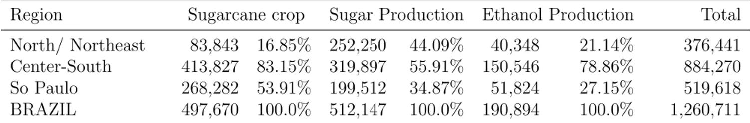
Table 4: Employees in the Sugarcane Industry (2007)
Region Sugarcane crop Sugar Production Ethanol Production Total
North/ Northeast 83,843 16.85% 252,250 44.09% 40,348 21.14% 376,441
Center-South 413,827 83.15% 319,897 55.91% 150,546 78.86% 884,270
So Paulo 268,282 53.91% 199,512 34.87% 51,824 27.15% 519,618
BRAZIL 497,670 100.0% 512,147 100.0% 190,894 100.0% 1,260,711
Notes: This table presents formal workers in sugarcane industry in Brazil at 2007, differentiating between workers of sugarcane crop, sugar production, and ethanol production.
Source: SGPR (2009)
Table 5: Descriptive Statistics: Independent Variables
Mean Median
Slope 7.255 6.984
(1.657)
Slope2 61.895 55.164
(32.740)
Harvest Area 2006 951.932 685
(896.834)
Clean 2006 314.136 210
(314.615)
Clean Adoption Index 0.189 0.167
(0.177)
Table 6: Descriptive Statistics: Dependent Variables
Employment Total Average Total Permanent Labor
Share Wage Worker Wage Employment Employment Intensity
Level Dif Level Dif Level Dif Level Dif Level Dif Level Dif
(1) (2) (3) (4) (5) (6) (7) (8) (9) (10) (11) (12)
Panel A: Sugarcane
Mean 0.055 -0.015 5407.420 867.703 1.045 0.306 4933.127 -680.305 4930.422 -676.714 4.172 -1.883
Std. Deviation (0.063) (0.033) (6023.102) (2321.949) (0.298) (0.264) (5300.260) (2260.568) (5298.576) (2260.522) (3.645) (2.731)
Median 0.035 -0.003 3353.150 285.604 1.015 0.260 2911 0 2911 0 3.022 -0.991
Panel B: Agriculture
Mean 0.104 -0.011 8418.621 2421.698 0.826 0.228 10365.270 247.4026 10358.160 260.6169
Std. Deviation (0.065) (0.023) (7164.818) (3387.854) (0.206) (0.186) (8637.834) (2040.833) (8634.894) (2039.943)
Median 0.085 -0.006 6321.076 1325.303 0.786 0.202 8350 150 8350 148
Panel C: Manufacturing
Mean 0.271 0.005 60286.140 19806.400 1.243 0.266 40323.310 6430.782 40301.620 6419.260
Std. Deviation (0.080) (0.029) (109006.300) (42633.630) (0.343) (0.218) (52479.550) (10555.390) (52455.590) (10541.360)
Median 0.260 0 29096.670 7918.585 1.207 0.243 24014 2815.5 24014 2815.5
Panel D: Construction & Services
Mean 0.571 0.021 115452 43020.880 1.121 0.234 91861.850 19011.940 89157.260 19018.710
Std. Deviation (0.093) (0.039) (229421.900) (109766.600) (0.227) (0.199) (149161.800) (43690.580) (140976.900) (43372.740)
Median 0.569 0.013 52982.990 14980.480 1.089 0.209 47487.5 7412 45885 7522
Notes: The table reports descriptive statistics of dependent variables used in regressions. Variables in level are considered all observations at microregion level between 2006 and 2012. Variables in difference are calculated at microregion level taking the difference between yeartand 2006, wheretis from 2007 to 2012.
Table 7: First Stage
CleanAdoptionIndex
Slope -0.152***
(0.036)
Slope2 0.007***
(0.002)
Kleibergen-Paap Wald rk F statistic 8.79
Table 8: OLS and 2SLS
Change in Em- Change in Total Change in Average Change in Total Change in Perma- Change in Labor
ployment Share Wage Worker Wage Employment nent Employment Intensity
OLS 2SLS OLS 2SLS OLS 2SLS OLS 2SLS OLS 2SLS OLS 2SLS
(1) (2) (3) (4) (5) (6) (7) (8) (9) (10) (11) (12)
Panel A: Sugarcane
Clean Adoption Index 0.032* -0.086 1.553 2.418 0.197** 0.488*** 1.159 1.477 1.159 1.474 0.234 -6.263
(0.031) (0.087) (1.227) (1.858) (0.096) (0.164) (1.068) (1.741) (1.068) (1.741) (2.939) (7.259)
Average Dependent Variable 2006 0.070 4539.717 0.739 5613.432 5607.136 6.055
Panel B: Agriculture
Clean Adoption Index -0.010 0.065 -0.034 0.765 0.030 0.154* -0.102 0.419 -0.104 0.420
(0.020) (0.058) (0.226) (0.559) (0.032) (0.091) (0.189) (0.536) (0.189) (0.537)
Average Dependent Variable 2006 0.115 5996.923 0.598 10117.860 10097.550
Panel C: Manufacturing
Clean Adoption Index -0.015 -0.026 -0.068 0.376 0.001 0.131 -0.088 -0.015 -0.086 -0.011
(0.024) (0.054) (0.161) (0.312) (0.044) (0.086) (0.125) (0.273) (0.125) (0.273)
Average Dependent Variable 2006 0.266 40479.740 0.977 33892.520 33882.360
Panel D: Construction & Services
Clean Adoption Index -0.006 0.047 -0.124 0.238 -0.059 0.031 -0.018 0.145 -0.019 0.130
(0.036) (0.063) (0.098) (0.208) (0.044) (0.055) (0.079) (0.192) (0.079) (0.192)
Average Dependent Variable 2006 0.549 72431.100 0.887 72849.910 70138.550
Notes: The table reports OLS and 2SLS results of equation 3 in the text. The unit of observation is microregion-year. Clustered standard errors at microregion level are reported in brackets. We have 44 microregions and 6 years. All outcomes are in difference with 2006 value. Employment Share and Labor Intensity are fraction, and all other variables are in log. All regressions have year effects and are controled for total harvest in 2006 and clean harvesting in 2006. Significance level: ***p¡0.01, **p¡0.05, *p¡0.10.
Table 9: Municipality Robustness Check: First Stage
CleanAdoptionIndex
Slope -0.092***
(0.026)
Slope2 0.004***
(0.001)
Kleibergen-Paap Wald rk F statistic 8,34
Table 10: Municipality Robustness Check: OLS and 2SLS
Change in Em- Change in Total Change in Average Change in Total Change in Perma- Change in Labor
ployment Share Wage Worker Wage Employment nent Employment Intensity
OLS 2SLS OLS 2SLS OLS 2SLS OLS 2SLS OLS 2SLS OLS 2SLS
(1) (2) (3) (4) (5) (6) (7) (8) (9) (10) (11) (12)
Panel A: Sugarcane
Clean Adoption Index -0.009 0.063 -0.115 0.705 0.042 0.369*** -0.098 0.122 -0.099 0.136 0.870 5.297
(0.021) (0.174) (0.290) (1.590) (0.061) (0.157) (0.290) (1.641) (0.290) (1.639) (2.002) (16.649)
Average Dependent Variable 2006 0.093 487.845 0.594 603.718 603.039 4.986
Panel B: Agriculture
Clean Adoption Index -0.020 -0.078 -0.106 0.231 0.010 0.032 -0.123 0.240 -0.125 0.244
(0.015) (0.080) (0.084) (0.613) (0.010) (0.056) (0.080) (0.652) (0.080) (0.653)
Average Dependent Variable 2006 0.189 585.890 0.607 980.297 978.105
Panel C: Manufacturing
Clean Adoption Index 0.019 0.157 0.123 2.017* -0.007 0.254* 0.114 1.865* 0.114 1.869*
(0.015) (0.107) (0.178) (1.051) (0.025) (0.150) (0.178) (1.029) (0.178) (1.029)
Average Dependent Variable 2006 0.229 3953.393 0.817 3353.549 3352.561
Panel D: Construction & Services
Clean Adoption Index 0.010 -0.142 0.012 -0.001 -0.008 0.038 0.028 -0.049 0.029 -0.003
(0.024) (0.150) (0.046) (0.232) (0.009) (0.050) (0.041) (0.217) (0.041) (0.207)
Average Dependent Variable 2006 0.489 7181.421 0.848 7201.387 6929.809
Notes:The table reports OLS and 2SLS results of equation 3 in the text. The unit of observation is municipality-year. Clustered standard errors at microregion level are reported in brackets. We have 2448 municipalities, 6 years and 44 microregions. All outcomes are in difference with 2006 value. Employment Share and Labor Intensity are fraction, and all other variables are in log. All regressions have year effects and are controled for total harvest in 2006 and clean harvesting in 2006. Significance level: ***p¡0.01, **p¡0.05, *p¡0.10.
A
Appendix
This appendix contains first stage results considering only slope first moment as
in-strument. Table 11 reports coefficient and K-P F statistic. The coefficient sign is still
negative, but we lose in statistical significance and in relevance, the estimated parameter
is very different, suggesting that we have a missing instrument bias. Also, K-P F statistic
now is only 3.38, smaller than before, and Montiel-Pflueger clustered weak instrument
test do not reject weak instrument bias hypothesis.
Table 11: Only Slope First Moment: First Stage
CleanAdoptionIndex
Slope -0.020*
(0.011)
Kleibergen-Paap Wald rk F statistic 3.38