ESCOLA de PÓS-GRADUAÇÃO em
ECONOMIA
Alexis Maka
On Testing the Phillips Curves, the
IS Curves, and the Interaction
between Fiscal and Monetary
Policies
On Testing the Phillips Curves, the
IS Curves, and the Interaction
between Fiscal and Monetary
Policies
Tese submetida à Escola de Pós-Graduação em Economia da Fundação Getulio Vargas como requisito parcial para a obtenção do grau de Doutor em Econo-mia
Orientador: Fernando de Holanda Bar-bosa
Maka, Alexis
On testing the Phillips curves, the IS curves, and the interaction between fiscal and monetary policies / Alexis Maka. – 2013.
95 f.
Tese (doutorado) - Fundação Getulio Vargas, Escola de Pós-Graduação em Economia. Orientador: Fernando de Holanda Barbosa.
Inclui bibliografia.
1. Phillips, Curva de. 2. Política tributária. 3. Polítca monetária. 4. Modelos
econométricos. I. Barbosa, Fernando de Holanda. II. Fundação Getulio Vargas. Escola de Pós- Graduação em Economia. III. Título.
The process of writing and completing this dissertation has left me indebted to several people. Without their help and support this work would never have seen the light of day. I would like to take this opportunity to express my deepest gratitute towards them.
My main debt of gratitude goes to Fernando de Holanda Barbosa for his superb advice, constant dedication, and unfaltering encouragement.
I wish to thank Elcyon Caiado Rocha Lima for carefully reading my dissertation man-uscript and providing me with many insightful and encouraging suggestions. I would also like to thank Renato Fragelli Cardoso, João Victor Issler, and André Minella for providing me with several detailed and valuable comments. Their help has greatly improved the quality of the dissertation.
I gratefully acknowledge the …nancial support from CAPES.
This dissertation consists of three essays on empirical testing of Phillips curves, IS curves, and the interaction between …scal and monetary policies.
The …rst essay ("Phillips Curves: An Encompassing Test") tests Phillips curves using an autoregressive distributed lag (ADL) speci…cation that encompasses the accelerationist Phillips curve (APC), the New Keynesian Phillips curve (NKPC), the Hybrid Phillips curve (HPC), and the Sticky-Information Phillips curve (SIPC). We use data from the United States (1985Q1–2007Q4) and from Brazil (1996Q1–2012Q2), using the output gap and alternatively the real marginal cost as measure of in‡ationary pressure. The empirical evidence rejects the restrictions implied by the NKPC, the HPC, and SIPC, but does not reject those implied by the APC.
The second essay ("IS Curves: An Encompassing Test") tests IS curves using an ADL speci…cation that encompasses the traditional Keynesian IS curve (KISC), the New Keynesian IS curve (NKISC), and the Hybrid IS curve (HISC). We use data from the United States (1985Q1–2007Q4) and from Brazil (1996Q1–2012Q2). The evidence rejects the restrictions implied by the NKISC and the HISC, but does not reject those of the KISC.
The third essay ("The E¤ects of Fiscal Policy and its Interactions with Monetary Policy in Brazil") analyzes the e¤ects of …scal policy shocks on the dynamics of the economy and the interaction between …scal and monetary policy using structural vector autoregressions (SVARs). We test the Fiscal Theory of the Price Level for Brazil, ana-lyzing the response of public sector liabilities to primary surplus shocks. For the hybrid identi…cation we …nd that it is not possible to distinguish empirically between Ricard-ian (Monetary Dominance) and non-RicardRicard-ian (Fiscal Dominance) regimes. However, using sign restrictions there is some evidence that the government followed a Ricardian (Monetary Dominance) regime from January 2000 to June 2008.
Esta tese é composta por três ensaios sobre testes empíricos de curvas de Phillips, curvas IS e a interação entre as políticas …scal e monetária.
O primeiro ensaio ("Curvas de Phillips: um Teste Abrangente") testa curvas de Phillips usando uma especi…cação autoregressiva de defasagem distribuída (ADL) que abrange a curva de Phillips Aceleracionista (APC), a curva de Phillips Novo Keynesiana (NKPC), a curva de Phillips Híbrida (HPC) e a curva de Phillips de Informação Rígida (SIPC). Utilizamos dados dos Estados Unidos (1985Q1–2007Q4) e do Brasil (1996Q1– 2012Q2), usando o hiato do produto e alternativamente o custo marginal real como me-dida de pressão in‡acionária. A evidência empírica rejeita as restrições decorrentes da NKPC, da HPC e da SIPC, mas não rejeita aquelas da APC.
O segundo ensaio ("Curvas IS: um Teste Abrangente") testa curvas IS usando uma especi…cação ADL que abrange a curva IS Keynesiana tradicional (KISC), a curva IS Novo Keynesiana (NKISC) e a curva IS Híbrida (HISC). Utilizamos dados dos Estados Unidos (1985Q1–2007Q4) e do Brasil (1996Q1–2012Q2). A evidência empírica rejeita as restrições decorrentes da NKISC e da HISC, mas não rejeita aquelas da KISC.
O terceiro ensaio ("Os Efeitos da Política Fiscal e suas Interações com a Política Mon-etária") analisa os efeitos de choques na política …scal sobre a dinâmica da economia e a interação entre as políticas …scal e monetária usando modelos SVARs. Testamos a Teoria Fiscal do Nível de Preços para o Brasil analisando a resposta do passivo do setor público a choques no superávit primário. Para a identi…cação híbrida, encontramos que não é possível distinguir empiricamente entre os regimes Ricardiano (Dominância Monetária) e não-Ricardiano (Dominância Fiscal). Entretanto, utilizando a identi…cação de restrições de sinais, existe evidência que o governo seguiu um regime Ricardiano (Dominância Mon-etária) de janeiro de 2000 a junho de 2008.
Palavras-chave: curva de Phillips; curva IS; teste abrangente; choques de política
1 Introduction 11
2 Phillips Curves: An Encompassing Test 13
2.1 Introduction . . . 13
2.2 Phillips Curves . . . 15
2.2.1 Accelerationist Phillips Curve (APC) . . . 15
2.2.2 New Keynesian Phillips Curve (NKPC) . . . 18
2.2.3 Hybrid Phillips Curve (HPC) . . . 19
2.2.4 Sticky-Information Phillips Curve (SIPC). . . 19
2.3 Autoregressive Distributed Lag (ADL) Phillips Curve . . . 20
2.4 Empirical Evidence: United States (1985Q1–2007Q4) . . . 22
2.5 Empirical Evidence: Brazil (1996Q1–2012Q2) . . . 32
2.6 Concluding Remarks . . . 41
2.A Data Appendix . . . 42
3 IS Curves: An Encompassing Test 43 3.1 Introduction . . . 43
3.2 IS Curves . . . 44
3.2.1 Keynesian IS Curve (KISC) . . . 44
3.2.2 New Keynesian IS Curve (NKISC) . . . 45
3.2.3 Hybrid IS Curve (HISC) . . . 46
3.3 IS Curve: An Encompassing Speci…cation. . . 47
3.4 Empirical Evidence: United States (1985Q1 - 2007Q4) . . . 48
3.5 Empirical Evidence: Brazil (1996Q1 - 2012Q2) . . . 54
3.6 Concluding Remarks . . . 61
3.A Data Appendix . . . 62
4 The E¤ects of Fiscal Policy and its Interactions with Monetary Policy in Brazil 63 4.1 Introduction . . . 63
4.2 An Overview of the Fiscal Theory of the Price Level. . . 65
4.3 Data, Model Speci…cation and Estimation . . . 67
4.4 Model Identi…cation . . . 67
4.4.1 The hybrid approach . . . 68
4.4.2 The sign restrictions approach . . . 73
4.5 Concluding Remarks . . . 79
4.A Data Appendix . . . 80
2.1 In‡ation (U.S.) . . . 23
2.2 Output Gap (U.S.) . . . 23
2.3 Median In‡ation x Headline In‡ation (U.S.) . . . 28
2.4 Labor Share of Income (U.S.) . . . 30
2.5 In‡ation (Brazil) . . . 32
2.6 Output Gap (Brazil) . . . 33
2.7 Real Exchange Rate Gap (Brazil) . . . 34
2.8 Core In‡ation x Headline In‡ation (Brazil) . . . 36
2.9 Labor Share of Income (Brazil) . . . 38
3.1 Output Gap and Real Interest Rate Gap (U.S.) . . . 49
3.2 Public De…cit Gap and Government Expenditure Gap (U.S.) . . . 52
3.3 Ouput Gap (Brazil) . . . 55
3.4 Real Interest Rate Gap (Brazil) . . . 56
3.5 Real Exchange Rate Gap (Brazil) . . . 56
3.6 Public De…cit Gap and Government Expenditure Gap (Brazil) . . . 60
4.1 Contemporaneous causal ordering based on DAGs . . . 70
4.2 IRFs with 68% probability bands, using the contemporaneous causal or-dering of Figure 1 to identify the SVAR (24 months ahead) . . . 72
4.3 IRFs based on the hybrid identi…cation (24 months ahead), with 68% prob-ability . . . 74
4.4 IRFs based on the hybrid identi…cation (60 months ahead), with 68% prob-ability bands . . . 75
4.5 IRFs based on the sign restrictions identi…cation (24 months ahead), with 68% probability bands . . . 77
2.1 Model Typology . . . 21
2.2 Unit Root Test for In‡ation (U.S.) . . . 22
2.3 Endogeneity Test for Output Gap (U.S.) . . . 24
2.4 Unrestricted ADL Phillips Curve (U.S.). . . 25
2.5 Restricted ADL Phillips Curve (U.S.) . . . 26
2.6 Wald Test of Coe¢cient Restrictions (U.S.). . . 27
2.7 Unit Root Test for Median In‡ation (U.S.) . . . 27
2.8 Unit Root Test for the …rst di¤erence of Median In‡ation (U.S.) . . . 28
2.9 Endogeneity Test for Output Gap when median in‡ation is used (U.S.) . . 28
2.10 Restricted ADL Phillips Curve, using median in‡ation (U.S.) . . . 29
2.11 Wald Test of Coe¢cient Restrictions when median in‡ation is used (U.S.) . 29 2.12 Endogeneity Test for Labor Share (U.S.) . . . 29
2.13 Restricted ADL Phillips Curve using labor income share (U.S.). . . 30
2.14 Endogeneity Test for Labor Share when median in‡ation is used . . . 30
2.15 Restricted ADL Phillips Curve using median in‡ation and labor income share (U.S.) . . . 31
2.16 Unit Root Test for In‡ation (Brazil) . . . 33
2.17 Endogeneity Test for Output Gap and Real Exchange Rate Gap (Brazil) . 33 2.18 Unrestricted ADL Phillips Curve (Brazil) . . . 34
2.19 Restricted ADL Phillips Curve (Brazil) . . . 35
2.20 Unit Root Test for Core In‡ation (Brazil) . . . 36
2.21 Unit Root Test for the …rst di¤erence of Core In‡ation (Brazil). . . 37
2.22 Endogeneity Test for Output Gap and Real Exchange Rate Gap (Brazil) . 37 2.23 Restricted ADL Phillips Curve using core in‡ation (Brazil) . . . 37
2.24 Endogeneity Test for Labor Share and Real Exchange Rate Gap when headline in‡ation is used . . . 38
2.25 Restricted ADL Phillips Curve using labor share (Brazil) . . . 39
2.26 Endogeneity Test for Labor Share and Real Exchange Rate Gap when core in‡ation is used . . . 39
2.27 Restricted ADL Phillips Curve using core in‡ation and labor share (Brazil) 40 3.1 Model Typology . . . 48
3.2 Endogeneity Test for Real Interest Rate Gap (U.S.) . . . 50
3.3 Unrestricted ADL IS Curve (U.S.). . . 50
3.4 Restricted ADL IS Curve (U.S.) . . . 51
3.5 Endogeneity Test for Real Interest Rate Gap, Government Expenditure Gap, Public De…cit Gap (U.S.) . . . 52
3.8 Restricted ADL IS Curve when public de…cit gap is added to the baseline
model (U.S.). . . 54
3.9 Endogeneity Test for Real Interest Rate Gap and Real Exchange Rate Gap (Brazil) . . . 55
3.10 Unrestricted ADL IS Curve (Brazil) . . . 57
3.11 Restricted ADL IS Curve (Brazil) . . . 58
3.12 Restricted ADL IS Curve when Autometrics is employed (Brazil) . . . 59
3.13 Endogeneity Test for Real Interest Rate Gap, Real Exchange Rate, Gov-ernment Expenditure Gap, Public De…cit Gap (Brazil) . . . 59
3.14 Restricted ADL IS Curve when government expenditures gap and the pub-lic de…cit gap are added to the baseline model (Brazil) . . . 60
4.1 Sign restrictions used to identify the SVAR model . . . 73
Introduction
In the 1970s, 1980s, and early 1990s, models used for monetary policy analysis com-bined the assumption of nominal rigidity with a simple structure that linked the quantity of money to aggregate spending. Although the theoretical foundations of these models were weak, the approach proved remarkably useful in addressing a wide range of monetary policy topics. Today, the standard approach in monetary economics and monetary policy analysis incorporates nominal wage or price rigidity into a dynamic stochastic general equilibrium (DSGE) framework that is based on optimizing behavior by the agents in the model.
These modern DSGE models with nominal frictions are commonly labeled New Keyne-sian models because, like older versions of models in the KeyneKeyne-sian tradition, aggregate demand plays a central role in determining output in the short run, and there is a pre-sumption that some ‡uctuations both can be and should be dampened by countercylical monetary.
In its simplest form the canonical New Keynesian model is composed by: (1) an in‡ation equation, which resembles an expectations-augmented Phillips curve [the New Keynesian Phillips curve]; (2) Euler equation for output, which generalizes the consump-tion Euler equaconsump-tion to the whole economy [the New Keynesian IS curve] ; (3) an equaconsump-tion describing how interest rate policy is set, usually described as an explicit interest rate rule.
The New Keynesian model became the workhorse model for monetary analysis.1
How-ever, to use this model for policy analysis requires it to have a good …t to the data. The …rst two essays of this dissertation are concerned with the econometric analysis of the New Keynesian model.
The …rst essay ("Phillips Curves: An Encompassing Test") tests Phillips curves using an autoregressive distributed lag (ADL) speci…cation that encompasses the Accelerationist Phillips curve (APC), the New Keynesian Phillips curve (NKPC), the Hybrid Phillips curve (HPC), and the Sticky-Information Phillips curve (SIPC). We use data from the United States (1985Q1–2007Q4) and from Brazil (1996Q1–2012Q2), using the output gap and alternatively the real marginal cost as measure of in‡ationary pressure.
The second essay ("IS Curves: An Encompassing Test") tests IS curves using an ADL speci…cation that encompasses the traditional Keynesian IS curve (KISC), the New Keynesian IS curve (NKISC), and the Hybrid IS curve (HISC). We use data from the
1According to table C of Hammond (2010), 20 out of 27 in‡ation targeting central banks either use
United States (1985Q1–2007Q4) and from Brazil (1996Q1–2012Q2).
The distinguishing feature of these essays is the empirical strategy followed that allows us to test di¤erent theoretical models within the same empirical framework. The empirical strategy begins with the formulation of a statistical model that encompasses alternative Phillips (IS) curve models as special cases–the unrestricted ADL Phillips (IS) curve model. The unrestricted ADL model speci…cation takes the following general form in a closed economy:
yt= m
X
s=1
s yt s+ n
X
s=0
szt s+ 1yt 1+"t
Each Phillips (IS) curve model implies restrictions on the set of parameters
( 1; :::; m; 0; :::; n; 1). The empirical strategy proceeds by estimating the unrestricted ADL model and reducing it based on statistical criteria. Finally, we test each Phillips (IS) curve model by comparing its implied restrictions with the values of the estimated parameters of the restricted ADL model.
Recently, there has been a worldwide movement toward the adoption of a policy regime in which the central bank is assigned the task of achieving an in‡ation target. At the same time, the independence of central banks to pursue this goal has also increased, suggesting that the choice of monetary policy to achieve the in‡ation target is a problem that can, and in fact ought to be, separated from the choice of …scal policy or any other public policy. While there is an agreement between most economists regarding the e¤ects of monetary policy shocks, the empirical literature has struggled so far to provide robust stylized facts on the e¤ects of …scal policy shocks. In particular, there is no agreement on even the qualitative e¤ects of …scal policy shocks on macroeconomic variables.
The third essay ("The E¤ects of Fiscal Policy and its Interactions with Monetary Policy in Brazil") analyzes the e¤ects of …scal policy shocks on the dynamics of the eco-nomy and the interaction between …scal and monetary policy in Brazil.2 It uses a
struc-tural vector autoregression (SVAR) model and the test proposed by Canzoneri, Cumby, and Diba (2001). The SVAR is identi…ed by two alternative methodologies. The …rst methodology uses sign restrictions on impulse responses of the exogenous disturbances. The second methodology, developed by Lima, Maka, and Alves (2011) [LMA], combines sign restrictions with restrictions on the contemporaneous causal interrelationships among variables derived by Directed Acyclic Graphs (DAGs). LMA analysis is concerned mainly with the identi…cation of the e¤ects of monetary policy and exchange rate shocks, so no attention was given to …scal policy. In this paper, we extend LMA analysis introducing a set of …scal variables (budget surplus and public sector liabilities) in their VAR model. The hybrid identi…cation strategy pursued consists of two steps. In the …rst step, we use DAGs to select over-identifying restrictions on the contemporaneous coe¢cients based on the conditional independence relations between the variables. These over-identifying restrictions allow us to identify monetary policy and demand shocks and to restrict the co-variance matrix of the reduced-form residuals. In the second step, maintaining restricted the covariance matrix of reduced-form residuals, we keep the identi…ed monetary policy and demand shocks, and impose sign restrictions on the impulse response functions on the other three shocks to identify the …scal policy, supply, and exchange rate shocks.
2This paper is a joint work with Elcyon Caiado Rocha Lima and Amadeu Pumar. It was published
Phillips Curves: An Encompassing
Test
2.1 Introduction
The empirical evidence shows that in‡ation tends to be pro-cyclical: periods of above average in‡ation tend to be associated with above average economic activity. This stat-istical relationship is known as the Phillips curve. The Phillips curve was perceived in the 60’s as a menu for monetary policymakers: they could choose between high in‡ation and low unemployment or low in‡ation and high unemployment. But this interpretation of the Phillips curve assumed that the relationship between unemployment and in‡ation was stable and would not break down once a policymaker attempts to exploit the tradeo¤. After Friedman’s (1968) paper and the high in‡ation episodes experienced by many eco-nomies in the 1970s, this interpretation of the Phillips curve was discredited. After a period of low in‡ation in the 1980s and early 1990s, economists have again worked on a theoretical framework for the Phillips curve. The New Keynesian Phillips curve (NKPC) provides an interpretation of the short-run in‡ation-unemployment trade-o¤ by deriving it from an optimizing framework featuring rational expectations and nominal rigidities. This is a structural model, designed to be capable of explaining the behavior of in‡ation without being subject to the Lucas critique. The NKPC is part of the New Keynesian model which is the workhorse model for monetary analysis. However, to use the NKPC for policy analysis requires it to have a good econometric track record in describing in‡ation dynamics.
This paper tests Phillips curves using an autoregressive distributed lag (ADL) spe-ci…cation that encompasses the accelerationist Phillips curve (APC), the New Keynesian Phillips curve (NKPC), the Hybrid Phillips curve (HPC), the Sticky-Information Phillips curve (SIPC). We use data from the United States (1985Q1–2007Q4) and from Brazil (1996Q1–2012Q2), using the output gap and alternatively the real marginal cost as meas-ure of in‡ationary pressmeas-ure.1 The empirical evidence rejects the restrictions implied by
the NKPC, the HPC, and SIPC, but does not reject those implied by the APC.
A large body of research has used time series methods to estimate the NKPC. Initial attempts to estimate the NKPC using aggregate time series data for the U.S. were not very successful [Galí and Gertler (1999), GG henceforth]: the estimated coe¢cient on the output gap (proxied by detrended real GDP) was small and often negative in quarterly
1Given that we estimate reduced-form models, the choice of the sample in both countries is motivated
data. One interpretation for the poor results using a standard output gap measure is that it is simply a poor proxy for real marginal cost, which according to the theory, would be the appropriate variable. GG report evidence in favor of the New Keynesian Phillips curve when labor’s share of income, rather than a standard output gap variable, is used to proxy for real marginal cost. In order to capture the in‡ation persistence found in the data, GG modify the basic Calvo model of sticky prices to introduce lagged in‡ation into the Phillips curve, called hybrid Phillips curve. Based on U.S. data and using real marginal cost as the forcing variable, GG conclude that not only the forward looking behavior is predominant but, given the small estimate of the degree of backwardness, the pure forward looking model may do a reasonably good job of describing the data. Following the steps of GG, Galí, Gertler and López-Salido (2001) provided evidence on the …t of the NKPC for the Euro area.
Rudd and Whelan (2007) in a critical review of the New Keynesian model argue that the labor’s share version of the model actually provides a very poor description of observed in‡ation behavior. This failure of the model extends along two dimensions: …rst, labor’s share fails to provide a good measure of in‡ationary pressures; and second, this version of the model cannot account for the important role played by lagged in‡ation in empirical in‡ation regressions. They provide an alternative interpretation of the empirical estimates obtained from the hybrid Phillips curve, and argue that the data actually provide very little evidence of an important role for forward-looking behavior of the sort implied by these models.
As an alternative to the models of sticky prices, Mankiw and Reis (2002) [MR] ar-gue that sticky information—the slow dispersion of information about macroeconomic conditions—can help account for the sluggish adjustment of prices and for the real e¤ects that occur in response to monetary shocks. Kiley (2007) attempted to test the sticky in-formation model of in‡ation against the sticky price for the United States using maximum-likelihood techniques. He …nds that, once hybrid-behavior is allowed, hybrid sticky-price models provide a better description of in‡ation dynamics than a sticky-information model. In a small open-economy exchange-rate movements play an important role in the transmission process that links monetary disturbances to output and in‡ation movements. Economic disturbances that originate in other countries have to be taken into account in monetary policy design that are absent in a closed-economy environment. In addition, part of the intermediate inputs are imported from abroad, which consist mainly of raw materials and energy. Usually the prices of imported inputs are more variable than those from domestic labor as well as domestically produced intermediate inputs. This should— other things equal—induce …rms to change their prices more frequently and possibly also by a larger amount in response to more variable input costs. Price setting is also more complex as the choice of currency, competition from abroad and the pass-through of exchange rate changes into prices become an issue. It is therefore not surprising that model building becomes increasingly di¢cult when it comes to modelling in‡ation dynamics in an open economy where the relationship between in‡ation and exchange rate is a key concern.
in the speci…cation with the output gap contrasts with theory and although the impact of the estimate associated with the marginal cost is negligible, it is statistically signi…c-ant. They …nd a small direct impact of the variables associated with economic openness, with the sum of their coe¢cients being close to zero. However, the indirect impact is signi…cant, consistently changing the weights associated with lagged in‡ation and the ex-pected future in‡ation. Mazali and Divino (2010) apply for Brazil the new Keynesian model of Blanchard and Galí (2007) with real wage rigidity and supply shocks. As the estimated coe¢cients satis…ed a set of restrictions imposed by the theoretical model and over-identifying restrictions were not rejected, they concluded that the estimated New Keynesian Phillips curve adjusted very well to the Brazilian data.2
The paper is organized as follows. Section 2 reviews the literature on Phillips curves. Section 3 presents the ADL Phillips curve and shows how the di¤erent Phillips curve speci…cations considered in the literature can be seen as special cases of the ADL Phillips curve. Section 4 tests for the U.S. the restrictions implied by the di¤erent Phillips curve speci…cations. Section 5 estimates the ADL Phillips curve for Brazil and tests the …t of the alternative models. Finally, section 6 brings the concluding remarks.
2.2 Phillips Curves
In a seminal paper, Phillips (1958) showed that there was a negative and relatively stable relationship between nominal wage in‡ation and unemployment in the United King-dom over the previous century. This relationship was found to work well for price in‡ation and for other economies, receiving the name of "Phillips curve". It became a key part of the standard Keynesian textbook model of the 1960s and as Keynesian economists saw it, the Phillips curve provided an exploitable tradeo¤ between in‡ation and unemployment: policy-makers could use demand management policies to increase output and decrease un-employment, but this could only be done at the expense of higher in‡ation. The Phillips curve relationship can be represented as
t= ut; (2.1)
where t is in‡ation, ut is the unemployment rate, and >0.
The theoretical foundations of these early formulations were not completely sound, with a particular weak point being their treatment of how expectations would enter wage and price setting. This weakness was thoroughly criticized in the seminal contributions of Phelps (1967, 1968) and Friedman (1968).
2.2.1 Accelerationist Phillips Curve (APC)
Friedman argued that the correct formulation of the in‡ation-unemployment tradeo¤ was a Phillips curve of the form:
t =Et 1 t (ut u); (2.2)
where in‡ation, t, is negatively correlated with deviations of the unemployment rate from its natural rate u ( > 0) and where the entire curve is shifted up or down one-for-one
2Other articles that estimate the Phillips curve for Brazil include Cysne (1985), Lima (2003), Minella
with changes in the rate of in‡ation that agents expected at timet-1 to prevail at timet,
Et 1 t. A common variant of this equation replaces ut u with the gap between actual and potential output,yt y xt.
Friedman predicted that attempts to keep unemployment low at the expense of higher in‡ation would just result in raised in‡ation expectations. Thus, the economy would not be able to sustain the low unemployment and would end up with higher in‡ation. In the Friedman-Phelps framework, then, there is no permanent tradeo¤ between the level of in‡ation and the unemployment rate—in the long run, Et 1 t = t, and the Phillips curve is vertical at ut =u . However, to the extent that agents’ expectations were slow to catch up with the reality, a policymaker could keep unemployment below the natural rate by constantly boosting the in‡ation rate. For this reason, the Friedman-Phelps characterization of the in‡ation process also came to be known as the “accelerationist hypothesis” since an acceleration in prices (an increase in the rate of in‡ation) would occur should policymakers attempt to permanently keep unemployment below its natural rate. Phelps assumed that in‡ation expectations evolved over time as a result of actual past experience—that is, that expectations were formed adaptively3. There is a long
tradition in applied work that assumes backward-looking expectations: expected in‡ation is determined by past in‡ation. In the special case where Et 1 t = t 1, the Phillips curve becomes
t= t 1 (ut u): (2.3)
This so-called accelerationist Phillips curve—in which the acceleration of prices is related to unemployment—embodied two critical innovations in the literature. First, it eliminated the long-run trade-o¤ between in‡ation and unemployment that was inherent in the original Phillips curve model. Second, it began to emphasize the importance of expectations in the price-setting process, a change that was to have dramatic implications in the evolution of in‡ation models for the next four decades.
In the decade following the publication of the Phelps and Friedman papers, the notion that the accelerationist view of the in‡ation process was correct gained wider acceptance. Several factors contributed to this attitude. The …rst, of course, was the strength of the theoretical arguments themselves. Second, it became apparent by the mid-1970s that the in‡ation-unemployment tradeo¤ implied by the short-run Phillips curve had shifted. Finally, it became easier to …nd that the lags of in‡ation in empirical Phillips curves summed to one. In addition, the important contribution of “supply shocks” to price acceleration in the early 1970s led to food, energy, and/or import prices receiving special treatment in empirical descriptions of in‡ation. What emerged in this period, therefore, was a benchmark econometric model of in‡ation of the form:
t= ut+B(L) t 1+ zt+"t; (2.4)
whereB(L) is the distributed lag operator with B(1) = 1 , zt denotes a vector of supply shocks, and"tis an error term. In this speci…cation, then, in‡ation dynamics are determ-ined by three sources: real activity (as summarized by the unemployment rate), supply shocks, and “inertia” (as captured by the lagged in‡ation terms); for this reason, it is sometimes called the “triangle model”.
The basic framework of the triangle model has been widely adopted by applied mac-roeconomists, and has brought with it the important concept of the NAIRU, de…ned as
3In Phelps (1967), the appeal to adaptive expectations is explicit. The term is not used by Friedman
the unemployment rate consistent with unchanging in‡ation in the absence of supply shocks. In the context of the simple version of the triangle model presented above (equa-tion 4), the NAIRU is calculated from the estimated coe¢cients as u = = . More re…ned analyses of the NAIRU include Staiger, Stock, and Watson’s (1997a) improved approach for quantifying the precision with which the NAIRU can be measured, attempts by Staiger, Stock, and Watson (1997b), Gordon (1998), and Ball and Mankiw (2002) to model variations over time in the NAIRU.
Taken literally, the characterization of in‡ation dynamics that the triangle model provides carries important implications for the conduct of macroeconomic policy. To the extent that lagged in‡ation captures true inertia in the price-setting process (resulting, for instance, from how expectations are formulated), the model implies that rapid reductions in in‡ation can only be produced at the cost of a substantial increase in unemployment. Hence, the model points to a gradualist approach as providing the best way to e¤ect a large reduction in in‡ation. In addition, policymakers must be mindful of the presence of long time lags between macroeconomic shocks (including policy actions) and their full e¤ects on in‡ation. Thus, this framework provides a strong argument in support of preemptive action to cut o¤ the full e¤ect of an in‡ationary shock.
The introduction of rational expectations into the modelling of economic dynamics had a signi…cant in‡uence on the development of macroeconomic theory from the mid-1970s onwards. The “demise” of the traditional Phillips curve, and the sense that it was due to inadequate modelling of expectations, was a major impetus for the rational expectations school led by Robert Lucas and Thomas Sargent. Lucas and Sargent also rejected the “accelerationist” reformulation of the Phillips curve because it relied on the assumption of adaptive expectations, which do not allow for the idea that agents process information in an optimal manner. In addition to being more precise about expectations formation, this school of economists relied more heavily on neoclassical “microfounda-tions” for macroeconomic models. Often, as well as rejecting the Phillips curve, these economists also questioned the whole basis for Keynesian economics, i.e. the assumption that monetary policy could systematically a¤ect output even in the short-run. How-ever, the Lucas supply curve advanced by Lucas (1972)—the so-called “islands” model in which a short-run in‡ation-output tradeo¤ resulted from imperfect information on the part of price-setters—generally failed to convince as a model of economic ‡uctuations. In part, this initial resistance to the rational expectations approach likely re‡ected the Lucas model’s implication that only purely random and transitory policy shocks could a¤ect output
reach certain bounds. In time dependent models, …rms set their prices for …xed periods of time. Time dependent models can have explicit closed-form solutions relating current price changes to future price changes and the current state of demand. State-dependent models do not, in general, have simple closed-form solutions. Many academic economists have become convinced that certain theoretical new Keynesian models can provide a good description of the empirical in‡ation process. In part, this development stemmed from the realization that a number of popular new Keynesian models of price-setting each implied a sort of Phillips curve relationship. We will now describe one of the key New-Keynesian models and explore its implications for the behaviour of in‡ation and output.
2.2.2 New Keynesian Phillips Curve (NKPC)
Three papers that arrived on the scene around the same time provided partial answers to this question regarding the existence of rigid (or“sticky”) wages and prices. Both au-thors, Calvo (1983) and Rotemberg (1982, 1983), o¤ered di¤erent explanatory rationales, but when stripped to their respective cores, their models are nearly identical and bear essentially the same implications for macroeconomic dynamics.
Calvo’s (1983) model of random price adjustment assumes that in each period a ran-dom fraction (1 !) of …rms can adjust their prices, while all the other …rms keep their prices unchanged. The expected time between price adjustments is 1=(1 !) . The evolution of the (log) price level is given by
pt=!pt 1+ (1 !)zt; (2.5)
whereztis the price chosen by those who can adjust their prices. Assuming a monopolistic competition structure such that, absent any frictions, …rms would set their price as a …xed markup over marginal cost, a …rm’s optimal reset price is determined by
zt= (1 ! )
1
X
j=o
(! )jEt(M Ct+j + ); (2.6)
where is the frictionless optimal markup, is the …rm’s discount factor, and M Ct is nominal marginal cost. In other words, …rms take into account that their prices will likely be …xed over some period by setting their price equal to a weighted average of expected future nominal marginal costs. These two equations can be combined to yield a NKPC of the form4:
t= Et t+1+
(1 !) (1 !)
! (mct+ ); (2.7)
which relates current in‡ation to next period’s expected in‡ation rate and the deviation of current real marginal cost (mct) from its optimal frictionless level.
Under relatively general conditions, aggregate real marginal cost is proportional to the gap between output and its potential level5. With this assumption, the NKPC becomes
t= Et t+1+ xt; (2.8)
where xt is a measure of output gap.
4For a detailed derivation of the NKPC, see for example, Walsh (2010).
5In the standard sticky price framework without variable capital, there is an approximate proportionate
In‡ation is determined in a completely forward-looking manner, as can be seen by solving forward equation (2.8) to obtain the following closed-form solution for the "fun-damental"in‡ation6:
t= 1
X
k=o
( )kEt(xt+k): (2.9)
The idea that there is considerable inertia in in‡ation and hence that it is di¢cult to reduce in‡ation quickly, does not hold in this framework— indeed, according to the NKPC, there is no “intrinsic” inertia in in‡ation, in the sense that there is no structural dependence of in‡ation on its own lagged values. Thus, the NKPC has very di¤erent implications for monetary policy. This model implies that there is no need for gradualist policies to reduce in‡ation. According to the NKPC, low in‡ation can be achieved imme-diately by the central bank announcing (and the public believing) that it is committing itself to elminating positive output gaps in the future.
2.2.3 Hybrid Phillips Curve (HPC)
Many estimates of the NKPC …nd that lagged in‡ation helps to explain current in-‡ation. GG consider augmenting the NKPC with a backward-looking element that is motivated by the presence of some …rms that follow a simple rule of thumb in setting prices. Christiano, Eichenbaum, and Evans (2005) derive a similar speci…cation under the assumption that price-setters who are unable to reset prices instead index their prices to the last period in‡ation rate. All of these variants imply a so-called HPC of the form
t= b t 1 + fEt t+1+ xt: (2.10)
If b+ f = 1, then the Phillips curve is vertical in the long-run, that is, there is no long-run tradeo¤ between in‡ation and real activity.
As shown by Barbosa (2013b), the estimates b and f can be misleading indicators of forward- and backward-looking behavior: it is possible to have f > b but the model can in fact be totally backward-looking.
2.2.4 Sticky-Information Phillips Curve (SIPC)
The Mankiw and Reis (2002) [MR] model pioneers the literature on sticky information and argues that a Phillips curve with this rigidity is an adequate representation of the structural relationship between in‡ation and the real side of the economy. MR derives the SIPC based on the assumption that …rms set price freely but the information for setting prices may or may not be updated. Because information constraints could apply to all economic agents, the sticky information model potentially provides a unifying framework for explaining inertial behavior in di¤erent macroeconomic variables.
The SIPC assumes that …rms set their price every period, but …rms gather information and re-compute optimal prices slowly over time. In each period, a fraction of …rms obtains new information about the state of the economy and computes a new path of optimal prices, and(1 ) …rms continue to set prices based on old plans and outdated information.
6In order to get the solution of in‡ation as the present discounted value of outputgaps we assume that lim
T!1
T
P
i=0
i
Etxt+i converges and that lim T!1
T
Each …rm has the same probability of being one of the …rms updating their information sets, regardless of how long it has been since their last update. The expected time between price updates is therefore 1= .
A …rm’s optimal price that maximizes expected pro…ts at any given point in time is
pt =pt+ xt , where pt is the overall price level and xt is the output gap. A …rm that lasts updated its plans j periods ago sets its price as the expected value of the optimal price j periods ago: ztj =Et jpt.
The aggregate price level is the average of the prices of all …rms in the economy, assuming that the arrival of decision dates is a Poisson process given by:
pt= 1
X
j=0
(1 )jztj:
The price level is then de…ned bypt= 1
P
j=0
(1 )jE
t j(pt+ xt), so that, the baseline SIPC is de…ned as:
t= 1
X
j=0
(1 )jEt 1 j( t+ xt) +
1 xt+"t: (2.11)
In this set-up, in‡ation depends on output, past expectations of current in‡ation and past expectations of changes in current output gap growth.
2.3 Autoregressive Distributed Lag (ADL) Phillips
Curve
A model of in‡ation dynamics general enough to encompass the NKPC, the APC, the HPC, and the SIPC as special cases takes the form
t= 1 t 1+ 0xt+ 1xt 1+ 1 t 1+"t: (2.12)
Let us show how each model is embedded in equation (2.12). The simple APC (SAPC) is given by
t= t 1+ xt+"t; which is equivalent to
t= xt+"t:
This is a particular case of equation (2.12) when 1 = 0; 0 = >0; 1 = 1 = 0: When expected in‡ation of the Phillips curve depends on additional in‡ation lags we have the APC. For the case in which expected in‡ation depends on the last two in‡ation lags the APC is given by
t=!1 t 1+!2 t 2+ xt+"t: After some algebra, this can be rearranged as
Assuming that !1 +!2 = 1, that is, there is no long-run trade-o¤ between in‡ation and real activity, then
t= !2 t 1+ xt+"t:
This speci…cation is a particular case of equation (2.12) when 1 = !2 <0; 0 = >0;
1 = 1 = 0:
The NKPC is given by
t = Et t+1+ xt+"t:
Assuming rational expectations,Et t+1 = t+1 t+1 , the NKPC can be written as
t=
1
t 1 xt 1+ t; 6= 0:
This follows from equation (2.12) when 1 = 0 = 0; 1 = = <0; 1 = (1 )= >0: The HPC is given by7
t= b t 1+ fEt t+1+ xt+"t:
As with the NKPC, we assume rational expectations and after some algebra we obtain
t = b f
t 1 f
xt 1+
(1 b f)
f
t 1+ t; f 6= 0:
This is a particular case of equation (2.12) when 1 = b= f >0; 0 = 0; 1 = k= f <0;
1 = (1 b f)= f >0:
The SIPC derived by MR is given by
t= 1
X
j=0
(1 )jEt 1 j( t+ xt) +
1 xt+"t:
Assuming rational expectations and using the lag operatorLjE
t 1 =Et 1 j , we obtain after some algebra the following expression for the acceleration of in‡ation
t =
(2 ) (1 )2 xt
2 (1 )
(1 )2 xt 1+&t; 6= 0:
This expression is a particular case of equation (2.12) when 1 = 0; 0 = (2 )=(1
)2 >0;
1 = 2 (1 )=(1 )2 <0; 1 = 0:
Table 2.1 shows the restrictions implied by each Phillips curve model subsumed by equation (2.12), which is an ADL(1,1). Once the parameters of the model have been estimated –( 1; 0; 1; 1) – table 2.1 enables us to identify which Phillips curve model is consistent with the evidence. For example, if the estimated coe¢cient of t 1( 1) is negative, then only the APC would be consistent with data.
Model Parameters
1 0 1 1
APC - + 0 0
NKPC 0 0 - +
HPC + 0 - +
SIPC 0 + - 0
Table 2.1: Model Typology
The ADL Phillips curve [equation (2.12)] actually encompasses all Phillips curves as special cases. This provides a convenient framework for analysing the properties of each model used in empirical research, highlighting their respective strengths and weaknesses. The unrestricted ADL Phillips curve includes additional lags of both output gap and in‡ation acceleration, according to:
t = m
X
s=1
s t s+ n
X
s=0
sxt s+ 1 t 1+"t: (2.13)
In this paper we test the NKPC against the HPC, the SIPC, and the APC based on the encompassing ADL Phillips curve [equation (2.13)]. The empirical strategy, inspired in the general-to-speci…c approach to econometrics, is as follows: (i) formulate and estimate a Phillips curve model that encompasses the NKPC, the HPC, the SIPC and the APC as special cases—the unrestricted ADL Phillips curve; (ii) reduce the unrestricted ADL Phillips curve model based on statistical criteria—the restricted ADL Phillips curve; (iii) test each Phillips curve model by comparing its implied restrictions with the values of the estimated parameters of the restricted ADL model.8
2.4 Empirical Evidence: United States (1985Q1–2007Q4)
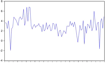
The U.S. sample goes from 1985Q1 to 2007Q4, the period known as "Great Modera-tion"due to the decline in the variability of both output and in‡ation.9 Figure 2.1 plot
the in‡ation rate and table 2.2 shows that it is stationary at the 5% level.10 Figure 2.2
exhibits the output gap.11
Null Hypothesis: In‡ation has a unit root Exogenous: Constant
Lag length: 2 (Spectral OLS AR based on SIC, maxlag=11) Sample: 1985Q1 2007Q4
P-Statistic Elliott-Rothenberg-Stock Point Optimal test statistic 2.074
Test critical values: 1% level 1.937
5% level 3.087 10% level 4.128
Table 2.2: Unit Root Test for In‡ation (U.S.)
8For a survey on the general-to-speci…c modeling see Campos, Ericsson, and Hendry (2005).
9James Stock coined the phrase “the great moderation” while writing a research paper with Mark
Watson in 2002 (“Has the Business Cycle Changed and Why?”). It was brought to the attention of the wider public by Ben Bernanke (then member and now chairman of the Board of Governors of the Federal Reserve) in a speech titled “The Great Moderation” in 2004. The results do not change signi…cantly when we start or …nish the sample one year earlier.
10The Data Appendix gives details on the de…nitions of the variables used in the baseline model and
the robustness analysis.
11Proponents of the New Keynesian model criticize traditional measures of the output gap on the
-4 -2 0 2 4 6 8
1986 1988 1990 1992 1994 1996 1998 2000 2002 2004 2006
Figure 2.1: In‡ation (U.S.)
-4 -3 -2 -1 0 1 2 3 4
1986 1988 1990 1992 1994 1996 1998 2000 2002 2004 2006
Figure 2.2: Output Gap (U.S.)
appropriateness of OLS or the necessity to resort to IV/GMM methods.12 We apply the
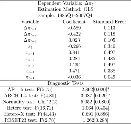
GMM distance test (also known as C test) of a subset of orthogonality conditions to test the endogeneity ofxt.13;14 The endogeneity test displayed on table2.3, indicates that we can treatxtas an exogenous variable.15 Therefore, we proceed with our empirical analysis by estimating the unrestricted ADL Phillips curve [equation (2.13)] using OLS, setting
m=n= 4 [see table 2.4].
Null Hypothesis: Output Gap is exogenous value d.f. Probability Di¤erence in J-statistics 1.085 1 0.297
Table 2.3: Endogeneity Test for Output Gap (U.S.)
12If orthogonality between regressors and the error term cannot be rejected, we should use OLS rather
than IV or GMM, especially in small samples.
13In our context, the GMM distance test of a subset of orthogonality conditions is equivalent to the
Durbin-Wu-Hausman endogeneity test. See Baum, Scha¤er, and Stillman (2003, 2007).
14The GMM distance test is computed as the di¤erence between two J-statistics: that for the
(re-stricted, fully e¢cient) regression using the entire set of overidentifying restrictions, versus that for the (unrestricted, ine¢cient but consistent) regression using a smaller set of restrictions, in which a speci…ed set of instruments is removed from the set. For instruments included in the equation to be estimated, the GMM distance test places them in the list of included endogenous variables; in essence, treating them as endogenous regressors. The GMM distance test, distributed 2 with degrees of freedom equal to the
loss of overidentifying restrictions (i.e., the number of suspect instruments being tested), has the null hypothesis that the speci…ed variables are proper instruments, that is, they are exogenous.
15Given the structure of the error term when the ADL Phillips curve is restricted to be either the
Dependent Variable: t Estimation Method: OLS sample: 1985Q1–2007Q4
Variable Coe¢cient Standard Error
t 1 -0.589 0.113
t 2 -0.422 0.118
t 3 0.023 0.105
xt -0.266 0.340
xt 1 0.841 0.497
xt 2 0.284 0.485
xt 3 -1.294 0.497
xt 4 0.471 0.338
t 1 -0.036 0.049
Diagnostic Tests
AR 1-5 test: F(5,75) 2.862[0.020]* ARCH 1-4 test: F(4,80) 3.087 [0.020]* Normality test: Chi^2(2) 5.052 [0.0800] Hetero test: F(16,71) 1.064 [0.404] Hetero-X test: F(44,43) 0.691 [0.886] RESET23 test: F(2,78) 1.262[0.288]
The values in brackets denote probability values (p-values). Signi…cant diagnostic tests at 5% level are shown by one star.
Table 2.4: Unrestricted ADL Phillips Curve (U.S.)
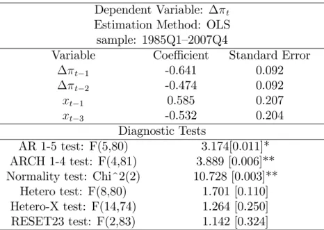
Next, we reduce the unrestricted ADL Phillips curve by sequential elimination of regressors based on t-ratios of the parameters estimators. We sequentially delete those regressors with the smallest t-ratios and re-estimate the model until the t-ratios are all greater than the threshold = 2.16 The resulting restricted ADL model is displayed on
table2.5.
16In a context of VAR models, Brüggemann and Lütkepohl (2001) showed that this strategy is
Dependent Variable: t Estimation Method: OLS sample: 1985Q1–2007Q4
Variable Coe¢cient Standard Error
t 1 -0.641 0.092
t 2 -0.474 0.092
xt 1 0.585 0.207
xt 3 -0.532 0.204
Diagnostic Tests
AR 1-5 test: F(5,80) 3.174[0.011]* ARCH 1-4 test: F(4,81) 3.889 [0.006]** Normality test: Chi^2(2) 10.728 [0.003]**
Hetero test: F(8,80) 1.701 [0.110] Hetero-X test: F(14,74) 1.264 [0.250] RESET23 test: F(2,83) 1.142 [0.324]
The values in brackets denote probability values (p-values). Signi…cant diagnostic tests at 5% level are shown by one star. Signi…cant diagnostic tests at 1% level are shown by two stars.
Table 2.5: Restricted ADL Phillips Curve (U.S.)
According to Table 2.5, the restricted model is composed by the …rst two lags of the change in in‡ation, and the lags of order one and three of the output gap. Using equation (2.12) and comparing the values of Tables 2.1 and 2.5, we observe that only one of the restrictions implied by the SIPC is veri…ed ( 1 = 0). Only one of the restrictions implied by the NKPC and the HPC is accepted ( 0 = 0), while all their other restrictions are rejected by the U.S. data. The APC has two restrictions correct ( 1 <0and 1 = 0) and restrictions on the output gap ( 0 >0 and 1 = 0) that are consistent with the fact that their sum is positive when in‡ation depends on additional lags of output gap.
We conclude that only the APC model is consistent with in‡ation dynamics in the U.S. from 1985Q1–2007Q4. It should be noticed, however, that the diagnostic tests of Table2.5 indicate some misspeci…cation problems with the estimated model, as the hy-pothesis of normality of the distribution of the residuals is rejected, and there is evidence of autocorrelation and conditional heteroscedasticity of the residuals.
The restricted ADL Phillips curve of table 2.5can be written in the Error-Correction form as17
( t) = 2 ( t 1) 3( xt 1+ xt 3) (1 1 2) t 1 1
+ 3 1 1 2
xt 1 +"t
whereh t 1 1 1+1 32xt 1
i
measures the deviation of t 1 from its the long-run solu-tion. Table 2.6 shows that the coe¢cient of xt 1 is not signi…cantly di¤erent from zero, implying that in‡ation depend on output gap changes, not on its level.
17The Error Correction Model (ECM) represents the dynamics in a di¤erent way from the ADL model
Null Hypothesis: ( 1+ 3)=(1 1 2) = 0 value d.f. Probability Chi-square test statistic 0.262 1 0.608
Table 2.6: Wald Test of Coe¢cient Restrictions (U.S.)
Robustness
Since Gordon (1982), many empirical researchers add supply shocks to the Phillips curve. Excluded supply shock variables are positively correlated with in‡ation and pos-itively correlated with the output gap, so the omission of these supply shock variables causes the coe¢cient on the output gap to be biased towards zero. Following Ball and Mazumber (2011), we de…ne core in‡ation as the part of in‡ation explained not by supply shocks. With this de…nition one can measure core in‡ation by removing the e¤ects of supply shocks from total in‡ation. If supply shocks are asymmetries in the distribution of price changes, then a measure of core in‡ation should eliminate the e¤ects of these asym-metries. A simple measure, proposed by Bryan and Cecchetti (1994), is the weighted median of price changes across industries (median in‡ation) [see Figure 2.3]. As a ro-bustness check, we estimate the unrestricted ADL Phillips curve using median in‡ation, instead of the headline in‡ation. Tables2.7 and 2.8 show that median in‡ation is di¤er-ence stationary, which implies that the coe¢cient of lagged in‡ation in equation (2.13) is equal to zero( 1 = 0), whilet-tests are still appropriate to evaluate the other (stationary) variables.18 Table2.10displays the results of the estimated restricted ADL Phillips curve.
With the median in‡ation the lag of order four of the output gap is now relevant, instead of order three, and the values of the coe¢cients are di¤erent. However, we reach the same conclusion as before: the APC is still consistent with in‡ation dynamics in the U.S.. Fur-thermore, the diagnostic tests of Table2.10 indicate that the estimated model performs better when a measure of core in‡ation is used—median in‡ation—suggesting that the omission of supply shocks may be jeopardizing the estimation with headline in‡ation.
Regarding the Error-Correction representation, table 2.11 shows that the coe¢cient measures the deviation of t 1 from its long-run solution is signi…cantly di¤erent from zero, implying that in‡ation depends on the level of the output gap and its changes.
Null Hypothesis: Median In‡ation has a unit root Exogenous: Constant
Lag length: 1 (Spectral OLS AR based on SIC, maxlag=11) Sample: 1985Q1 2007Q4
P-Statistic Elliott-Rothenberg-Stock Point Optimal test statistic 7.790
Test critical values: 1% level 1.937
5% level 3.087 10% level 4.128
Table 2.7: Unit Root Test for Median In‡ation (U.S.)
-4 -2 0 2 4 6 8
1986 1988 1990 1992 1994 1996 1998 2000 2002 2004 2006
Headline Inflation Median Inflation
Figure 2.3: Median In‡ation x Headline In‡ation (U.S.)
Null Hypothesis: (median in‡ation)t has a unit root Exogenous: Constant
Lag length: 1 (Spectral OLS AR based on SIC, maxlag=11) Sample: 1985Q1 2007Q4
P-Statistic Elliott-Rothenberg-Stock Point Optimal test statistic 0.827
Test critical values: 1% level 1.937
5% level 3.087 10% level 4.128
Table 2.8: Unit Root Test for the …rst di¤erence of Median In‡ation (U.S.)
Null Hypothesis: Output Gap is exogenous value d.f. Probability Di¤erence in J-statistics 0.894 1 0.344
Dependent Variable: (median in‡ation)t Estimation Method: OLS
sample: 1985Q1–2007Q4
Variable Coe¢cient Standard Error
(median in‡ation)t 1 -0.648 0.097
(median in‡ation)t 2 -0.308 0.097
xt 1 0.122 0.035
xt 4 -0.071 0.034
Diagnostic Tests
AR 1-5 test: F(5,79) 1.210 [0.312] ARCH 1-4 test: F(4,80) 0.549 [0.700] Normality test: Chi^2(2) 0.630 [0.729] Hetero test: F(8,79) 0.701 [0.689] Hetero-X test: F(14,73) 0.946 [0.514] RESET23 test: F(2,82) 0.976 [0.380]
The values in brackets denote probability values (p-values).
Table 2.10: Restricted ADL Phillips Curve, using median in‡ation (U.S.)
Null Hypothesis: ( 1+ 4)=(1 1 2) = 0 value d.f. Probability Chi-square test statistic 4.563 1 0.032
Table 2.11: Wald Test of Coe¢cient Restrictions when median in‡ation is used (U.S.)
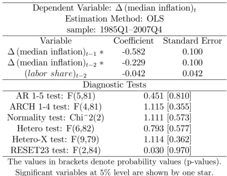
Motivated by the NKPC literature, we also modi…ed the ADL Phillips curve by repla-cing the output gap with the real marginal cost, proxied by the labor share of income (see Figure 2.4).19 The results of the estimated restricted ADL Phillips curve are displayed
on Table 2.13 (for headline in‡ation) and Table 2.15 (for median in‡ation). In none of these cases the labor share of income appears to be a (statistically) relevant variable for explaining in‡ation dynamics. Furthermore, the signs of in‡ation acceleration are con-sistent only with the APC. Once again, the diagnostic tests indicate that the estimated model performs better when median in‡ation is used.
Null Hypothesis: Labor Share is exogenous value d.f. Probability Di¤erence in J-statistics 1.397 1 0.237
Table 2.12: Endogeneity Test for Labor Share (U.S.)
19Most papers in the recent literature on the NKPC have referred to labor’s share of income as real
-2 -1 0 1 2 3 4
1986 1988 1990 1992 1994 1996 1998 2000 2002 2004 2006
Figure 2.4: Labor Share of Income (U.S.)
Dependent Variable: t Estimation Method: OLS sample: 1985Q1–2007Q4
Variable Coe¢cient Standard Error
t 1 -0.582 0.101
t 2 -0.437 0.098
(labor share)t 2 -0.099 0.192
t 1 -0.041 0.189
Diagnostic Tests
AR 1-5 test: F(5,80) 2.429 [0.042]*
ARCH 1-4 test: F(4,81) 1.953 [0.109]
Normality test: Chi^2(2) 9.421 [0.009]**
Hetero test: F(8,80) 1.272 [0.269]
Hetero-X test: F(14,74) 1.207 [0.288]
RESET23 test: F(2,83) 0.417 [0.248]
The values in brackets denote probability values (p-values).
Signi…cant variables and diagnostic tests at 5% level are shown by one star.
Table 2.13: Restricted ADL Phillips Curve using labor income share (U.S.)
Null Hypothesis: Labor Share is exogenous value d.f. Probability Di¤erence in J-statistics 0.002 1 0.957
Dependent Variable: (median in‡ation)t Estimation Method: OLS
sample: 1985Q1–2007Q4
Variable Coe¢cient Standard Error
(median in‡ation)t 1 -0.582 0.100
(median in‡ation)t 2 -0.229 0.100
(labor share)t 2 -0.042 0.042
Diagnostic Tests
AR 1-5 test: F(5,81) 0.451 [0.810] ARCH 1-4 test: F(4,81) 1.115 [0.355] Normality test: Chi^2(2) 1.111 [0.573] Hetero test: F(6,82) 0.793 [0.577] Hetero-X test: F(9,79) 1.114 [0.362] RESET23 test: F(2,84) 0.030 [0.970]
The values in brackets denote probability values (p-values). Signi…cant variables at 5% level are shown by one star.
2.5 Empirical Evidence: Brazil (1996Q1–2012Q2)
We extend the unrestricted ADL Phillips curve [equation (2.13)] to introduce the exchange rate, an important open-economy modelling feature.
Including the exchange rate in the study of in‡ation dynamics is important because the exchange rate allows additional channels for the transmission of monetary policy. In an open economy, the real exchange rate will a¤ect the relative price between domestic and foreign goods, which, in turn, will a¤ect both domestic and foreign demand for domestic goods, and hence contribute to the aggregate-demand channel for the transmission of monetary policy. There is also a direct exchange rate channel for the transmission of monetary policy to in‡ation, in that the exchange rate a¤ects domestic currency prices of imported …nal goods, which enter the consumer price index (CPI) and hence CPI in‡ation. Finally, there is an additional exchange rate channel to in‡ation: the exchange rate will a¤ect the domestic currency prices of imported intermediate inputs, a¤ecting the cost of domestically produced goods and hence domestic in‡ation (in‡ation in the prices of domestically produced goods).
In order to capture the importance of the exchange rate for in‡ation dynamics we supplement the unrestricted ADL Phillips curve [equation (2.13)] with a ‘level’ term in the real exchange rate gap(qt qt):
t = m
X
s=1
s t s+ n
X
s=0
sxt s + 1 t 1 + p
X
s=0
s qt s qt s + Dt+"t; (2.14)
whereDt is a vector of intervention dummies.
For Brazil, the sample goes from 1996Q1 to 2012Q2, the period following the Real Plan. Figures 2.5–2.7 plot the Brazilian in‡ation rate, the output gap, and the real exchange rate gap.20 Table2.16 shows that in‡ation is stationary at the 1% level.
-5 0 5 10 15 20 25 30
96 97 98 99 00 01 02 03 04 05 06 07 08 09 10 11 12
Figure 2.5: In‡ation (Brazil)
20The Data Appendix gives details on the de…nitions of the variables used in the baseline model and
Null Hypothesis: In‡ation has a unit root Exogenous: Constant
Lag length: 0 (Spectral OLS AR based on SIC, maxlag=10) Sample: 1996Q1 2012Q2
P-Statistic Elliott-Rothenberg-Stock Point Optimal test statistic 1.563
Test critical values: 1% level 1.895
5% level 3.014 10% level 3.993
Table 2.16: Unit Root Test for In‡ation (Brazil)
-4 -3 -2 -1 0 1 2 3 4
96 97 98 99 00 01 02 03 04 05 06 07 08 09 10 11 12
Figure 2.6: Output Gap (Brazil)
Our empirical analysis starts with the estimation of the unrestricted open-economy ADL Phillips curve [equation (2.14)]. The endogeneity test displayed on table2.17, indic-ates that bothxtand(qt qt)can be treated as exogenous variables.21 Then, we estimate the unrestricted ADL Phillips curve using OLS, settingm=n=p= 4 [see table 2.18].
Null Hypothesis: Output Gap and Real Exchange Rate Gap are exogenous
value d.f. Probability
Di¤erence in J-statistics 1.721 2 0.422
Table 2.17: Endogeneity Test for Output Gap and Real Exchange Rate Gap (Brazil)
21Additional exogeneity tests (not displayed) suggest also that one-period lagged regressors are
-20 -10 0 10 20 30
96 97 98 99 00 01 02 03 04 05 06 07 08 09 10 11 12
Figure 2.7: Real Exchange Rate Gap (Brazil)
Dependent Variable: t Estimation Method: OLS sample: 1996Q1–2012Q2
Variable Coe¢cient Standard Error
t 1 -0.532 0.151
t 2 -0.662 0.128
t 3 -0.263 0.141
xt 1.148 0.527
xt 1 -0.678 0.637
xt 2 0.698 0.579
xt 3 -0.591 0.520
xt 4 -0.487 0.455
(qt qt) 0.143 0.080
qt 1 qt 1 -0.034 0.102
qt 2 qt 2 0.080 0.101
qt 3 qt 3 -0.121 0.099
qt 4 qt 4 -0.151 0.095
t 1 -0.166 0.068
lula 9.040 2.736
apagão 2.151 2.098
Diagnostic Tests
AR 1-5 test: F(4,42) 1.216 [0.318] ARCH 1-4 test: F(4,54) 0.314 [0.867] Normality test: Chi^2(2) 4.294 [0.116] Hetero test: F(30,31) 2.329 [0.011]* RESET23 test: F(2,44) 1.371 [0.264]
The values in brackets denote probability values (p-values). Signi…cant diagnostic tests at 5% level are shown by one star.
Next, we reduce the unrestricted ADL Phillips curve by sequential elimination of regressors based on t-ratios of the parameters estimators. We sequentially delete those regressors with the smallest t-ratios and re-estimate the model, until the t-ratios are all greater than the threshold = 2. The estimated restricted ADL model is displayed on table2.19.
Using equation (2.14) and comparing the values of tables 2.1 and 2.19, we observe that all restrictions implied by the NKPC ( 1 = 0; 0 = 0; 1 <0; 1 >0) and the HPC ( 1 > 0; 0 = 0; 1 < 0; 1 > 0) are rejected by the Brazilian data. The SIPC gets one restriction correct ( 0 > 0) and three wrong ( 1 = 0; 1 < 0; 1 = 0). The APC gets three restrictions correct ( 1 < 0; 0 > 0; 1 = 0) and one incorrect ( 1 < 0).22 Therefore, in a small open economy like Brazil only the APC model is consistent with in‡ation dynamics from 1996Q1–2012Q2. However, the diagnostic tests of Table 2.19 indicate some misspeci…cation problems with the estimated model, as there is evidence of heteroscedasticity in the residuals.
Dependent Variable: t Estimation Method: OLS sample: 1996Q1–2012Q2
Variable Coe¢cient Standard Error
t 1 -0.582 0.123
t 2 -0.666 0.096
t 3 -0.328 0.106
xt 0.843 0.359
xt 4 -0.741 0.357
(qt qt) 0.134 0.060
qt 4 qt 4 -0.224 0.059
t 1 -0.155 0.062
lula 9.334 2.419
Diagnostic Tests
AR 1-5 test: F(4,49) 0.083 [0.987] ARCH 1-4 test: F(4,54) 0.826 [0.514] Normality test: Chi^2(2) 4.070 [0.130] Hetero test: F(12,49) 4.237 [0.000]** Hetero-X test: F(27,34) 2.532 [0.023]* RESET23 test: F(2,54) 1.073 [0.349]
The values in brackets denote probability values (p-values). Signi…cant diagnostic tests at 5% level are shown by one star. Signi…cant diagnostic tests at 1% level are shown by two stars.
Table 2.19: Restricted ADL Phillips Curve (Brazil)
Robustness
In order to test the robustness of the results, we estimate the ADL Phillips curve using core in‡ation instead of headline in‡ation (see Figure2.8). Tables2.20and 2.21show that
22However, remember from section 3 that if we do not impose the assumption of vertical long-run
core in‡ation is di¤erence stationary, which implies that the coe¢cient of lagged in‡ation in equation (2.14) is equal to zero ( 1 = 0), whilet-tests are still appropriate to evaluate the other (stationary) variables. Table2.23displays the results of the estimated restricted ADL Phillips curve. With the exception of lagged in‡ation, the selected variables are the same that those when headline in‡ation is used. We reach the same conclusion as before: only the APC is consistent with in‡ation dynamics in Brazil. However, the diagnostic tests still indicate some heteroscedasticity problems.
Given that the Brazilian economic policy changed in January 1999, when the exchange rate was allowed to ‡oat and in June 1999, when in‡ation targeting was implemented, we tested the stability of our results by re-estimating the ADL model for two di¤erent subsamples: 1998Q2–2012Q2 and 1999Q3–2012Q2. Not only the restricted models are equal to the 1996Q1–2012Q2 sample, but the parameters estimates are quite stable. None of the conclusions changes.
-5 0 5 10 15 20 25 30
96 97 98 99 00 01 02 03 04 05 06 07 08 09 10 11 12
Headline Inflation Core Inflation
Figure 2.8: Core In‡ation x Headline In‡ation (Brazil)
Null Hypothesis: Core In‡ation has a unit root Exogenous: Constant
Lag length: 0 (Spectral OLS AR based on SIC, maxlag=10) Sample: 1996Q1 2012Q2
P-Statistic Elliott-Rothenberg-Stock Point Optimal test statistic 4.820
Test critical values: 1% level 1.895
5% level 3.014 10% level 3.993
Null Hypothesis: (core in‡ation)t has a unit root Exogenous: Constant
Lag length: 1 (Spectral OLS AR based on SIC, maxlag=10) Sample: 1996Q1–2012Q2
P-Statistic Elliott-Rothenberg-Stock Point Optimal test statistic 0.567
Test critical values: 1% level 1.895
5% level 3.014 10% level 3.993
Table 2.21: Unit Root Test for the …rst di¤erence of Core In‡ation (Brazil)
Null Hypothesis: Output Gap and Real Exchange Rate Gap are exogenous
value d.f. Probability
Di¤erence in J-statistics 2.263 2 0.322
Table 2.22: Endogeneity Test for Output Gap and Real Exchange Rate Gap (Brazil)
Dependent Variable: (core in‡ation)t Estimation Method: OLS
sample: 1996Q1–2012Q2
Variable Coe¢cient Standard Error
(core in‡ation)t 1 -0.473 0.107
(core in‡ation)t 2 -0.605 0.091
(core in‡ation)t 3 -0.258 0.095
xt 0.486 0.234
xt 4 -0.437 0.216
(qt qt) 0.105 0.038
qt 4 qt 4 -0.150 0.034
lula 4.089 1.361
Diagnostic Tests
AR 1-5 test: F(4,50) 0.781 [0.542] ARCH 1-4 test: F(4,54) 2.909 [0.029]* Normality test: Chi^2(2) 0.545 [0.761]
Hetero test: F(15,46) 1.041 [0.433] Hetero-X test: F(36,25) 2.297 [0.016]* RESET23 test: F(2,52) 2.583 [0.085]
The values in brackets denote probability values (p-values). Signi…cant diagnostic tests at 5% level are shown by one star.
Table 2.23: Restricted ADL Phillips Curve using core in‡ation (Brazil)
-3 -2 -1 0 1 2 3 4
96 97 98 99 00 01 02 03 04 05 06 07 08 09 10 11 12
Figure 2.9: Labor Share of Income (Brazil)
Null Hypothesis: Labor Share and Real Exchange Rate Gap are exogenous
value d.f. Probability
Di¤erence in J-statistics 1.392 2 0.498
Dependent Variable: t Estimation Method: OLS sample: 1996Q1–2010Q2
Variable Coe¢cient Standard Error
t 1 -0.340 0.107
t 2 -0.512 0.098
(labor share)t 2 -0.585 0.364
(qt qt) 0.136 0.058
qt 3 qt 3 -0.129 0.053
t 1 -0.157 0.074
lula 7.206 2.734
Diagnostic Tests
AR 1-5 test: F(4,46) 0.822 [0.517] ARCH 1-4 test: F(4,49) 0.464 [0.761] Normality test: Chi^2(2) 1.663 [0.435] Hetero test: F(13,43) 2.981 [0.003]** Hetero-X test: F(28,28) 4.620 [0.000]** RESET23 test: F(2,48) 1.732 [0.187]
The values in brackets denote probability values (p-values). Signi…cant variables at 5% level are shown by one star. Signi…cant diagnostic tests at 1% level are shown by two stars.
Table 2.25: Restricted ADL Phillips Curve using labor share (Brazil)
Null Hypothesis: Labor Share and Real Exchange Rate Gap are exogenous
value d.f. Probability
Di¤erence in J-statistics 4.701 2 0.095
Dependent Variable: (core in‡ation)t Estimation Method: OLS
sample: 1996Q1–2010Q2
Variable Coe¢cient Standard Error
(core in‡ation)t 1 -0.445 0.120
(core in‡ation)t 2 -0.558 0.106
(core in‡ation)t 3 -0.299 0.109
(labor share)t 2 0.399 0.085
(qt qt) 0.073 0.035
qt 4 qt 4 -0.083 0.036
lula* 4.075 1.516
Diagnostic Tests
AR 1-5 test: F(4,43) 1.756 [0.155] ARCH 1-4 test: F(4,46) 0.921 [0.459] Normality test: Chi^2(2) 1.733 [0.420] Hetero test: F(13,40) 1.188 [0.322] Hetero-X test: F(28,25) 2.350 [0.017]* RESET23 test: F(2,45) 3.703 [0.032]*
The values in brackets denote probability values (p-values). Signi…cant variables at 5% level are shown by one star. Signi…cant diagnostic tests at 1% level are shown by two stars.
2.6 Concluding Remarks
There is no consensus on two key Phillips curves issues. First, are in‡ation expectations forward-looking or backward-looking? If expectations are forward-looking, future events (including changes in monetary policy) can in‡uence the current in‡ation rate. If, instead, expectations are backward-looking, in‡ation has inertia. Such inertia a¤ects the design of monetary policy. Second, what is a proper measure of in‡ationary pressures—the output gap or the real marginal cost?
In this paper we test Phillips curves using an ecompassing framework. We conclude that the NKPC does not provide a useful description of the in‡ation process in the cases of the U.S. and Brazil. The evidence presented here rejects the restrictions implied by the NKPC, the HPC, and SIPC, but does not reject those of the APC.