www.geosci-model-dev.net/7/3001/2014/ doi:10.5194/gmd-7-3001-2014
© Author(s) 2014. CC Attribution 3.0 License.
Sensitivity of the Mediterranean sea level to atmospheric pressure
and free surface elevation numerical formulation in NEMO
P. Oddo1,*, A. Bonaduce2, N. Pinardi1,2,3, and A. Guarnieri1 1Istituto Nazionale di Geofisica e Vulcanologia, Bologna, Italy
2Centro EuroMediterraneo per i Cambiamenti Climatici, Bologna, Italy
3Università degli Studi di Bologna, Dipartimento di Fisica e Astronomia, Bologna, Italy
*now at: NATO Science and Technology Organization Centre for Maritime Research and Experimentation, Viale San Bartolomeo 400 19126 La Spezia, Italy
Correspondence to:P. Oddo ([email protected])
Received: 5 March 2014 – Published in Geosci. Model Dev. Discuss.: 18 June 2014 Revised: 27 October 2014 – Accepted: 12 November 2014 – Published: 17 December 2014
Abstract. The sensitivity of the dynamics of the Mediter-ranean Sea to atmospheric pressure and free surface elevation formulation using NEMO (Nucleus for European Modelling of the Ocean) was evaluated. Four different experiments were carried out in the Mediterranean Sea using filtered or explicit free surface numerical schemes and accounting for the effect of atmospheric pressure in addition to wind and buoyancy fluxes. Model results were evaluated by coherency and power spectrum analysis with tide gauge data. We found that atmo-spheric pressure plays an important role for periods shorter than 100 days. The free surface formulation is important to obtain the correct ocean response for periods shorter than 30 days. At frequencies higher than 15 days−1the Mediter-ranean basin’s response to atmospheric pressure was not co-herent and the performance of the model strongly depended on the specific area considered. A large-amplitude seasonal oscillation observed in the experiments using a filtered free surface was not evident in the corresponding explicit free sur-face formulation case, which was due to a phase shift be-tween mass fluxes in the Gibraltar Strait and at the surface. The configuration with time splitting and atmospheric pres-sure always performed best; the differences were enhanced at very high frequencies.
1 Introduction
The Mediterranean Forecasting System (MFS, Pinardi and Flemming, 1989) started in the late 1980s, a time of growing interest in the operational framework of applied marine sci-ence. It now provides real-time environmental information
about the Mediterranean Sea with continuously growing ac-curacy. The modelling component of the MFS is the focus of the present study.
The Ocean General Circulation Model (OGCM), which solves the primitive equations and integrates observational information for analyses and forecasts, has been enhanced continuously over the past 15 years. The evolution of the model can be traced back by referring to the related litera-ture (Demirov and Pinardi, 2002 to Oddo et al., 2009). The current operational model consists of a code based on Nu-cleus for European Modelling of the Ocean (NEMO; Madec, 2008), under incompressible and hydrostatic approximation, with 1/16◦horizontal resolution and 72 vertical levels with
partial cells, fully accounting for the air-sea fluxes by dedi-cated bulk formulae, connected to the global model (Drévil-lon et al., 2008). It also takes account of the fresh water input from the major Mediterranean rivers (details on the imple-mentation of the model can be found in Oddo et al., 2009).
The NEMO code solves a prognostic equation for the sea surface elevation, and the induced external gravity waves (EGWs) are currently treated using a filter approach devel-oped by Roullet and Madec (2000) that allows for a longer time-step, saving computational time. In version 3.3, the time-splitting technique was introduced into the NEMO code according to Griffies (2004), allowing for an explicit repre-sentation of the EGWs.
In the open ocean the response of the sea level to atmo-spheric pressure is close to the inverse barometer (IB) ef-fect (Wunsch, 1972; Ponte, 1993). The classical IB approx-imation formulates the static response of the ocean to atmo-spheric pressure forcing. Atmoatmo-spheric pressure effects in nu-merical ocean models, especially when solving large-scale problems, have often been neglected because of the relatively small amplitude of the horizontal gradients and following the assumption that the major influence is almost stationary and can be computed by superimposing an IB effect on the free surface solution without atmospheric pressure. However, oceanic responses to atmospheric pressure forcing can depart from a pure inverse barometer effect under specific circum-stances, especially in the presence of geometrical constraints (i.e. straits or channels) (Garrett and Majaess, 1984) as in the Mediterranean Sea (Le Traon and Gauzelin, 1997; Pasaric et al., 2000). The validity of this IB assumption depends also on the timescales and space scales considered: the ocean re-sponse to atmospheric pressure generally differs from the IB for periods less than 3 days and at high latitudes. However, in closed or semi-enclosed seas, such as the Mediterranean, the response is more complex.
Sea-level variations in the Mediterranean Sea at timescales from 1 to 10 days have been shown to be primarily due to sur-face pressure changes related to synoptic atmospheric distur-bances (Kasumovic, 1958; Mosetti, 1971; Papa, 1978; Godin and Trotti, 1975; Gomis et al., 2006; Pascual et al., 2008). On the other hand, sea-level variations at lower timescales have been explained as due to atmospheric planetary waves (Orli´c, 1983). A significant contribution of the atmospheric pressure on the sea-level seasonal and interannual variability has been also documented (Gomis et al., 2006, 2008; Marcos and Tsimplis, 2007). It has been also observed that a signifi-cant departure from a standard IB effect can occur at frequen-cies higher than 30 days−1(Le Traon and Gauzelin, 1997). Departures from the IB response may be due to either local winds (Palumbo and Mazzarella, 1982) or the restrictions at straits on water transport between basins (Garret, 1983; Gar-rett and Majaess, 1984). Crépon (1965) has also shown that the response of a rotating fluid is never barometric. It may be quasi-barometric if the space scale of the atmospheric distur-bance is smaller than the barotropic radius of deformation. He also showed that the larger the bottom friction, the closer is the response to barometric pressure. Furthermore, coastal Kelvin waves or other fast barotropic waves can support or accelerate the barometric adjustment. Atmospheric pressure driven flows through the Mediterranean straits lead to mass, momentum and vorticity exchanges between the connecting basins (Candela and Lozano, 1994).
It is thus clear that the dynamics of the Mediterranean Sea forced directly and indirectly by atmospheric pressure cover a large spectrum of processes with different temporal and spatial scales. We thus believe that the sensitivity of the dynamics induced by atmospheric pressure to the numerical
formulation used to solve the surface elevation equation is an important area for investigation.
Section 2 describes the pressure formulation adopted in NEMO, together with the numerical schemes implemented to solve the sea-level equation. Details on the NEMO imple-mentation and experimental set-up are described in Sect. 3. Model simulation results of the Mediterranean response to the atmospheric pressure and sensitivity to the numerical scheme used to solve the sea-level equation are discussed in Sect. 4. Section 5 provides a summary and conclusions.
2 The pressure formulation
Considering the hydrostatic approximation, the pressure (p)
at depthzcan be obtained by integrating the vertical
com-ponent of the equation of motion fromzto the free surface
(η):
p(x, y, z, t )=patm+gρ0η+g
0 Z
z
ρ(x, y, z, t )dz, (1)
where the first term on the r.h.s. is the atmospheric pressure at the sea surface, the second term is the pressure due to the free surface,η, displacement,ρ0is the constant density value, and the last term on the r.h.s. is the hydrostatic pressure (whereρ
is density).
Introducing the separation (1) requires the addition of a diagnostic or prognostic equation for η. Rigid lid models
use different methods to solve the diagnostic problem for
η(Dukowicz et al., 1993; Pinardi et al., 1995), but we will
concentrate only on the prognostic formulation. The time-dependent equation forηis obtained by vertically integrating
the continuity equation (under the incompressible approxi-mation) and by applying surface and bottom dynamic bound-ary conditions:
∂η
∂t = −D+P+R−E, (2)
where
D= ∇ ·(H+η) Uh (3)
and
Uh= 1
H+η
η
Z
−H
uhdz (4)
is the barotropic velocity field, uh is the horizontal
three-dimensional velocity,H is the bottom depth,P is the
pre-cipitation,Ris the runoff divided by the river cross-sectional
area, andEis the evaporation.
which in turn changes the horizontal divergence of the mo-mentum (3); this affects the η tendency (2) which, again,
modifies the total pressure.
Thus it is interesting to investigate how atmospheric pres-sure forcing influences the solution of primitive equations depending on the numerical schemes adopted to solve the prognostic Eq. (2).
The free-surface elevation response to atmospheric pres-sure may be composed of EGWs. Their timescale is short compared to other processes described by primitive equa-tions and thus they require a very small time-step. Two meth-ods are implemented in NEMO to allow a longer time-step, solving the primitive equation in the presence of EGWs: the so-called filtered and time-splitting methods.
NEMO users can decide between the two methods depend-ing on the physical processes of interest. For fast EGWs, i.e. Poincaré or coastal Kelvin waves, time splitting is the most appropriate choice. If the focus is not on EGWs, a filter can be used to slow down the fastest waves while not altering the slow barotropic Rossby waves.
The filtering of EGWs in numerical models with a free sur-face is usually a matter of the discretization of the temporal derivatives. In the NEMO code, however, a slightly different approach developed by Roullet and Madec (2000) is used: the damping of EGWs is ensured by introducing an addi-tional force in the momentum equation.
The time-splitting formulation used in NEMO follows the one proposed by Griffies (2004). The general idea is to solve the free surface equation and the associated barotropic veloc-ity equations with a smaller time-step than the one used for the three-dimensional prognostic variables.
In this study we focus on the two different NEMO meth-ods to solve the surface elevation Eq. (2), and on how these methods affect the reproduction of the atmospheric pressure induced dynamics.
3 Experimental set-up
3.1 NEMO model configuration
Four different physical and numerical configurations of NEMO were used to test and analyse the sensitivity of the model results on the atmospheric pressure forcing and the nu-merical scheme adopted to solve the surface elevation equa-tion. The NEMO configurations used in this study are ul-timately derived from the NEMO v3.2 model described by Oddo et al. (2009). This is the ocean modelling component of the MFS (Pinardi et al., 2003), hereafter NEMO-MFS-1. Since the original publication of Oddo et al. (2009), the NEMO model has undergone a series of revisions and is now used at v3.4. However, the results described in Oddo et al. (2009) can traceably be reproduced using the current v3.4 version of NEMO.
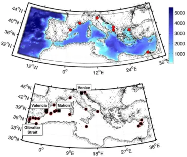
Figure 1.Upper panel: model domain. Bold dashed lines in the At-lantic indicate the location of the lateral boundaries of the model. Red circles indicate river locations and Dardanelles inflow. Bottom panel: black circles indicate tide gauge positions. Dark squares indi-cate the positions of the tide gauges collecting high-frequency data. The Gibraltar Strait is also shown.
In this study, NEMO-MFS-1 is based on NEMO 3.4 code version using a filtered free surface with a 1/16◦
horizon-tal regular resolution, and 72 unevenly spaced verticalz
lev-els with partial cells to fit the bottom depth shape. NEMO-MFS-1 covers the entire Mediterranean Sea and also ex-tends into the Atlantic (Fig. 1, upper panel). The model is forced by momentum, water and heat fluxes interac-tively computed by bulk formulae (Oddo et al., 2009) us-ing the 6 h, 0.5◦ horizontal-resolution operational analyses from the European Centre for Medium-Range Weather Fore-casts (ECMWF) and model-predicted surface temperatures. The ECMWF fields are linearly interpolated onto the model time-step. Atmospheric pressure effects are not included in the model forcings. The natural surface boundary condition for vertical velocity is used.
Only seven major rivers were implemented (Fig. 1, up-per panel): the Ebro, Nile and Rhone monthly values are from the Global Runoff Data Centre (Fekete et al., 1999), the Adriatic rivers Po, Vjose and Seman are from Raicich (Raicich, 1996), while the Bojana River climatological flow is taken from UNEP (1996). The Dardanelles inflow was pa-rameterized as a river and its monthly climatological net in-flow rates and salinity values were taken from Kourafalou and Barbopoulos (2003).
Gibral-Table 1.NEMO–MFS configurations with corresponding cpp keys and namelist variables.
NEMO
MFS-1 MFS-2 MFS-3 MFS-4
Horiz. resolution 1/16 Degree
Vertical discretization 72 z levels with partial cells. (ln_zps=.true.) Horiz. viscosity Bi-LaplacianAmh=5e.9 m4s−1(ln_dynldf_bilap=.true.) Horiz. diffusivity Bi-LaplacianAth= −3.e9 m4s−1(ln_traldf_bilap=.true.) Vertical visc. scheme Pacanowski and Philander (key_zdfric)
Free-surface formulation Filtered (key_dynspg_flt)
Time splitting (key_dynspg_ts)
Time-step 600 s Number of barotropic sub-time stepsnn_baro=100 Initial condition MedAtlas climatology
Air–sea fluxes MFS-bulk formulae (ln_blk_mfs=.true.)
Atmospheric press. No Yes No Yes
ln_apr_dyn= .false. .true. .false. .true.
Runoff As surface boundary condition forSandw(ln_rnf=.true.) Solar radiation 2 Bands penetration (ln_qsr_2bd=.true.)
Lateral momentum B.C. No-sleep
(rn_shlat=2.) Bottom momentum B.C Non linear friction
(nn_bfr=2)
EOS UNESCO – Jackett and McDougall (1995)(nn_eos=0) Tracer advection Up-stream/MUSCL (ln_traadv_muscl=.true.) Momentum advection Vector form (energy and enstrophy cons. scheme)
(ln_dynadv_vec=.true. ln_dynvor_een=.true.) Back. vertical visc. Amv=1.2e−5 m2s−1
Back. vertical diff. Atv=1.2e−6 m2s−1 Vertical visc./diff. scheme Implicit (ln_zdfexp=.false.)
tar, the up-stream scheme, together with an artificially in-creased vertical diffusivity, parameterizes the mixing that acts in this area due to the internal wave breaking, which is not explicitly resolved by the model.
In NEMO-MFS-1, the Atlantic box is nested within the monthly mean climatological fields computed from the daily output of the 1/4◦ global model (Drévillon et al., 2008),
spanning from 2001 to 2005. The two-dimensional adap-tive radiation condition (Marchesiello et al., 2001; Oddo and Pinardi, 2008) was used for the active tracers (temperature and salinity). Total velocities at the open boundaries are im-posed by the global model solution, while barotropic veloci-ties use a modified Flather (1976) lateral boundary condition explained by Oddo and Pinardi (2008). A summary of the model configuration is provided in Table 1, while details on the lateral open boundaries conditions are provided by Oddo et al. (2009).
Three additional NEMO configurations were created for this study. NEMO-MFS-2 is identical to NEMO-MFS-1 ex-cept for the inclusion of the atmospheric pressure forcing. This forcing, like the other atmospheric fields, is taken from ECMWF operational products. NEMO-MFS-3 uses the time-splitting approach to solve the free surface elevation ten-dency Eq. (2), without considering the atmospheric pressure. Finally NEMO-MFS-4 uses the time-splitting method and
also takes account of the atmospheric pressure effects. The differences between the four model configurations are listed in Table 1 while Appendix A provides details on how to re-produce the physical set-up used in this manuscript starting from the standard NEMO code.
All the simulations have been initialized with climato-logical temperature and salinity fields (SeaDataNet, www. seadatanet.org) on 7 January 2004 and ended on 31 Decem-ber 2012.
4 Results and discussion
In this section the sensitivity of the circulation response due to the atmospheric pressure effect is analysed as a function of the free surface elevation formulation in NEMO. Only the different solutions forηare considered since vertical profiles
of temperature and salinity were not found to be significantly different among the four experiments. All the model configu-rations have very similar baroclinic capabilities to each other and to the ones obtained with similar NEMO experiments (Oddo et al., 2009).
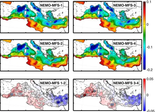
Figure 2.Horizontal maps of the 2-year mean component of the sea surface elevation in the four experiments (units are metres). The two bottom panels represent the sea surface elevation differences between the experiments with and without atmospheric pressure forcing for the time-splitting (right) and the filtered free surface (left) cases.
gauges in the Mediterranean Sea were used (Fig. 1, bottom panel).
Since the Mediterranean’s response to atmospheric pres-sure forcing varies according to the timescales considered (Garret and Majaess, 1984; Lascaratos and Gaˇci´c, 1990), model results are analysed and discussed on the basis of dif-ferent temporal scales. Firstly the low-frequency response re-sults are discussed in terms of model-to-model and models-to-observations comparisons in a period range spanning from the time-invariant components of theηsignal up to 5 days.
The high-frequency model results are then analysed in a pe-riod window from 5 days to 12 h.
4.1 Low-frequency components
The 2-year mean component of the sea surface height (SSH) in the four experiments is shown in Fig. 2. At climatolog-ical timescales there are no significant differences between the twoηnumerical formulations; however, qualitative
dif-ferences in the circulation due to the introduction of pres-sure forcing are evident. The major Mediterranean circula-tion structures (Pinardi et al., 2013) are very similar among the various numerical model formulations but different due to the introduction of atmospheric pressure forcing. This forc-ing generally weakens all the cyclonic wind-driven structures as the atmospheric pressure forces η in the opposite way
from the wind stress curl, i.e. the wind strengthens the cy-clonic structures, whereas the associated atmospheric
pres-sure weakens them. The Adriatic and the Rhode cyclonic gyre circulations illustrate the atmospheric pressure effects well, and the structures are more realistic and closer to re-cent Mediterranean circulation reanalysis studies (Pinardi et al., 2013) in the atmospheric forcing cases.
The maps showing differences between the experiments with and without atmospheric pressure are also similar. A large-scale zonal gradient in the free surface is observed due to atmospheric pressure which produces higherη
val-ues in the Levantine basin and lowerηvalues in the western
Mediterranean Sea. Similar standard deviations maps (not shown) also indicate that, when atmospheric pressure is in-troduced, the Levantine basin has larger seasonal oscillations than the remaining part of the Mediterranean Sea. In the vari-ous experiments, small-scale differences, i.e. eddy-like struc-tures, were observed. These structures have horizontal scales that are much smaller than the atmospheric pressure scales and are probably due to the displacements of oceanic fea-tures as a consequence of instabilities induced by the new forcing.
A comparison between the time-series of daily values of
ηfor the four experiments and corresponding observed data
are shown in Fig. 3. Prior to the comparison, the steric ef-fect was superimposed on the η model outputs, following
Figure 3.Top panel: Mediterranean mean sea-level time-series from the four experiments and observations averaged over the tide gauge positions shown in Fig. 1. The black line represents observational data, the red line represents NEMO-MFS-1 results, the blue line represents NEMO-MFS-2 results, the yellow line represents NEMO-MFS-3 results, and the green line represents NEMO-MFS-4 results. Left middle panel:ηpower spectra for observations and model results, units are cm2. Right middle, left bottom and right bottom panels: coherence, phase (degrees) and gain computed between observations and model, respectively. Units in thexaxis are periods in days.
power spectra comparison and coherency analysis with ob-servations. For the coherency analysis smoothing was per-formed over eight adjacent frequencies. Model results were first interpolated into the tide-gauge positions (Fig. 1, bot-tom panel) and then averaged. In order to evaluate potential sampling errors deriving from the relatively short time inter-val analysed and statistical robustness of the model results, a preliminary spectral analysis has been carried out consid-ering the entire model runs period. In terms of the energetic content and differences between the different model config-urations, no significant differences have been observed be-tween the two time periods considered. Results are shown for periods between 360 and 5 days. However, results for periods shorter than 15 days were shown to be sensitive to specific sampling positions and/or tide gauge locations (in agreement with Garret and Majaess, 1984; Lascaratos and Gaˇci´c, 1990). On the other hand, the modelled response to the atmospheric pressure in the period band between 360 and 15 days was shown to be geographically coherent within the Mediterranean basin.
In agreement with Molcard et al. (2002) and Oddo et al. (2009) and irrespective of the experiment considered, both observational and modelled data are characterized by a large seasonal cycle modulated by inter-annual variability (the inter-annual variability is not shown, since only a 2-year interval series was selected from the model results in order to be consistent with the observational data set available). Qual-itatively, the longer timescales of the inter-annual variability have larger amplitudes in the winter than in the summer. At very low frequencies the major difference in the results de-riving from the two free surface methods is the amplitude of
the seasonal cycle, i.e. the filtered formulation has a larger amplitude.
Comparing the power spectra (Fig. 3, left-middle panel), it is evident that the filtered formulation overestimates the energy content in the spectral window between 360 and 120/100 days. The introduction of the atmospheric pressure slightly reduces this model behaviour (Fig. 3, right-bottom panel). For shorter periods, between 120 and 5 days, the fil-tered formulation generally underestimates the energy con-tent. Also in this case, when the atmospheric pressure in the filtered formulation was introduced, there was a considerable improvement in the reproduction of the energy content.
Overall, the two experiments with the time-splitting for-mulation improved the reproduction of the observed energy content. At seasonal scales, the energy content is consid-erably lower than the filtered simulations and is closer to the observation. However in the window between 180 and 30 days, NEMO-MFS-3 significantly underestimated the ob-served variability due to the missing contribution of atmo-spheric pressure in this period range.
At frequencies between 100 and 5 days−1 NEMO-MFS-3 and NEMO-MFS-1 without atmospheric pressure forcing have very similar energy contents and both underestimated the observed values.
As for the filtered formulation, with the introduction of the atmospheric pressure in the time-splitting experiments, the energy content ofηincreases in the spectral window between
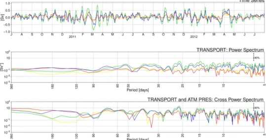
pe-Figure 4.Top panel: Gibraltar transport time-series from the four experiments. Middle panel: Gibraltar transport power spectra. Bottom panel: cross power spectrum between Gibraltar transport and atmospheric pressure. NEMO-MFS1, red; NEMO-MFS2, blue; NEMO-MFS3, yellow; NEMO-MFS4, green.
riods longer than 120/100 days, the numerical scheme used to solve Eq. (2) plays a major role in determining the ocean dynamic (irrespective of the additional forcing introduced), while for periods shorter than 120/100 days, the effect of at-mospheric pressure dominates over the effect of the specific numerical solution method forη.
In all the experiments, the coherence is fairly high (Fig. 3, right-middle panel). There were significant improvements with the introduction of the atmospheric pressure, irrespec-tive of the numerical solution methods, for periods shorter than 50 days. The phase difference is always small and gen-erally below 30◦. There was a significant phase shift between observations and model simulation values between 40 and 25 days in the absence of atmospheric pressure forcing. For periods shorter than 180 days, all the gains are generally smaller than 1, which means that the model underestimated the amplitude ofηoscillations. However there was a
signifi-cant improvement with introduction of the atmospheric pres-sure forcing for periods shorter than 90 days.
The analysis so far was performed for the model and ob-served average sea level at the 25 tide gauge stations (Fig. 1). This can be considered a good estimate of the mean sea level of the Mediterranean Sea for periods between 360 and 15 days because no significant differences were observed at these timescales, averaging over the whole Mediterranean Sea or by only sampling at tide gauge locations.
To elucidate the observed differences between the results of the four experiments in terms of these basin averaged os-cillations, Fig. 4 shows the time-series of net transport at the Gibraltar Strait together with the corresponding power and cross power (with atmospheric pressure) spectra. The mean net transport in the four experiments does not vary significantly, i.e. the time averages are all about 0.05 Sv (in
agreement with previously modelled and observed findings; Oddo et al., 2009). On the other hand, in agreement with La-combe (1961), introducing the atmospheric pressure led to a significant increase in the amplitude of the transport oscilla-tions for periods shorter than 100 days. Furthermore, impor-tant sub-inertial variability in the period band of 10–5 days is observed, while annual or semi-annual signals have small amplitudes, confirming previous studies’ results (Lafuente et al., 2002).
For periods longer than 270 days, introducing the atmo-spheric pressure dampens the amplitude of the transport whichever numerical formulation is used for the free surface elevation, but this effect was larger using the filtered scheme (Fig. 4, middle panel). In the range of 270 and 120 days, the NEMO-MFS-1 and NEMO-MFS-2 simulated transport had a larger energy content than the corresponding NEMO-MFS-3 and NEMO-MFS-4. Between 70 and 30 days, the introduc-tion of atmospheric pressure produced a similar increase in energy content in both the configurations (filtered and time-splitting formulations).
For periods shorter than 25 days, there were clearer differ-ences in atmospheric pressure effect in the two formulations. In these spectral windows, the oscillation in the Gibraltar transport was totally due to the atmospheric pressure-induced dynamics. Peaks in the spectra and in the cross power spectra simulated with the time splitting match peaks simulated us-ing the filtered formulations. However, usus-ing time splittus-ing, the energy content doubled, meaning that the atmospheric pressure effect in the Gibraltar Straits must occur in the form of fast processes filtered out using the filtered formulations.
en-Figure 5.Top panel: phase analysis between Gibraltar transport and surface mass fluxes. Middle panel: Gibraltar transport for the four experiments and surface mass flux reconstructed using only seasonal frequencies. The black line indicates the surface mass fluxes (identical in all the model simulations). Bottom panel: sea’s surface height stochastic component for the four experiments reconstructed using only seasonal frequencies. NEMO-MFS1, red; NEMO-MFS2, blue; NEMO-MFS3, yellow; NEMO-MFS4, green.
ergy content of the Gibraltar transport. Similarly to Pinardi et al. (2014), by integrating Eq. (2) into time and into a semi-enclosed basin such as the Mediterranean Sea, we obtain an equation for the mean sea level tendency:
∂hηi
∂t =
Gib_tr
A − hqw,i (5)
where Gib_tr is the integral of the mass divergence D in
Eq. (3) resulting in the net transport at Gibraltar, A is the
Mediterranean Sea area, and qw is the basin average of the surface mass fluxes, which is identical (not shown) in the four simulations. What modulates the mean sea surface elevation seasonal oscillation differently in the four experiments is the phase shift between the two terms on the right-hand side of Eq. (5). Pinardi et al. (2014) call this difference the stochastic component of the sea surface elevation tendency.
In Fig. 5 (top panel) the phases between the Gibraltar net transport and the surface mass flux (qw) for the four experi-ments are shown. The main differences derive from the intro-duction of the time-splitting scheme, while the atmospheric pressure plays a minor role in modulating the phase of the two signals at seasonal timescales. At higher frequencies (pe-riods shorter than 100 days) the atmospheric pressure effect dominates. In the middle panel of Fig. 5, the Gib_tr and qw reconstructed signals considering only the seasonal frequen-cies are shown; the corresponding stochastic sea surface el-evation component is shown in the bottom panel. Only one time-series of qw is drawn since no significant differences among the experiments are observed. The amplitude of the Gibraltar net transport annual cycle is very similar in all the considered model experiments and its value is about 0.07 Sv; the qw seasonal cycle has an amplitude of about 0.06 Sv. Both Gib_tr and qw modelled seasonal oscillations are in
agreement with previous studies (Lafuente et al., 2002). The phase shift produced using the time-splitting scheme ampli-fies the phase difference between qw and Gib_tr (from 120 to 150 degrees), and the resulting stochastic component has a smaller amplitude. This could have a profound influence on the long-term trend in the sea level in the Mediterranean, as explained by Pinardi et al. (2014).
4.2 High-frequency components
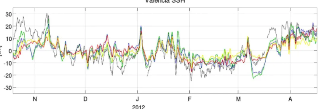
Figure 6. Valenciaηtime-series from observations and model results. Data and model results have been filtered with 5 h running mean. Observations, black; NEMO-MFS1, red; NEMO-MFS2, blue; NEMO-MFS3, yellow; NEMO-MFS4, green.
Figure 7. Valenciaη power spectra from observations and mod-els results. Observations, black; NEMO-MFS1, red; NEMO-MFS2, blue; NEMO-MFS3, yellow; NEMO-MFS4, green.
steric effect superimposed on model results. Modelled and observed sea-level data time-series were also compared by analysing individual power spectra. Power spectra for the three selected stations are drawn in the period band between 5 days and 12 h, while the simulated and observed energetic contents at very high frequencies (between 12 and 2 h−1)are listed in Table 2.
In Figs. 6 and 7 the sea-level time-series and power spec-tra are shown for the station in Valencia. The observed power spectrum is characterized by two distinct maxima, with 24
and 12 h periods respectively. At relatively low frequen-cies (lower than 48 h−1), the experiments without the atmo-spheric pressure underestimated the amplitude of the oscilla-tions. In the range between 48 and 28 h all the experiments performed in a similar way. Differences between numerical schemes and additional forcing are more evident for periods lower than 28 h. Experiments without the atmospheric pres-sure forcing, NEMO-MFS-1 and NEMO-MFS-3, strongly underestimated the amplitude of the signal. By introduction of the atmospheric pressure, the energetic level increased in both NEMO-MFS-2 and NEMO-MFS-4 and both the simu-lations capture the two observed relative maxima at 24 and 12 h. At 24 h the two numerical formulations produce very similar results, both of which underestimate the observed energetic content. The NEMO-MFS-4 simulated energy is closer to the observed values than the corresponding NEMO-MFS-2 result for higher frequencies (12 h−1).
The remaining part of the energetic spectra (frequencies higher than 12 h−1)is certainly affected by the relatively low frequency of the atmospheric forcing and a physical interpre-tation can be misleading. However, although all the model configurations strongly underestimate the observed energy content, NEMO-MFS-4 reaches energetic levels that are sig-nificantly higher than the other NEMO configurations (Ta-ble 2).
inac-Table 2.Energy content (cm2) in the period bands between 12 and 2 h in the three selected stations.
Obs NEMO-MFS1 NEMO-MFS2 NEMO-MFS3 NEMO-MFS4
Valencia 2400 4 16 5 165
Mahon 1900 1 5 2 20
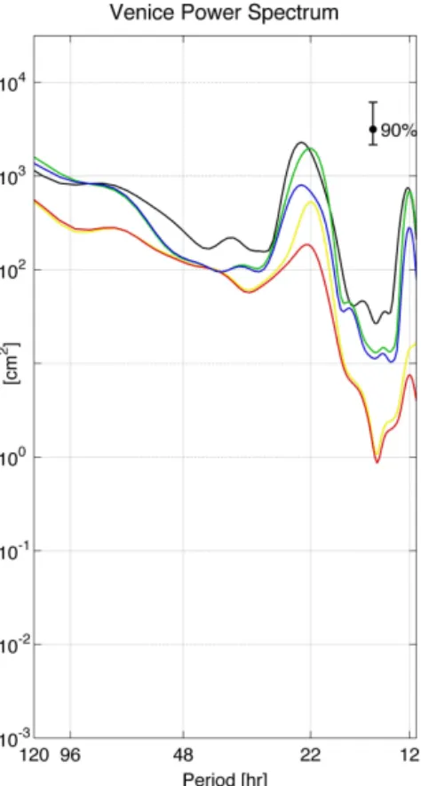
Venice 2500 62 715 190 2400
Figure 8.Mahonη time-series from observations and model results. Data and model results have been filtered with 5 h running mean. Observations, black; NEMO-MFS1, red; NEMO-MFS2, blue; NEMO-MFS3, yellow; NEMO-MFS4, green.
Figure 9.Mahonηpower spectra from observations and model re-sults. Observations, black; NEMO-MFS1, red; NEMO-MFS2, blue; NEMO-MFS3, yellow; NEMO-MFS4, green.
curate representation of the bathymetry. In Mahon, by intro-ducing the atmospheric pressure and using the time-splitting scheme, there was a greater improvement in the represen-tation of the 12 h period maximum although the modelled values remain lower than the observed ones. Theη
formula-tion seems to play a minor role for periods longer than 18 h, while the introduction of the atmospheric pressure forcing was responsible for the differences between the model re-sults. In the spectral windows between 18 and 12 h the en-ergetic levels obtained with the different configurations indi-cate that both additional forcing and the numerical scheme significantly improve the performance of the models. In the period band between 12 and 2 h (Table 2), none of the models managed to reproduce the observed energetic content.
Figure 10. Veniceηtime-series from observations and model results. Data and model results have been filtered with 5 h running mean. Observations, black; NEMO-MFS1, red; NEMO-MFS2, blue; NEMO-MFS3, yellow; NEMO-MFS4, green.
Figure 11.Veniceηpower spectra from observations and model re-sults. Observations, black; NEMO-MFS1, red; NEMO-MFS2, blue; NEMO-MFS3, yellow; NEMO-MFS4, green.
However, the energy content in the time-splitting formula-tion better matches the observed values. Without the atmo-spheric pressure, both the η formulations clearly
underes-timate the amplitude of the free oscillations. The signal is only partially present in the model results (NEMO-MFS-1 and NEMO-MFS-3) due to the wind effect, which is also a driver for the seiches’ dynamic (Leder and Orli´c, 2004). In Venice the model’s sensitivity to atmospheric pressure and
η formulation is significantly different from what was
ob-served in Valencia and Mahon. In the latter two stations the different numerical scheme used to solve Eq. (2) affected the model results only for periods shorter than 18/16 h, while in
Venice differences are evident for 24 h period oscillations. It is interesting to note that in the frequency band between 12 and 2 h−1(Table 2), NEMO-MFS4 reaches and supports energetic levels similar to the observations, while the other models strongly underestimate the amplitude of the signal in this frequency band. A model configuration such as NEMO-MFS4 might be able to correctly resolve the high-frequency dynamic of the Adriatic Sea if forced with adequate atmo-spheric data.
5 Summary and conclusions
The sensitivity of the Mediterranean Sea ocean dynamics to the free surface elevation numerical formulation in NEMO was evaluated for cases with and without atmospheric pres-sure forcings. Four different NEMO configurations were cre-ated and the results compared with each other and with avail-able observations. All the NEMO configurations were imple-mented using the same horizontal and vertical meshes.
The reference NEMO configuration, NEMO-MFS-1, uses a filtered formulation of the free surface equation (Roullet and Madec, 2000) and does not take account of the atmo-spheric pressure effects. This model set-up is currently used in the framework of the MFS (Pinardi and Flemmings, 1989). NEMO-MFS-2 differs from NEMO-MFS-1 due to the introduction of the atmospheric pressure forcing. The free surface equation is solved using a time-splitting approach (Griffies, 2004) which either does or does not account for the atmospheric pressure effect in MFS-3 and NEMO-MFS-4 configurations, respectively.
values in the east and lower in the west) and a weakening of all the cyclonic wind-driven structures irrespective of the free surface formulation adopted. The structure of the sea level and the corresponding circulation could be considered more realistic with atmospheric pressure forcing, although obser-vational evidence is lacking at the basin scale.
At low frequencies, the major difference between the two numerical free surface formulations is the amplitude of the seasonal cycle. The filtered formulation overestimated the energy content in the spectral window between 400 and 120 days. The amplitude of the seasonal cycle in the time-splitting NEMO formulation was considerably smaller than in the filtered simulations and was closer to the observations. The introduction of atmospheric pressure slightly improved the filtered solution, but did not influence the time-splitting simulation results. With shorter periods (between 120 and 50 days), the simulations without the atmospheric pressure forcing generally underestimated the energy content.
For periods longer than 120/100 days, differences in the
model numerical schemes led to quantitative differences in the sea level (irrespective of the atmospheric pressure), while for shorter periods, atmospheric pressure effects dominated.
In the analysed frequency windows, the time-splitting and filtered formulation responses to the introduction of atmo-spheric pressure were very similar; higher energy levels were reached with the time-splitting scheme and atmospheric pres-sure for short periods.
The mean net transport at the Gibraltar Strait in the four experiments did not vary significantly. At seasonal timescales, the introduction of the atmospheric pressure dampened the amplitude of the net transport in both the free surface numerical formulations. This effect was greater using the filtered scheme. In the periods longer than and 120 days, the NEMO-MFS-1 and NEMO-MFS-2 simulated transport had a larger energy content than the corresponding NEMO-MFS-3 and NEMO-MFS-4 values. In addition, with the in-troduction of the atmospheric pressure, there was a signif-icant increase in the amplitude of the transport oscillations for periods between 70 and 30 days.
At higher frequencies, the differences in the atmospheric pressure effect in the two sea-level formulations are more ev-ident. In these spectral windows, the oscillation in the Gibral-tar transport was totally due to the atmospheric pressure in-duced dynamics. With the use of time splitting, the energy content doubled.
An interesting finding of this study is the effect of the nu-merical scheme on the phase shift between Gibraltar trans-port and surface mass fluxes. This phase shift modulated theηseasonal oscillation differently in the four experiments.
The main differences in the four experiments derive from the introduction of the time-splitting formulation, while atmo-spheric pressure forcing plays a minor role in modulating the phase of the two signals at seasonal scales. The phase shift produced using time splitting amplifies the phase opposition between surface mass fluxes and the Gibraltar transport, and the resulting stochastic component of the sea-level tendency has a smaller amplitude.
An analysis of the observed and modelled high frequencies data sets in three different locations in the Mediterranean Sea (although two locations are relatively close to each other: Va-lencia and Mahon) highlights that the interaction between at-mospheric pressure and barotropic dynamics follows differ-ent dynamics. In Mahon, an open ocean station in the western Mediterranean Sea (Fig. 1, bottom panel), the introduction of the atmospheric pressure forcing in the model improves the reproduction of the observedηvariability and energetic
con-tent in the spectral window between 20 and 12 h. In Valencia, the additional pressure forcing affects the results of the model also for oscillations with 24 h period. On the other hand, in both stations the introduction of the atmospheric pressure al-lows the model to reach energetic levels similar to the obser-vation for periods longer than 48 h. In Venice, located in the northernmost part of a semi-enclosed basin and characterized by very shallow water, the introduction of the atmospheric pressure clearly improved the model’s capability to correctly simulate the seiches, which, in addition to wind regimes, are driven by the atmospheric pressure differences between the north and south Adriatic. However, it is the explicit resolu-tion of the barotropic processes (using the time splitting) that allows the model to correctly simulate theηdynamics at high
Appendix A
The NEMO model is freely available under the CeCILL public licence. After registering at the NEMO website (http://www.nemo-ocean.eu), users should follow the proce-dure described in the “NEMO Quick Start Guide” section to access and run the model. The physical set-up of the config-urations used in the present paper can be obtained starting from the GYRE standard configuration and modifying the following parameters.
– CPP keys: – GYRE:
– key_gyre key_dynspg_flt key_ldfslp key_zdftke key_iomput
– NEMO-MFS-3andNEMO-MFS-4:
– key_myconfig key_mpp_mpi key_obc key_zdfric key_dynspg_ts key_iomput
– NEMO-MFS-1andNEMO-MFS-2:
– key_myconfig key_mpp_mpi key_obc key_zdfric key_dynspg_flt key_iomput
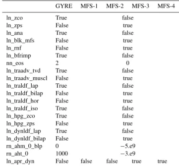
Namelist values should be modified according to Ta-ble A1.
Table A1.Namelist.
GYRE MFS-1 MFS-2 MFS-3 MFS-4
ln_zco True false ln_zps False true ln_ana True false ln_blk_mfs False true ln_rnf False true ln_bfrimp True false
nn_eos 2 0
ln_traadv_tvd True false ln_traadv_muscl False true ln_traldf_lap True false ln_traldf_bilap False true ln_traldf_hor False true ln_traldf_iso True false ln_hpg_zco True false ln_hpg_zps False true ln_dynldf_lap True false ln_dynldf_bilap False true rn_ahm_0_blp 0 −5.e9 rn_aht_0 1000 −3.e9
Acknowledgements. This work was supported by the European Commission MyOcean 2 Project (FP7-SPACE-2011-1-Prototype Operational Continuity for the GMES Ocean Monitoring and Forecasting Service, GA 283367) and by the Italian Project RITMARE, la RIcerca iTaliana per il MARE (MIUR-Progetto Bandiera 2012–2016).
Edited by: A. Yool
References
Candela, J. and Lozano C. J.: Barotropic response of the west-ern Mediterranean to observed atmospheric pressure forc-ing, in: Seasonal and Interannual Variability of the Western Mediterranean Sea, Coastal Estuarine Stud., vol. 46, edited by: La Viollette, P. E., 325–359, AGU, Washington, D. C., doi:10.1029/CE046p0325, 1994.
Cerovecki, I., Orli´c, M., and Hendershott, M. C.: Aadriatic seiche decay and energy loss to the Mediterranean, Deep-sea research. Part 1. Oceanographic research papers, 44, 2007–2029, 1997. Crépon, M.: Influence de la pression atmosphérique sur le niveau
moyen de la Méditerranée Occidentale et sur le flux à travers le détroit de Gibraltar, Cah. Océanogr., 17, 15–32, 1965.
Demirov, E. and Pinardi, N.: The simulation of the Mediterranean Sea circulation from 1979 to 1993, Part I: The interannual vari-ability, J. Mar. Syst., 33–34, 23–50, 2002.
Drévillon, M., Bourdallé-Badie, R., Derval, C., Drillet, Y., Lel-louche, J. M., Rémy, E., Tranchant, B., Benkiran, M., Greiner,E., Guinehut, S., Verbrugge, N., Garric, G., Testut, C. E., Laborie, M., Nouel, L., Bahurel, P., Bricaud, C., Crosnier, L.,Dombrosky, E., Durand, E., Ferry, N., Hernandez, F., Le Galloudec, O., Messal, F., and Parent, L.: The GODAE/Mercator-Ocean global ocean forecasting system: results, applications and prospects, J. Operational Oceanogr., 1, 51–57, 2008.
Dukowiz, J. K., Smith, R. D., and Malone, R. C.: A reformulation and implementation of the Bryan-Cox0Semtner ocean model on the connection machine, J. Atmos. Ocean Technol., 10, 195–208, 1993.
Estubier, A. and Levy, M.: Quel schema numerique pour le trans-port d’organismes biologiques par la circulation oceanique, Note Techniques du Pole de modelisation, Institut Pierre-Simon Laplace, 81 pp., 2000.
Fekete, B. M., Vorosmarty, C. J., and Grabs, W.: Global, compos-ite runoff fields based on observed river discharge and simulated water balances, Tech. Rep. 22, Global Runoff Data 25 Cent., Koblenz, Germany, 1999.
Flather, R. A.: A tidal model of the northwest European continental shelf, Memories de la Societe Royale des Sciences de Liege, 6, 141–164, 1976.
Garrett, C. J. R.: Variable sea level and strait flows in the Mediter-ranean: A theoretical study of the response to meteorological forcing, Oceanol. Acta, 6, 79–87, 1983.
Garrett, C. J. R. and Majaess, F.: Nonisostatic response of sea level to atmospheric pressure in the Eastern Mediterranean, J. Phys. Oceanogr., 14, 656–665, 1984.
Godin, G. and Trotti, L.: Trieste-water levels 1952–1971: A study of the tide, mean level and 20 seiche activity, Environment Canado, Fisheries and Marina Services, Miscellaneous Special
Publica-tion, Dept. of the Environment, Fisheries and Marine Service in Ottawa, 28, 1975.
Gomis, D., Tsimplis, M. N., Martín-Míguez, B., Ratsimandresy, A. W., García-Lafuente, J., and Josey, S. A.: Mediterranean Sea level and barotropic flow through the Strait of Gibraltar for the period 1958–2001 and reconstructed since 1659, J. Geophys. Res., 111, C11005, doi:10.1029/2005JC003186, 2006.
Gomis, D., Ruiz, S., Sotillo, M. G., Álvarez-Fanjul, E., Terradas, J.: Low frequency Mediterranean sea level variability: The contri-bution of atmospheric pressure and wind, Global Planet Change, 63, 215–229, 2008.
Griffies, S. M.: Fundamentals of ocean climate models, Princeton University Press, 434 pp., 2004.
Jackett, D. R. and McDougall, T. J.: Minimal Adjustment of Hy-drostatic Profiles to Achieve Static Stability, J. Atmos. Ocean. Technol., 12, 381–389, 1995.
Kasumovi´c, M.: On the influence of air pressure and wind on the Adriatic Sea level fluctuations, Hidrografski godišnjak, 1956/57, 107–121, 1958 (in Croatian).
Kourafalou, V. H. and Barbopoulos, K.: High resolution simulations on the North Aegean Sea seasonal circulation, Ann. Geophys., 21, 251–265, doi:10.5194/angeo-21-251-2003, 2003.
Lacombe, H.: Contribution à l’étude du détroit de Gibraltar, étu de dynamique, Cah. Océanogr., 12, 73–107, 1961.
Lafuente J. G., Delgado, J., Vargas, J. M., Sarhan, T., Vargas, M., and Plaza, F.: Low frequency variability of the exchanged flows through the Strait of Gibraltar during CANIGO, Deep Sea Res., 49, 4051–4067, 2002.
Lascaratos, A. and Gaˇci´c, M.: Low-Frequency Sea Level Variability in the Northeastern Mediterranean., J. Phys. Oceanogr., 20, 522– 533, 1990.
Leder, N. and Orli´c, M.: Fundamental Adriatic seiche recorded by current meters, Ann. Geophys., 22, 1449–1464, doi:10.5194/angeo-22-1449-2004, 2004.
Le Traon, P. Y. and Gauzelin, P.: Response of the Mediterranean mean sea level to atmospheric pressure forcing, J. Geophys. Res., 102, 973–984, 1997.
Madec, G.: NEMO ocean engine, Note du Pole de modelisa-tion, Institut Pierre-Simon Laplace (IPSL), France, No 27 ISSN No1288-1619, 2008.
Marchesiello, P., McWilliams, J. C., Shchepetkin, A.: Open bound-ary conditions for long term integration of regional oceanic mod-els, Ocean Model., 3, 1–20, 2001.
Marcos, M. and Tsimplis, M. N.: Variations of the seasonal sea level cycle in southern Europe, J. Geophys. Res., 112, C12011, doi:10.1029/2006JC004049, 2007.
Mellor, G. L. and Ezer, T.: Sea level variations induced by heat-ing and coolheat-ing: An evaluation of the boussinesq approximation in ocean models, J. Geophys. Res.-Oceans, 100, 20565–20577, doi:10.1029/95JC02442, 1995.
Molcard, A., Pinardi, N., Iskandarami, M., and Haidvogel, D. B.: Wind driven general circulation of the Mediterranean Sea sim-ulated with a Spectral Element Ocean Model, Dynam. Atmos. Oceans, 17, 687–700, 2002.
Mosetti, F.: Considerazioni sulle cause dell’acqua alta a Venezia, Boll. Geofis. Teor. Appl., 13, 169–184, 1971.
Oddo, P., Adani, M., Pinardi, N., Fratianni, C., Tonani, M., and Pet-tenuzzo, D.: A nested Atlantic-Mediterranean Sea general circu-lation model for operational forecasting, Ocean Sci., 5, 461–473, doi:10.5194/os-5-461-2009, 2009.
Orli´c, M.: On frictionless influence of planetary atmospheric waves on the Adriatic sea level, J. Phys. Oceanogr., 13, 1301–1306, 1983.
Palumbo, A. and Manzzarella, A.: Mean sea level variations and their practical applications, J. Geophys. Res., 87, 4249–4256, 1982.
Papa, L.: A statistical investigation of low-frequency sea level varia-tion at Genoa, Istituto Idrografico della Marina, Universita’ degli strudi di Genova, F.C., 1987, Grog 6, 13 pp., 1978.
Pasaric, M., Pasaric, Z., and Orlic, M.: Response of the Adriatic sea level to the air pressure and wind forcing at low frequencies (0.01–0.1 cpd), J. Geophys. Res., 105, 11423–11439, 2000. Pascual, A., Marcos, M., and Gomis, D.: Comparing the sea level
response to pressure and wind forcing of two barotropic models: Validation with tide gauge and altimetry data. J. Geophys. Res., 113, C07011, doi:10.1029/2007JC004459, 2008.
Pinardi, N. and Flemming, N. C.: The Mediterranean Forecasting System Science Plan, EuroGOOS Publication no. 11, Southamp-ton Oceanography Centre, 48 pp., ISBN 0-904175-35-9, 1998. Pinardi, N., Rosati, A., and Pacanowski, R. C.: The sea surface
pres-sure formulation of rigid lid models. Implications for altimetric data assimilation studies, J. Marine Syst., 6, 109–119, 1995. Pinardi, N., Allen, I., Demirov, E., De Mey, P., Korres, G.,
Las-caratos, A., Le Traon, P.-Y., Maillard, C., Manzella, G., and Tziavos, C.: The Mediterranean ocean forecasting system: first phase of implementation (1998–2001), Ann. Geophys., 21, 3–20, doi:10.5194/angeo-21-3-2003, 2003.
Pinardi, N., Zavatarelli, M., Adani, M., Coppini, G., Fra-tianni, C., Oddo, P., Simoncelli, S., Tonani, M., Lyubart-sev, V. Dobricic, S., Bonaduce, A.: Mediterranean Sea Large-scale low-frequency ocean variability and water mass for-mation rates from 1987 to 2007: A retrospective analysis, doi:10.1016/j.pocean.2013.11.003, 2013.
Pinardi, N., Bonaduce, A., Navarra, A., Dobricic, S., and Oddo, P.: The mean sea level equation and its application to the Mediter-ranean sea, J. Climate, 27, 442–447, doi:10.1175/JCLI-D-13-00139.1, 2014.
Ponte, R. M.: Variability in a homogeneous global ocean forced by barometric pressure, Dyn. Atmos. Oceans, 18, 209–234, 1993. Raicich, F.: On fresh water balance of the Adriatic Sea, J. Marine
Syst., 9, 305–319, 1996.
Raicich, F., Orlîc, M., Vilibîc, I., Malacîc, V., A case study of the Adriatic seiches (December 1997), Il Nuovo Cimento C, 22, 715–726, 1999.
Roullet, G. and Madec, G.: salt conservation, free surface, and vary-ing levels: a new formulation for ocean general circulation mod-els, J. Geophys. Res., 105, 23927–23942, 2000.
UNEP: Implications of Climate Change for the Albanian Coast, Mediterranean Action Plan, MAP Technical Reports Series No. 98., 1996.
Van Leer, B.: Towards the Ultimate Conservative Difference Scheme, V. A Second Order Sequel to Godunov’s Method, J. Comp. Phys., 32, 101–136, 1979.
Wakelin, S. L. and Proctor, R.: The impact of meteorology on mod-elling storm surges in the Adriatic Sea, Global Planet. Change, 34, 97–119, 2002.