Abstract—Nowadays, several positioning systems are available for outdoor localization, such as the global positioning system (GPS), assisted GPS (A-GPS), and other techniques working on cellular networks, for example, Time of Arrival (TOA), Angle of Arrival (AOA) and Time Difference of Arrival (TDOA).However, with the increasing use of mobile computing devices and an expansion of wireless local area networks (WLANs), there is a growing interest in indoor wireless positioning systems based on the WLAN infrastructure. Wireless positioning systems (WPS) based on this infrastructure can be used for outdoor / indoor localization to determine the position of mobile users. An important factor in achieving this is to minimize and simplify the instructions that the mobile station (MS) has to execute in the location determination process. Finding an effective location estimation technique to facilitate processing data is the main focuses in this paper. Therefore, in the wireless propagation environment the Received Signal Strength (RSS) information from three base stations (BSs) are recorded and processed and they can provide an overlapping coverage area of interest. Then an easy new geometric technique is applied in order to effectively calculate the location of the desired MS.
Our new positioning method design was verified at the algorithmic level using Matlab tool, described in Very-high-speed integrated circuit Hardware Description Language (VHDL) at the register transfer level (RTL) and it has been synthesized using 7.1 version of FPGA Advantage for HDL Design that evaluates the circuit in terms of speed, area and power consumption.
Index Terms—Geometric technique, Position estimation, Wireless LAN, VHDL.
I. INTRODUCTION
Recently, the subject of mobile positioning in wireless communication systems has drawn considerable attention. With accurate location estimation, a variety of new applications and services such as Enhanced-911, location sensitive billing, improved fraud detection, intelligent
Monji Zaidi, Jamila Bhar and Rached Tourki are with Electronic and Micro-Electronic Laboratory (EµE, IT-06).FSM, Monastir, Tunisia
Ridha Ouni is with College of Computer and Information Sciences (CCIS), King Saud University Riyadh, KSA
transport system (ITS) and improved traffic management will become feasible [1]. Mobile positioning using radiolocation techniques usually involves time of arrival (TOA), time difference of arrival (TDOA), angle of arrival (AOA), signal strength (SS) measurements or some combination of these methods.
All of these methods are mainly based on trigonometric computation. Comparisons and survey of these methods are given in [2] and [3].
The TOA technique determines the MS position based on the intersection of three circles. Two range measurements provide an ambiguous fix, and three measurements determine a unique position.
Given the coordinates of BSj, (j = 1, 2, 3) as (Xj, Yj), and the distances dj between MS and BSj, the simplest geometrical algorithm for TOA positioning (Figure. 1(a)) is given in [2]. Coordinates of MS position (x,y) relative to BS1 can be calculated as:
=12 + ++ ++ −−
The simplest geometrical algorithm for TDOA positioning (Figure. 1(b)) is given in [4]. There are two estimated TDOA-s dj, 1 between BS1 and the jth base station (j = 2, 3). Coordinates of MS position (x, y) relative to BS1 can be calculated in terms of d1 as:
= − ∗ ,
, +
1
2 ,, −− ++
Where:
= +
= +
= +
The AOA technique determines the MS position (x, y) based on triangulation, as shown in (Figure. 1(c)). The intersection of two directional lines of bearing with angles θ and θ defines a unique position, each formed by a radial from a BS to the MS. The simplest geometric
Monji ZAIDI, Ridha OUNI, Jamila Bhar and Rached TOURKI
A Novel Positioning Technique with Low
Complexity in Wireless LAN:
solution can be derived using [5] with two AOA measurements θ and θ :
x =Y − Y + X tan(θ ) − X tan (θ )tan(θ ) − tan (π − θ )
y = Y + (x − X )tan(θ )
BS1
BS2
BS3
MS
Hyperbola 1 Hyperbola 2 d 1
d 2
d 3
(b)
BS1
BS3
BS2
d 1
d 2
d 3
MS
(a)
BS1 BS2
MS
2
θ
1
θ
(c)
Fig. 1. Position determination techniques: (a) TOA; (b) TDOA; (c) AOA
Using any of the mentioned methods, the calculation can be done either at the BS [network-based schemes] or at the MS [mobile-based schemes]. Network-based schemes have high network cost and low accuracy [3]. Mobile-based location schemes are more interesting. However, since the MS has limited energy source, in the form of the battery pack, energy consumption should be minimized. An important factor in achieving this is to minimize and simplify the instructions that the MS has to execute in the location determination process. The conventional algorithms use complex computation methods that needed relatively long execution time.
In this paper, we propose a novel wireless positioning technique based on the WLAN infrastructure. The main motivation for our approach is twofold: to improve the accuracy of the location estimation and to minimize and simplify the instructions that the mobile station (MS) has to execute in the location determination process.
II. RELATEDWORK
To improve the accuracy of the indoor positioning system, several techniques demonstrate the viability of this approach. Youssef et al. [6] show that the RADAR system can be improved using the perturbation technique (joint clustering technique) to handle the small-scale variations problem. This technique can improve theRADARsystem and provide location accuracy up to 3m.
The triangulation mapping interpolation system (CMU-TMI) [7] performs a location calculation on the current data, interpolates that data with the information in the database, and then returns a location estimate based on this interpolation. However, power consumption increases to measure the signal strength on the client side.
The Ekahau Positioning Engine 4.0 [8], released in October 2006, also uses an IEEE 802.11 network to provide location information. It achieves an average
accuracy of 1m with at least three audible channels in each location. This system requires site calibration up to 1 h per 1,200m2. While calibration-based efforts present good accuracy results, there is still room for performance enhancements. Due to the very dynamic nature of the RF signal, the assumption that the radio map built in the calibration phase remains consistent to the measurements performed in the real-time phase does not hold in practice; thus, at times, there is a need to rebuild the radio map. It seems more reasonable to design a fully-automatic system capable of acknowledging RSSI characteristics and variations in both spatial and time domains.
Hitachi [9] released location technology based on TDOA in March 2005. This system uses two types of access points: a Master AP and a Slave AP. Slave APs synchronize their clocks with that of a Master AP and measure the arrival time from a mobile terminal; the Master AP determines the location of the mobile terminal using the TDOA between the signal reception times at multiple Slave APs. While this technique has been found to achieve good results in indoor environments, it requires specialized hardware and fine-grain time synchronization, which increases the cost of this type of solution.
Kanaan proposed a closest-neighbor with TOA grid algorithm (CN-TOAG) [10]. This geolocation algorithm presents a TDOA-based position detection technique to improve location accuracy in the indoor environment by estimating the location of the user as the grid point. This technique is similar to the previous one [11], as it needs specialized hardware and fine grain time synchronization, which increase costs.
III. NEWGEOMETRICLOCATIONALGORITHM BASEDONTHREEBSS
In the general geometrical triangulation location researches, they assumed that the measured noise is additive and the NLOS error is a large positive bias which causes the measured ranges to be greater than the true ranges [12].
BS1 BS2
BS3
A B
C
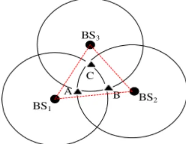
Fig. 2. Measured range circles and the associated intersected area
is necessarily located in the region formed by the points BS1, BS2 and BS3. But, it is noted that the intersection of three circles may not be overlapped with the real measurement results. Therefore, with the above assumption we have to judge whether the three circles intersect or not in our location algorithm.
If circles intersect as depicted in Figure. 3, then three triangles can be drawn as: BS1MSBS2, BS2MSBS3 and BS3MSBS1.
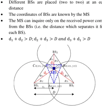
Assumptions:
• Different BSs are placed (two to two) at an equal distance
• The coordinates of BSs are known by the MS
• The MS can inquire only on the received power coming from the BSs (i.e. the distance which separates it from each BS).
• d + d > (; d + d > ( *+ d + d > (
BS1 BS2
BS3
MS
d1 d2
d3
23
θ
21
θ
12
θ
13
θ
32
θ
31
θ
) , (12 12 0x y
A
) , (23 23 0x y
B
) , (31 31 0x y
C
D
r1
Fig. 3. The associated triangles of the standard intersection of three circles.
Note by:
• D: The distance between tow BSs.
• A0, B0 and C0 are the orthogonal projections of the MS on (BS1 BS2), (BS2, BS3) and (BS3 BS1) respectively. • d1, d2 and d3 are the distances that separate the MS
from BS1, BS2 and BS3 respectively.
• θ12: is the geometrical angle between the MS-BS1 and BS1-BS2. (Same things for the other angles).
We focus firstly on the triangle BS1MSBS2.
Based on the above assumptions and figure 2, we can write.
r = d cosθ
We can also write
d = (D − r ) + (d − r ) ⟹
d = (D − d cosθ ) + (d − d cosθ ) ⟹
d = D + d − 2Dd cosθ = D + d − 2Dr ⟹
r =D + d − d2D
We define here the first factor q by
q =rD =D + d − d2D
Coordinates (x , y ) of the point A0 are given in [13] by
x = q X + (1 − q )X y = q Y + (1 − q )Y
Where:
(X , Y ) and (X , Y ) are the coordinates of BS1 and BS2, respectively.
Let the distance between BS2 and B0 be r and the distance between BS3 and C0 be r
As we described previously, we can get the coordinates of points B0 and C0 as:
x = q X + (1 − q )X y = q Y + (1 − q )Y x = q X + (1 − q )X y = q Y + (1 − q )Y
Where:
q =rD =D + d − d2D
q =rD =D + d − d2D
MS is then located in a new triangle A0B0C0, which is smaller in terms of area compared to the starting triangle BS1BS2BS3. In the other word we have just created three
new virtual BSs placed at A0, B0 and C0.
It is very easy to calculate the distances between the MS and the new points A0, B0 and C0 using the Pythagoras formula. Thus
d(MS, A6) = 7d − r
d(MS, B6) = 7d − r
d(MS, C6) = 7d − r
After a small number of iterations, the coordinates of three vertices of the triangle (A, B and C) converge to the actual coordinates of the MS. At the limit, the triangle AconvBconvCconv with vertices Aconv, Bconv and Cconv will be considered as a point. So, it is possible to write:
x=>?@A ≈ xC>?@A≈ xD>?@A
y=>?@A≈ yC>?@A≈ yD>?@A
We can then take the coordinates of the MS as:
xEF=x=>?@A+ xC>?@A3 + xD>?@A
yEF=y=>?@A+ yC>?@A3 + yD>?@A
The division by 3 implies that the MS is equivalent to the gravity center of the Aconv, Bconv Cconv triangle.
Figure 8 (section 5) shows the evolution and the convergence of the three vertices coordinates for different values of di (d1, d2 and d3).
IV. VHDLMODEL
The operation destined to calculate the coordinates of a mobile terminal is known as a Location Process. Original design of this process, has just considered.
Figure 4 shows the main elements involved in our new mechanism: the MS, Three BSs, and the distribution system (DS) or Ethernet.
It can mentioned that different BSs are placed (Two to two) at an equal distance, and the MS can inquire only on the position and the received time coming from the BSs (i.e. the distance which separates it from each BS)
The equations for the x and y position of the mobile was modeled using VHDL. The numeric_std package was used to construct the VHDL model that was readily synthesized into a low power digital circuit. The input signal of the model are the x, y positions of the three BSs, i,j,k in meters, and the signals TOA from the individual BS to the mobile in nanoseconds. The input signal assignments are xi, yi, TOAi, xj, yj, TOAj, xk, yk, TOAk
Fig. 4. Involved elements in the Positioning process
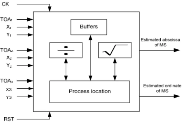
Now, we describe the hardware implementation of the location process. Figure 5 illustrates the system architecture; we try to divide location process to 4 parts: a process location algorithm, the square root component, divider block and buffers to store data. The following notations are used to describe the signal type: I: input signal; O: output signal
TABLE I
PROCESS LOCATION PART INTERFACE SIGNALS
Name Type Description
CK I:bit Operation clock.
RST I:bit RESET system
TOA1 I:std_logic_vector Input from the BS1, it gives the time of arrival value to travel the d1distance X1 I:std_logic_vector BS1 abscissa
Y1 I:std_logic_vector BS1ordinate
TOA2 I:std_logic_vector Input from the BS2, it gives the time of arrival value to travel the d2 distance. X2 I:std_logic_vector BS2 abscissa
Y2 I:std_logic_vector BS2abscissa
TOA2 I:std_logic_vector Input from the BS3, it gives the time of arrival value to travel the d3 distance. X3 I:std_logic_vector BS3 abscissa
Y3 I:std_logic_vector BS3 abscissa
Xestim O:
std_logic_vector
Estimated abscissa of MS
Yestim O:
std_logic_vector
Estimated ordinate of MS
First, the main program (process location) receives data from the external environment. Then, it calculates the parameters r , q , r , q , r , and q as it was presented in Section 3. During this stage the divider component is called by the main program to perform the operations division.
Meanwhile the virtual coordinates
(x , y ), (x , y ) and (x , y ) of points A0, B0 and C0 respectively, are determined.
Secondly, the distances d(MS, A6), d(MS, B6) and
d(MS, C6) are calculated using the square root operators
Fig. 5. Top level structure of the Location circuit
numbers in FPGA arithmetic. Operations on unsigned integers are often simpler to implement, and they require less chip area and resources. The square root operator assumes that its input argument has already been converted into an unsigned integer, which must be taken care of if an application uses signed integers.
A symbol of the top-level VHDL design entity of the square root operator with parameterizable input argument width is presented in Figure 6.
Fig. 6. Top level diagram of the square root operator
Figure 7 shows the simulation of a fast Location processing model. Optimal process latency is improved by reducing the iterations number needed for convergence. So, after a small number of iterations, the coordinates of three vertices of the triangle (A, B and C) converge to the actual coordinates of the MS. at this time, the triangle AconvBconvCconv with vertices Aconv, Bconv and Cconv will be considered as a point and we can write:
x=>?@A = xC>?@A= xD>?@A
y=>?@A= yC>?@A= yD>?@A
We can then take the coordinates of the MS as:
(xEF=HIJKLMNHOJKLMNHPJKLM , yEF=QIJKLMNQOJKLMNQPJKLM)
The division by 3 implies that the MS is equivalent to the gravity center of the AconvBconvCconv triangle.
The (xEF, yEF) Geolocalisation information, obtained with a minimal cost has a very important role in several applications. We are trying to take advantage of this important information to develop a fast handover in an environment with time constraints
Fig. 7. Simulation results of the hardware positioning process
Now, it is necessary, as in any positioning method, to evaluate the error or deviation (in m) between actual (measured) and simulated values obtained by our method. For this two cases have to be considered:
A. Line-of-sight (LOS) condition
This case occurs in open areas or in very specific spots in city centers, in places such as crossroads or large squares with a good visibility of BS. Sometimes, there might not be a direct LOS signal but a strong specular reflection off a smooth surface such as that of a large building will give rise to similar conditions. The received signal will be strong and with moderate fluctuations. Therefore, the extracted distance from the received signal is correctly calculated.
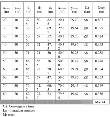
In the table 1 we give some actual locations of the MS (Actual x and y). Corresponding values of the true distances d1, d2 and d3 which separate it from BS1, BS2 and BS3 are calculated. Then the estimated position and position error can be determined using our geometric method.
A. Non Line-of-sight (NLOS) condition
This case will typically be found in Indoor environments. This is a worst-case scenario since the direct signal is completely blocked out and the overall received signal is only due to multipath, thus being weaker and subjected to marked variations. Under these conditions the geometric method can be applied. However, the position error increases significantly.
Fig. 8. Algorithm convergence with (d1, d2, d3) = (52 m, 76 m, 50 m)
The oboe simulation was done with the following BSs coordinates.
BS1 coordinates (in meters):(X , Y ) = (0,0) BS2 coordinates (in meters):(X , Y ) = (100,0) BS3 coordinates (in meters):(X , Y ) = (50,86)
0 5 10 15 20 30
40 50 60
x(A)variations as function of iterations number
iterations number
x
(A
)
0 5 10 15 20 20
40 60 80
x(B)variations as function of iterations number
iterations number
x
(B
)
0 5 10 15 20 25
30 35 40
x(C)variations as function of iterations number
iterations numbers
x
(C
)
0 5 10 15 20 0
20 40 60
y(A)variations as function of iterations number
iterations numbers
y
(A
)
0 5 10 15 20 30
40 50 60
y(B)variations as function of iterations number
iterations number
y
(B
)
0 5 10 15 20 30
35 40 45
y(C)variations as function of iterations number
iterations number
y
(C
)
0 5 10 15 20 30
35 40
45 estimated abscissa of MS
iterations number
x
(M
S
)
0 5 10 15 20 30
35
40 estimated ordinate of MS
iterations number
y
(M
S
TABLE II
LOS MEASUREMENT AND POSITION DETERMINATION
xactua (m) yactua (m) d1 (m) d2 (m) d3 (m) xestima (m) yestima (m) C.t (i.n) Error (m)
20 10 22.
5 80. 5 82. 5 20.1 3
09.20 ≤8 0.807
30 20 36 73 69.
5 29.8 3
19.64 ≤8 0.395
40 30 50.
5
67 57. 5
40.3 0
29.70 ≤8 0.424
40 40 57 72 47.
5 40.3 2
39.86 ≤8 0.353
50 50 71 71 36 50.0
0
50.23 ≤8 0.238
50 70 86.
5 86. 5
16 50.0 0
70.47 ≤8 0.478
60 60 85.
2
72 28. 5
60.3 7
59.91 ≤8 0.384
60 40 72 57 47.
5 59.6 7
39.86 ≤8 0.353
70 30 76.
5 42. 5 60. 5 70.0 6
29.45 ≤8 0.549
80 20 82.
5 27. 9
73 79.8 5
19.69 ≤8 0.336
M≈0.4 C.t: Convergence time
I.n = Iterations number M: mean
TABLE III
NLOS MEASUREMENT AND POSITION DETERMINATION
xactual (m) yactual (m) xestimated (m) yestimated (m) Error (m)
20 10 18.9700 8.4826 1.8340
30 20 29.0950 19.2922 1.1489
40 30 39.0763 28.7347 1.5666
40 40 41.4850 40.8110 1.6920
50 50 50.0000 51.0523 1.0523
50 70 48.2600 70.9884 2.0011
60 60 58.7450 60.6642 1.4199
60 40 61.1350 40.4331 1.2148
70 30 70.2300 28.0174 1.9959
80 20 79.7000 17.5872 2.4314
Mean≈1.6
B. Synthesis results
During the synthesis step, we have exploited FPGA Xilinx virtex 5 environment. This environment allows implementing communication systems on programmable circuits. The advantage of using FPGAs circuits is mainly the system re-scheduling. For our application, RTL synthesis is achieved using the ISE 10.1 of the Xilinx FPGA virtex 5 environment. A synthesis result, of the proposed process location, is shown in table 3. These results should be exploited in order to study their impact on the support of the technological parameters specified in
IEEE 802.11. These results show that the circuit can operate with 142 MHz, which makes it more suitable for realtime communications.
TABLE IV
SYNTHESIS RESULTS.
Number of Slices
Number of Flip Flops
Nb of 4 input LUTs Nb of bonded IOBs Frequency (MHz)
772 594 1371 30 142
V. CONCLUSIONANDFUTURWORKS This paper presents new geometric oriented algorithm that is based on three distances measurements to determine the position of a mobile object. Provided that all operations in our proposed algorithm are additions, subtractions and multiplications based, the implementation is simplified which reduces complexity.
Our results show that for a very reduced number of iterations (k ≤ 8), the proposed method converges and provides with a good accuracy the position of MS. Hence, the major advantages of our algorithm are: implementation simplicity, and low computation overhead.
We adopted the high level design for the implementation of this model. In fact, we have used VHDL as high level description language, ModelSim as a simulation tool to check the behavior of the model at the RTL level and ISE 10.1 of the FPGA xilinx environment for synthesis step.
We obtained the exact solution for the two-dimensional location of a mobile given the locations of three fixed base stations in a cell and the signal TOA (Time of Arrival) from each base station to the mobile device. Simulation results for two different situations predict location of the mobile is off by 0.4 m for best case and off by 1.6 m for worst case.
In our future work we are ready to integrate the position of the MS in the 4G Handover management.
REFERENCES
[1] J. Caffery, Jr., “Wireless Location in CDMA Cellular Radio Systems,” Kluwer Academic Publishers, Boston, 2000
[2] Jami M., Ali R.F. Ormondroyd, “Comparison of Methods of Locating and Tracking Cellular Mobiles, Novel Methods of Location and Tracking of Cellular Mobiles and Their System Applications,” (Ref.No.1999/046), IEE Colloquium, London UK, 1/1-1/6. [3] Zhao Y. “Standardization of Mobile Phone Positioning for 3G
Systems, ” IEEE Communications Magazine, No.4, Vol.40, (July 2002), pp.108-116.
[4] Y.T. Chan, K.C. Ho, “A simple and efficient estimator for hyperbolic location,” IEEE Transactions on Signal Processing, 42(8) (1994).
[5] Alba Pages-Zamora, Josep Vidal, Dana H. Brooks, “Closed-form solution for positioning based on angle of arrival measurements, ” in: Proc. of the 13th Sym. on Personal, Indoor and Mobile Radio Communications, September 2002, vol. 4, pp. 1522–1526.
[7] Smailagic, A., & Kogan, D. (2002). Location sensing and privacy in a context-aware computing environment,” IEEE Wireless Communications, 9(5), 10–17, Oct 2002.
[8] Ekahau, Inc., “Ekahau Positioning Engine 4.0”, http://www.ekahau.com/. Accessed, Oct 2006.
[9] Yamasaki, R. et al. (2005), “ TDOA location system for IEEE 802.11b WLAN, ” Proceedings of IEEE WCNC’05, pp. 2338–2343, March 2005.
[10] Kanaan, M., & Pahlavan, K. (2004). CN-TOAG: , “A new algorithm for indoor geolocation, ” Proceedings of IEEE PIMRC’04, 3, 1906– 1910, Sep 2004.
[11] Biacs, Z., Marshall, G., Meoglein, M., & Riley, W. (2002). “The qualcomm/SnapTrack wireless-assisted GPS hybrid positioning system and results from initial commercial deployments,” Proceedings of IOS GPS, pp. 378–384, 2002.
[12] C. D. Wann and H.C. Chin, “Hybrid TOA/RSSI Wireless Location with Unconstrained Nonlinear Optimization for Indoor UWB Channels,” IEEE WCNC, 2007, March 2007, pp. 3940–3945. [13] Chi-Kuang Hwang and Kun-Feng Cheng “Wi-Fi Indoor Location