Master of Science
Target Localization and Tracking in Wireless
Sensor Networks
Thesis submitted in partial fulfillment of the requirements for the degree of
Doctor of Philosophy in
Electrical and Computer Engineering
Adviser: Prof. Dr. Marko Beko, Professor Associado, ULHT
Co-adviser: Prof. Dr. Rui Dinis,
Professor Associado com Agregação, FCT-UNL
Examination Committee
Chairperson: Prof. Dr. Paulo da Fonseca Pinto, FCT-UNL Raporteurs: Prof. Dr. Luís Cruz, FCT-UC
Prof. Dr. João Pedro Gomes, IST-UL Members: Prof. Dr. Fernando Duarte Nunes, IST-UL
Copyright © Slaviša Tomić, Faculdade de Ciências e Tecnologia, Universidade NOVA de Lisboa.
A Faculty of Sciences and Technology e a NOVA University of Lisbon têm o direito, perpétuo e sem limites geográficos, de arquivar e publicar esta dissertação através de exemplares impressos reproduzidos em papel ou de forma digital, ou por qualquer outro meio conhecido ou que venha a ser inventado, e de a divulgar através de repositórios científicos e de admitir a sua cópia e distribuição com objetivos educacionais ou de investigação, não comerciais, desde que seja dado crédito ao autor e editor.
I wish to express my sincere gratitude to my adviser, Professor Marko Beko, who brought me to FCT-UNL and gave me a chance to work in this excellent environment. Thank you for your guidance, motivation and support throughout my research career at FCT-UNL, but most of all thank you for being there for me whenever I needed your advice or a friendly talk. I have learned a lot from you, not only professionally, but also in my personal life.
I would also like to thank to my co-adviser, Professor Rui Dinis, for his constructive comments and opinions which helped improve the quality of this research work in a great deal. I was very fortunate to work with you.
Also, my sincere gratitude goes to Professor João Xavier and Professor Dragana Bajović, from whom I have learned a lot about non-linear optimization.
I would also like to thank to Professor Dragos Niculescu, Professor John-Austen Fran-cisco and Maria Beatriz Quintino Ferreira for sharing unselfishly their experimental data with me. I know that you put in a lot of effort to carry out your experiments, and I am in debt with you for letting me use your data to test my algorithms with real indoor data.
There are many friends who enriched my life at FCT-UNL and Portugal. I have to emphasize the help I received from Miguel Luís and Francisco Ganhão, to whom I remain in eternal debt since the very first day I came to Portugal. I would also like to say thank you to my other dear officemates: Miguel Pereira, Filipe Ribeiro, João Guerreiro, António Furtado and Luís Irio. Furthermore, I thank to all my dear friends: Filipa Silva, Patrícia Duarte, Marta Soares, Luís Brazão, Carlos Dias, Pedro Domingos, André Falcão and Sérgio Carvalho, as well as to Filipe Dias, Mariana Oliveira, Sérgio Dias, Hugo Lopes and João Costa. Also, I thank to my dear roommates Hanson Tam, Tobias Linzmaier and Nils Bastek. Moreover, without listing names and taking the risk to forget someone, I would like to thank my dear friends from Angola and Portugal, with whom I have spent all these years playing sports and whose company I truly enjoyed. You all made me feel welcome in Portugal. Thank you!
Lastly, I would like to thank my family and friends from Serbia. Your love and support means a lot to me, and I would not be here without you. A special thanks to my dear friends Duško Linjak, Goran Radeka, Vladimir Nikolić, Darko Abramović, Ivana Vujičić, Jovana Ristić, Tijana Radivojević and Slobodan Radosavljević.
This thesis addresses the target localization problem in wireless sensor networks (WSNs) by employing statistical modeling and convex relaxation techniques. The first and the second part of the thesis focus on received signal strength (RSS)- and RSS-angle of arrival (AoA)-based target localization problem, respectively. Both non-cooperative and
allowing sensor mobility, a simple navigation routine for sensors’ movement management is described, which significantly enhances the estimation accuracy of the presented algorithms even for a reduced number of sensors.
The described algorithms are assessed and validated through simulation results and real indoor measurements.
informação prévia extraída dum modelo de transição do alvo é combinada ao modelo linearizado, e segundo o criterio de máxima probabilidade à posteriori (MAP do Inglês ma-ximum a posteriori), dando origem a um estimador MAP. De igual modo, usando o modelo derivado e o conhecimento prévio, é desenvolvido um algoritmo baseado em filtragem de Kalman (KF do Inglês Kalman Filter). Além disso, é desenvolvido um algoritmo simples para gerir os movimentos dos sensores, permitindo lidar com a sua mobilidade. Esta rotina melhora significativamente a precisão de estimação dos algoritmos apresentados, mesmo para um número reduzido dos sensores.
Os algoritmos descritos são avaliados e validados através dos resultados de simulações e medições reais em ambientes interiores.
List of Figures xvii
List of Tables xxi
Acronyms xxiii
Notation xiv
1 Introduction 1
1.1 Motivation . . . 1
1.2 Localization Schemes . . . 2
1.2.1 Overview of Localization Techniques . . . 4
1.3 Research Question and General Approach . . . 7
1.4 Thesis Outline and Contributions . . . 8
2 RSS-based Target Localization 13 2.1 Chapter Summary . . . 13
2.2 Centralized RSS-based Target Localization . . . 14
2.2.1 Related Work . . . 14
2.2.2 Non-cooperative Localization via SOCP relaxation . . . 16
2.2.3 Cooperative Localization via SDP relaxation . . . 20
2.2.4 Complexity Analysis . . . 23
2.2.5 Performance Results . . . 24
2.2.6 Conclusions . . . 34
2.3 Distributed RSS-based Target Localization . . . 36
2.3.1 Related Work . . . 36
2.3.2 Problem Formulation . . . 38
2.3.3 Distributed Approach Using SOCP Relaxation . . . 40
2.3.4 Energy Consumption Analysis . . . 45
2.3.5 Performance Results . . . 47
2.3.6 Conclusions . . . 56
3.2 Centralized RSS-AoA-based Target Localization . . . 60
3.2.1 Related Work . . . 60
3.2.2 Problem Formulation . . . 61
3.2.3 Non-cooperative Localization . . . 65
3.2.4 Cooperative Localization . . . 69
3.2.5 Complexity Analysis . . . 72
3.2.6 Performance Results . . . 73
3.2.7 Conclusions . . . 83
3.3 Distributed RSS-AoA-based Target Localization . . . 84
3.3.1 Related Work . . . 84
3.3.2 Problem Formulation . . . 85
3.3.3 Distributed Localization . . . 88
3.3.4 Complexity Analysis . . . 94
3.3.5 Performance Results . . . 96
3.3.6 Conclusions . . . 100
4 Target Tracking 103 4.1 Chapter Summary . . . 103
4.2 Introduction . . . 103
4.2.1 Related Work . . . 104
4.2.2 Contribution . . . 104
4.3 Problem Formulation . . . 104
4.4 Linearization of the Measurement Model . . . 106
4.5 Target Tracking . . . 108
4.5.1 Maximum A Posteriori Estimator . . . 108
4.5.2 Kalman Filter . . . 109
4.5.3 Sensor Navigation . . . 110
4.6 Performance Results . . . 111
4.6.1 Simulation Results . . . 111
4.6.2 Real Indoor Experiment . . . 118
4.7 Conclusions . . . 118
5 Conclusions and Future Work 121 5.1 Conclusions . . . 121
5.2 Future Work . . . 122
A CRB Derivation for RSS Localization 125
B Indoor RSS-based Localization 127
C CRB Derivation for RSS-AoA Localization 129
1.1 Example of a WSN with three anchors (black squares) and seven targets (blue circles). . . 3 1.2 Example of a GNSS constellation. . . 5 1.3 Illustration of geometric localization techniques. . . 6
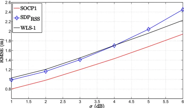
2.1 Simulation results for non-cooperative localization in indoor environment when
P0is known: RMSE (m) versusσ (dB) whenN = 9,U= 5 dB, γ= 2.4,γw= 4
dB, d0= 1 m, P0=−10 dBm, Mc= 50000. . . 25
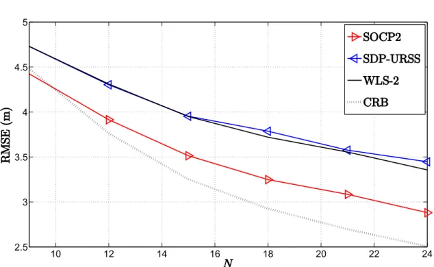
2.2 Simulation results for non-cooperative localization when P0 is not known: RMSE (m) versus N when σ = 5 dB, B = 15 m, r= 20 m, P0=−10 dBm, γ= 3, d0= 1 m, Mc= 10000. . . 27
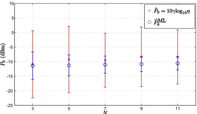
2.3 Simulation results for non-cooperative localization when P0 is not known: ˆP0 (dBm) versus N whenσ= 6 dB,B= 15 m,P0=−10 dBm,γ= 2.5,d0= 1 m, Mc= 1000. . . 28
2.4 Simulation results for non-cooperative localization when P0 and γ are not known: RMSE (m) versus N whenσ= 5 dB, B= 15 m, r= 20 m, P0=−10 dBm,d0= 1 m, Kmax= 30, γmin= 2,γmax= 4,ǫ= 10−3and Mc= 10000. . . 29
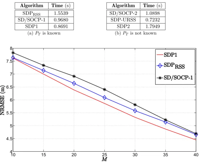
2.5 Simulation results for cooperative localization whenP0 is known: NRMSE (m) versus M whenN = 9, σ= 5 dB,B= 15 m, P0=−10 dBm, γ= 3, d0= 1 m, Mc= 10000. . . 31
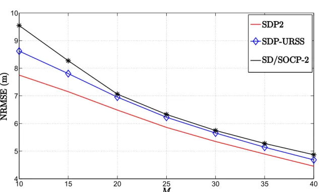
2.6 Example of (a) a network configuration and (b) estimation accuracy results for the “SDP2” approach. Black squares represent the locations of the anchors, blue circles represents the true locations of the targets and red symbols “X” represent the estimated targets. . . 32 2.7 Simulation results for cooperative localization whenP0 is not known: NRMSE
(m) versus M when N = 9, R= 6 m, σ= 5 dB, B = 15 m, P0=−10 dBm, γ= 3, d0= 1 m, Mc= 10000. . . 33
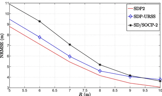
2.9 Simulation results for cooperative localization whenP0 is not known: NRMSE (m) versus N whenM = 15, R= 6 m, σ= 5 dB, B= 15 m, P0=−10 dBm, γ = 3, d0= 1 m, Mc= 10000. Anchors and targets are randomly deployed
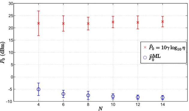
inside the square region of length 2B. . . 35 2.10 Simulation results for non-cooperative localization when P0 is not known: ˆP0
(dBm) versus N whenσ= 6 dB,B= 15 m,P0=−10 dBm,γ= 2.5,d0= 1 m, Mc= 1000. . . 36
2.11 Simulation results for cooperative localization when P0 is not known: CDF of ME (m) in target location estimation when N = 9,M = 15,R= 10 m, σ= 5 dB, B= 15 m,P0=−10 dBm,γ= 3, d0= 1 m, Mc= 10000. . . 37
2.12 A possible second-order coloring scheme for a network with |V|= 13 sensors. 41 2.13 Illustration of the cost functions (2.28) and (2.31) versusx andy coordinates
(target location); the minimum of the cost function is indicated by a white square. . . 44 2.14 Simulation results for cooperative localization when P0 is known: NRMSE (m)
versus kcomparison for differentN, whenM= 50,σ= 0 dB,R= 6 m, B= 30 m, P0=−10 dBm,γ= 3, d0= 1 m, Mc= 500. . . 50
2.15 Simulation results for cooperative localization when P0 is known: NRMSE (m) versus kcomparison for differentM, whenN = 25,σ= 0 dB,R= 6 m, B= 30 m, P0=−10 dBm,γ= 3, d0= 1 m, Mc= 500. . . 51
2.16 Simulation results for cooperative localization when P0 is known: NRMSE (m) versus k comparison for different σ (dB), when N = 25, M = 50, R= 6 m,
B= 30 m, P0=−10 dBm,γ= 3, d0= 1 m,Kmax= 100, Mc= 500. . . 52
2.17 Simulation results for cooperative localization when P0 is known: NRMSE and ¯
k versusσ comparison, whenN= 25,M = 50,R= 6 m,B= 30 m,P0=−10 dBm,γ= 3, d0= 1 m, Kmax= 100, ǫ= 10−3,Mc= 500. . . 53
2.18 NRMSE (m) versus number of iterations comparison of the proposed approach for different choices ofw. . . 54 2.19 Estimation process of the proposed approach in the first 10 iterations. . . 55 2.20 Simulation results for cooperative localization for known and unknown P0:
NRMSE versus k comparison, when N = 25, M = 50, σ = 0 dB, R = 6 m,
B= 30 m, P0=−10 dBm,γ= 3, d0= 1 m,Mc= 500. . . 56
3.1 Illustration of different localization systems in a 2-D space. . . 61 3.2 Illustration of a target and anchor locations in a 3-D space. . . 63 3.3 Illustration of azimuth angle measurements: short-range versus long-range. . 66 3.4 RMSE (m) versus N comparison, whenσnij= 6 dB, σmij= 10 deg, σvij= 10
deg, γij∈[2.2,2.8], γ= 2.5,B= 15 m, P0=−10 dBm, d0= 1 m, Mc= 50000. 75
3.5 RMSE (m) versusσnij (dB) comparison, whenN = 4,σmij= 10 deg, σvij= 10
3.6 RMSE (m) versusσmij (deg) comparison, whenN= 4, σnij = 6 dB,σvij= 10
deg, γij∈[2.2,2.8], γ= 2.5,B= 15 m, P0=−10 dBm, d0= 1 m, Mc= 50000. 76
3.7 RMSE (m) versusσvij (deg) comparison, when N= 4, σnij= 6 dB, σmij= 10
deg, γij∈[2.2,2.8], γ= 2.5,B= 15 m, P0=−10 dBm, d0= 1 m, Mc= 50000. 77
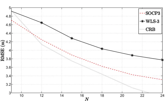
3.8 NRMSE (m) versus N comparison, when M = 20, R = 8 m, σnij = 6 dB,
σmij= 10 deg,σvij= 10 deg,γij∈[2.2,2.8],γ= 2.5,B= 15 m,P0=−10 dBm,
d0= 1 m,Mc= 1000. . . 78
3.9 NRMSE (m) versus M comparison, when N = 8, R = 8 m, σnij = 6 dB,
σmij= 10 deg,σvij= 10 deg,γij∈[2.2,2.8],γ= 2.5,B= 15 m,P0=−10 dBm,
d0= 1 m,Mc= 1000. . . 79
3.10 NRMSE (m) versus R (m) comparison, when N = 8, M = 20, σnij = 6 dB,
σmij= 10 deg,σvij= 10 deg,γij∈[2.2,2.8],γ= 2.5,B= 15 m,P0=−10 dBm,
d0= 1 m,Mc= 1000 . . . 80
3.11 Experimental set-up with 7 anchors (black squares) and 27 targets (blue circles) 80 3.12 Illustration of the RSS peaks, indicating a possible direction of the target. . . 81 3.13 CDF of the LE (m). . . 82 3.14 RMSE (m) versus N performance comparison in the considered experimental
setup. . . 83 3.15 Illustration of a target and anchor locations in a 3-D space. . . 86 3.16 Illustration of the objective functions in (3.31), (3.35) and (3.39) versus x (m)
andy(m) coordinates (target location); the minimum of the objective function is indicated by a white square. . . 92 3.17 NRMSE (m) versus tcomparison, when N= 20, M= 50, R= 6.5 m,σnij = 3
dB, σmij = 6 deg, σvij = 6 deg, γij ∈ U[2.7,3.3], γ = 3, B = 20 m, P0i ∈
U[−12,−8] dBm,d0= 1 m,Mc= 500. . . 98
3.18 NRMSE (m) versus tcomparison, when N= 30, M= 50, R= 6.5 m,σnij = 3
dB, σmij = 6 deg, σvij = 6 deg, γij ∈ U[2.7,3.3], γ = 3, B = 20 m, P0i ∈
U[−12,−8] dBm,d0= 1 m,Mc= 500. . . 98
3.19 NRMSE (m) versus tcomparison, when N= 20, M= 60, R= 6.5 m,σnij = 3
dB, σmij = 6 deg, σvij = 6 deg, γij ∈ U[2.7,3.3], γ = 3, B = 20 m, P0i ∈
U[−12,−8] dBm,d0= 1 m,Mc= 500. . . 99
3.20 NRMSE (m) versus σnij (dB) comparison, when N = 20, M = 50, R= 6.5
m, σmij = 1 deg, σvij = 1 deg, γij ∈U[2.7,3.3], γ = 3, Tmax= 30, B = 20 m,
P0i∈U[−12,−8] dBm, d0= 1 m, Mc= 500. . . 100
3.21 NRMSE (m) versus σmij (deg) comparison, when N = 20, M = 50, R= 6.5
m, σnij = 1 dB, σvij = 1 deg, γij ∈U[2.7,3.3], γ = 3, Tmax= 30, B = 20 m,
P0i∈U[−12,−8] dBm, d0= 1 m, Mc= 500. . . 101
3.22 NRMSE (m) versus σvij (deg) comparison, when N = 20, M = 50, R= 6.5
m, σnij = 1 dB, σmij = 1 deg, γij ∈U[2.7,3.3], γ = 3, Tmax= 30, B = 20 m,
4.1 True target trajectory and mobile sensors’ initial locations. . . 112 4.2 RMSE (m) versus t (s) comparison in the first scenario, whenN = 3, va= 0
m/s, σni = 9 dB, σmi = 4
π
180 rad, γ = 3, γi ∼ U[2.7,3.3], P0 =−10 dBm, q= 2.5×10⁻³m2/s3,Mc= 1000. . . 113
4.3 RMSE (m) versust(s) comparison in the second scenario, when N= 3, va= 0
m/s, σni = 9 dB, σmi = 4
π
180 rad, γ = 3, γi ∼ U[2.7,3.3], P0 =−10 dBm, q= 2.5×10⁻³m2/s3,Mc= 1000. . . 114
4.4 Illustration of the estimation process in the first scenario, whenN = 2,va= 1
m/s, σni = 9 dB, σmi = 4
π
180 rad, γ = 3, γi∼U[2.7,3.3], τ = 5 m, P0=−10 dBm,q= 2.5×10⁻³m2/s3. . . 114 4.5 RMSE (m) versus t (s) comparison in the first scenario, whenN = 2, va= 1
m/s, σni = 9 dB, σmi = 4
π
180 rad, γ = 3, γi∼U[2.7,3.3], τ = 5 m, P0=−10 dBm,q= 2.5×10⁻³m2/s3,Mc= 1000. . . 115
4.6 Pb¯0 (dBm) versus t (s) comparison in the first scenario, when N = 2, va = 0
m/s, σni = 9 dB, σmi = 4
π
180 rad, γ = 3, γi∼U[2.7,3.3], τ = 5 m, P0=−10 dBm,q= 2.5×10⁻³m2/s3,Mc= 1000. . . 116
4.7 Illustration of the estimation process in the second scenario, whenN= 2,va= 1
m/s, σni = 9 dB, σmi = 4
π
180 rad, γ = 3, γi∼U[2.7,3.3], τ = 5 m, P0=−10 dBm,q= 2.5×10⁻³m2/s3. . . 116 4.8 RMSE (m) versust(s) comparison in the second scenario, when N= 2, va= 1
m/s, σni = 9 dB, σmi = 4
π
180 rad, γ = 3, γi∼U[2.7,3.3], τ = 5 m, P0=−10 dBm,q= 2.5×10⁻³m2/s3,Mc= 1000. . . 117
4.9 Pb¯0 (dBm) versust (s) comparison in the second scenario, whenN = 2,va= 0
m/s, σni = 9 dB, σmi = 4
π
180 rad, γ = 3, γi∼U[2.7,3.3], τ = 5 m, P0=−10 dBm,q= 2.5×10⁻³m2/s3,Mc= 1000. . . 117
4.10 RMSE (m) versus va (m/s) comparison in the first scenario, when N = 2, σni = 9 dB, σmi = 4
π
180 rad, γ = 3, γi∼U[2.7,3.3], τ = 5 m, P0=−10 dBm, q= 2.5×10⁻³m2/s3,Mc= 1000. . . 118
4.11 RMSE (m) versus va (m/s) comparison in the second scenario, when N = 2, σni = 9 dB, σmi = 4
π
180 rad, γ = 3, γi∼U[2.7,3.3], τ = 5 m, P0=−10 dBm, q= 2.5×10⁻³m2/s3,Mc= 1000. . . 119
2.1 Summary of the Considered Algorithms in Section 2.2.2 for knownPT . . . . 25
2.2 Summary of the Considered Algorithms in Section 2.2.2 for unknownPT . . . 26
2.3 P0Estimation Analysis for “SOCP2” Approach . . . 26
2.4 Summary of the Considered Algorithms in Subsection 2.2.2 for unknown PT and γ . . . 28
2.5 Unknown Parameter Estimation Analysis for a Random Choice of ˆγ0∈[γmin, γmax] 29 2.6 Summary of the Considered Algorithms in Section 2.2.3 for knownPT . . . . 30
2.7 The Average Running Time of the Considered Algorithms for the Cooperative Localization. N = 8, M = 20, R= 6 m. CPU: Intel(R)Core(TM)i7-363QM 2.40 GHz. . . 31
2.8 Summary of the Considered Algorithms in Section 2.2.3 for unknownPT . . . 31
2.9 Summary of the Considered Algorithms . . . 49
2.10 The Average Running Time Per Sensor Per Mc Run of the Considered Algo-rithms for known PT, when N = 25, M= 50, σ = 0 dB,R= 6 m, Mc= 100. CPU: Intel(R)Core(TM)i7-363QM 2.40 GHz. . . 51
2.11 The Average Energy Depletion of the Considered Algorithms for Known PT, when N= 25, M= 50, σ= 0 dB,R= 6 m,Mc= 100. . . 52
3.1 Summary of the Considered Algorithms . . . 73
3.2 Computational Complexity of the Considered Algorithms . . . 95
AoA angle of arrival.
BS base station.
CDF cumulative distribution function.
CRB Cramer-Rao lower bound.
FIM Fisher information matrix.
GNSS global navigation satellite system.
GPS global positioning system.
GTRS generalized trust region sub-problem.
KF Kalman filter.
LAN local area network.
LE localization error.
LoS line-of-sight.
LS least squares.
MAC medium access control.
MDS multidimensional scaling.
ME mean error.
MEMS micro-electro-mechanical systems.
ML maximum likelihood.
NLoS non-line-of-sight.
NRMSE normalized root mean square error.
PDF probability density function.
PF particle filter.
PLE Path loss exponent.
RF radio frequency.
RMSE root mean square error.
RSS received signal strength.
RSSD received signal strength difference.
RTT round-trip time.
SDC semidefinite cone.
SDP semidefinite programming.
SoA state of the art.
SOCC second-order cone constraint.
SOCP second-order cone programming.
SR squared range.
STD standard deviation.
TDoA time-difference of arrival.
ToA time of arrival.
ToF time of flight.
UT unscented transformation.
WLAN wireless local area network.
WLS weighted least squares.
For reference purposes, some of the most common symbols used throughout the thesis are listed below. Throughout the thesis, upper-case bold type, lower-case bold type and regular type are used for matrices, vectors and scalars, respectively.
R the set of real numbers
Rn n-dimensional real vectors
Rm×n m×nreal matrices [A]ij the ij-th element ofA AT the transpose of A A−1 the inverse ofA
tr(A) the trace of A
AB the matrix A−B is positive semidefinite
A⊗B the Kronecker product ofA and A In the n×nidentity matrix
0m×n the m×nmatrix of all zero entries
1n the n-dimensional column vector with all entries equal to one
ei the i-column of an identity matrix
diag(x) the square diagonal matrix with the elements of vector xas its main diagonal, and zero elements outside the main diagonal
kxk the Euclidean norm of vector x;kxk=√xTx, wherex∈Rn is a column vector
p(·) probability density function
∼ distributed according to ≈ approximately equal to
C
h
a
p
t
1
I nt r o d u c t i o n
1.1
Motivation
Wireless sensor network (WSN) generally refers to a wireless communication network which is composed of a number of devices, called sensors, allocated over a monitored region in order to measure some local quantity of interest [1]. Due to their autonomy in terms of human interaction and low device costs, WSNs find application in various areas, like event detection (fires, floods, hailstorms) [2], monitoring (industrial, agricultural, health care, environmental) [3, 4], energy-efficient routing [5], exploration (deep water, underground, outer space) [6], and surveillance [7] to name a few. Recent advances in radio frequency (RF) and micro-electro-mechanical systems (MEMS) permit the use of large-scale networks
with hundreds or thousands of nodes [1].
In many practical applications (such as search and rescue, target tracking and detection, cooperative sensing and many more), data acquired inside a WSN are only relevant if the referred location is known. Moreover, accurate localization of people and objects in both indoor and outdoor environments enables new applications in emergency and commercial services (e.g. location-aware vehicles [8], asset management in warehouses [9], navigation [10–13], etc.) that can improve safety and efficiency in everyday life, since each individual device in the network can respond faster andbetter to the changes in the environment [14]. Therefore, accurate information about sensors’ locations is a valuable resource, which offers additional knowledge to the user.
each sensor is a possible solution, but it would severely augment the network costs and restrict its applicability [16]. Besides, GPS is ineffective in indoor, dense urban and forest environments or canyons [17]. In order to maintain low implementation costs, only a small fraction of sensors are equipped with GPS receivers (called anchors), while the remaining ones (called targets) determine their locations by using a kind of localization scheme that takes advantage of the known anchor locations [18]. Since the sensors have minimal processing capabilities, the key requirement is to develop localization algorithms that are fast, scalable and abstemious in their computational and communication requirements. Also, making use of existing technologies (such as terrestrial RF sources) when providing a solution to the object localization problem is strongly encouraged. Nevertheless, WSNs are subject to changes in topology (e.g. node mobility, adding nodes, node and/or link failures), which aggravates the development of even the simplest algorithms.
The idea of wireless positioning was initially conceived for cellular networks, since it invokes many innovative applications and services for its users. Nowadays, rapid increase of heterogeneous smart-devices (mobile phones, tablets) which offer self-sustained applications and seamless interfaces to various wireless networks is pushing the role of the location information to become a crucial component for mobile context-aware applications [18]. Even though we limit our discussion to sensor localization in WSN here, it is worth noting that, in practice, a base station (BS) or an access point in local area network (LAN) can be considered as an anchor, while other devices such as cell phones, laptops, tags,etc., can be considered as targets.
1.2
Localization Schemes
solution for the localization problem [1, 16]. Another attractive low-cost approach might be exploiting RTT measurements, which are easily obtained in wireless local area network (WLAN) systems by using a simple device such as a printed circuit board [26]. Even though RTT systems circumvent the problem of clock synchronization between nodes, the major drawback of this approach is the need for double signal transmission in order to perform a single measurement [27].
Recently, hybrid systems that fuse two measurements of the radio signal have been investigated [26, 28–38]. Hybrid systems profit by exploiting the benefits of combined measurements (more available information), taking advantage of the strongest points of each technique and minimizing their drawbacks. On the other hand, the price to pay for using such systems is the increased complexity of network devices, which increases the network implementation costs [1, 16].
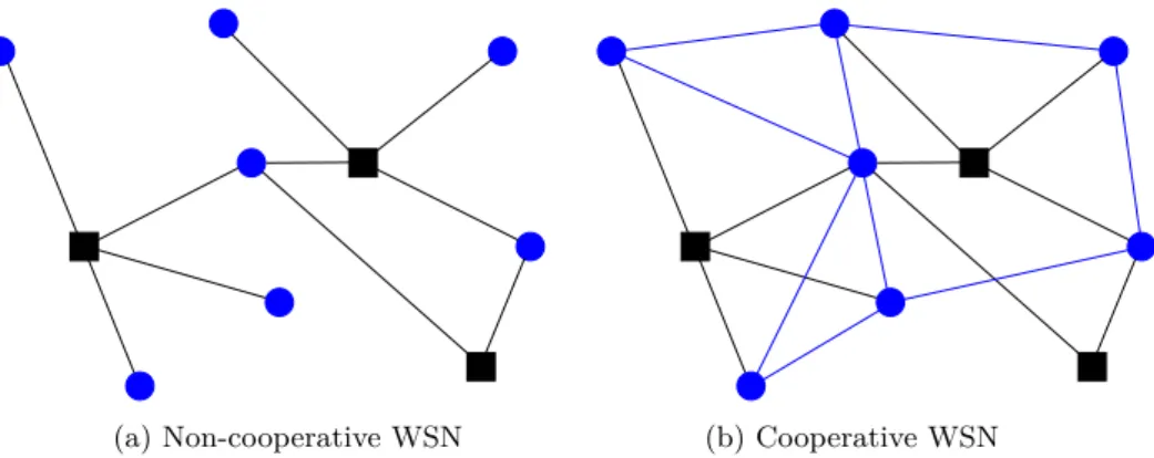
In order to acquire the necessary measurements, node communication is required, which can be non-cooperative or cooperative [18]. The former one allows targets to communicate with the anchors exclusively, Fig. 1.1a, while the latter one allows targets to communicate with all sensors inside their communication range, whether they are anchors or targets, Fig. 1.1b.
(a) Non-cooperative WSN (b) Cooperative WSN
Figure 1.1: Example of a WSN with three anchors (black squares) and seven targets (blue circles).
sensors in some practical applications [39]. On the other hand, the latter approach is distin-guished by low computational complexity and high-scalability, which makes it a preferable solution for large-scale and highly-dense networks [18]. However, distributed algorithms are executed iteratively, which makes them sensitive to error propagation and raises energy consumption. When determining which approach to use for a given application, one has to take into consideration all of the above properties, but if often comes down to efficiency comparison in terms of energy consumtpion. In general, when the average number of hops to the central processor is higher than the necessary number of iterations required for convergence, the distributed approach is likely to be more energy-efficient and vice versa [1].
1.2.1 Overview of Localization Techniques
A detailed survey on localization algorithms can be found in [40], and a brief overview of the state of the art (SoA) related with each chapter’s discussion will be provided at the beginning of each chapter. Here, a general overview of the most commonly used localization techniques is presented.
Range-free Localization
The most commonly used range-free localization technique is fingerprinting. Generally, it can be described as a multiple hypothesis testing decision problem, where the objective is to deduce the best hypothesis (location of the target) based on previously acquired observations, i.e., fingerprints. In practice, a fingerprinting localization method requires two phases: the training and the localization phase. During the training phase, fingerprints are collected at all sample locations [41]. During the localization phase, an obtained radio measurement is compared with all observations collected at sample locations, and the best fit sample location is taken as the estimated target location.
On the one hand, the main advantage of this technique is the flexibility to any radio interface. On the other hand, the localization accuracy depends on the reliability (quantity and up-to-date) of the training data, the error in the synthesis of the fingerprint parameters, and the sensitivity of the algorithm to changes of the environment.
To improve the robustness of the location estimation with respect to the inaccuracy of training data, several techniques are proposed in the literature. For instance, in [42] statistical learning is used to design an algorithm based on support vector machine.
Range-based Localization
Global Navigation Satellite System. A very popular way for determining target’s location nowadays is through a global navigation satellite system (GNSS). It can deliver to its user the latitude and longitude position in real-time [1]. GNSS utilizes satellites orbiting the Earth, which broadcast signals using very precise frequencies and highly-accurate atomic clocks for time measurements. Any receiver on the ground can pick up the GNSS signal as long they are codded to read its signal. As the GNSS signals travel through the Earth’s atmosphere, they can become distorted, leading to a reduced positional accuracy delivered to the receiver. Also, GNSS signals that are low on the horizon, i.e., the ones that have low zenith are more likely to deliver error because they are traveling through more atmosphere. GNSS uses groups of satellites, called constellations, for their systems, see Fig. 1.2. For a receiver to establish its location, it must be able to pick up a signal from at least four of the satellites [43]. Currently, there are two globally operational GNSSs: American GPS (constellation of 32 satellites, fully operational since 1995) and Russian GLONASS (constellation of 24 satellites, restored in 2011). Also, The European Union’s Galileo GNSS, as well as China’s BeiDou-2 GNSS are scheduled to be fully operational by 2020. These systems can be used for providing location, navigation or for tracking the location of a receiver. The signals also allow the electronic receiver to calculate the current local time to high precision, which allows time synchronization. Although technologies like telephonic or internet reception could be used to further enhance the localization performance of GNSSs, they usually operate independently of any of them. Also, even though these systems represent today a standard solution for outdoor localization, they have very limited or no functionality in harsh propagation environments, such as dense urban, underground, underwater and indoor to name a few [43].
Figure 1.2: Example of a GNSS constellation.
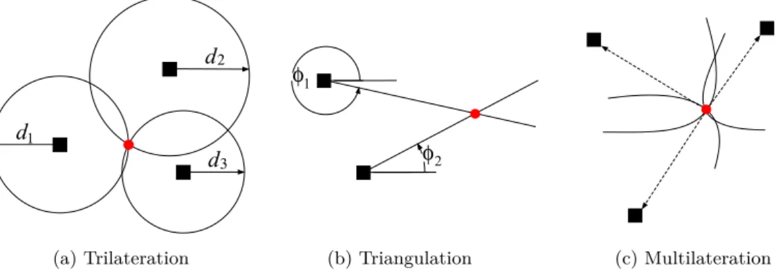
Then, by using at least three anchors in 2-dimensional space, it locates the target by calculating the intersection of the circles based on simultaneous range measurements from anchors, Fig.1.3a. Triangulation is used when the direction of target instead of the distance is estimated, Fig.1.3b. The target location is determined by using the trigonometry laws of sine and cosine [45]. Multilateration is a technique based on the measurement of the difference in distance to two or more anchors which form a hyperbolic curve [46]. The intersection of the hyperbolas, corresponding to the TDoA measurements, determines the position of the target, Fig.1.3c.
d
d
d
1
3 2
(a) Trilateration
φ
φ 1
2
(b) Triangulation (c) Multilateration
Figure 1.3: Illustration of geometric localization techniques.
In practice however, due to noise in radio measurements, the position lines intersect at multiple points instead of a single one. In this case, geometric approach does not provide a useful insight as to which intersection point to choose as the location of the target.
Optimization-based Techniques. If data are known to be well described by a certain statis-tical model, then the maximum likelihood (ML) estimator can be derived and implemented. This is because the variance of these estimators approaches asymptotically (as the signal-to-noise ratio goes high) a lower bound given by the Cramer-Rao lower bound (CRB) [47]. Typically, ML solutions are obtained as the global minimum of the non-convex objective function which is directly derived from the likelihood function of the problem. Even though a closed form ML solution is not possible because of non-linear dependence between the measurements and the unknown parameters, approximate and iterative ML techniques can be derived.
proportional to the grid size and require a huge amount of memory when the number of the unknown parameters is too large. Linear estimators are very efficient in the sense of time-consumption and computational complexity, but they are derived based on many approximations which may severely affect their performance, especially in the case when the noise is large [52]. Convex relaxation techniques overcome the difficulties in the ML problem by transforming the original non-convex and non-linear problem into a convex one. The advantage of this approach is that the convergence to the globally optimal solution is guaranteed. However, due to application of relaxation techniques, the solution of a convex problem does not necessarily correspond to the solution of the original ML problem [57].
1.3
Research Question and General Approach
In this thesis, we investigate both RSS- and combined RSS-AoA-based target localization problems in non-cooperative and cooperative WSNs, and we consider both centralized and distributed types of algorithm execution. Furthermore, we also study the target tracking problem by taking advantage of coupled, RSS and AoA, measurements for both cases of fixed anchors and mobile sensors. In addition, various settings of the localization problem are of interest, such as:
• Only target’s coordinates are not known;
• Target’s coordinates and transmit power are simultaneously not known; • Path loss exponent (PLE) is perfectly and imperfectly known;
• Synchronous node communication managed by a central node or by a kind of medium access control (MAC) protocol;
• Distinct target trajectories in the case of target tracking; • Different velocities of the mobile sensors.
Moreover, in practice, WSNs are subject to changes in topology (e.g., node and/or link failure) and in indoor and highly dense urban environments, mixture of line-of-sight (LoS) and non-line-of-sight (NLoS) links is likely to occur. Also, energy resources are often limited by sensor’s battery, and the quality of the measurements by hardware imperfections and noise.
These advents and restrictions aggravate considerably the development of even the simplest algorithms. Therefore, by taking all of the mentioned challenges into consideration, the main research question of this thesis is:
To address the above research question, the research presented in the thesis commenced from the following hypothesis.
An efficient localization algorithm can be developed by using statistical modelling and convex optimization tools in order to tightly approximate the original non-linear and non-convex localization problem into a convex one. In addition, node cooperation and MAC schemes can be exploited in order to obtain a sufficient amount of information and prevent message collision (re-transmission), respectively. Also, by careful devel-opment of weighting strategy, the influence of potentially bad links can be minimized and the influence of potentially good ones enhanced. Furthermore, by integrating prior knowledge within an estimator and by designing a sensors navigation routine, the performance of an estimator can be improved significantly.
Simulation and experimental results provided within the thesis, as well as a notable number of publications that have arisen from it, verify the probity of the above hypothesis.
1.4
Thesis Outline and Contributions
The thesis is organized into 4 chapters. We summarize the content of each chapter, besides the current one which gives the motivation and outline of this dissertation. Since the thesis is based on ardent and dedicated research which resulted in several publications in international journals and conferences, and book chapters, for each chapter, we also refer the publications (journal papers (J), books (B), book chapters (BC), conference papers (C), and patents (P)) that it has given rise.
In more detail, the outline and the original contributions of this thesis are as follows.
message re-transmission are applied. Finally, a heuristic approach which improves the convergence rate of the new algorithm is discussed.
Publications. The results of this work have been published in:
J1 S. Tomic, M. Beko, and R. Dinis, “Distributed RSS-Based Localization in Wireless Sensor Networks Based on Second-Order Cone Programming,”Sensors, vol. 14, no. 10, pp. 18410–18432, Oct. 2014.
J2 S. Tomic, M. Beko, and R. Dinis, “RSS-based Localization in Wireless Sensor Networks Using Convex Relaxation: Noncooperative and Cooperative Schemes,” IEEE Trans. Veh. Technol.,vol. 64, no. 5, pp. 2037–2050, May 2015.
C1 S. Tomic, M. Beko, R. Dinis, V. Lipovac, “RSS-based Localization in Wireless Sensor Networks using SOCP Relaxation,” In Proc. IEEE 14th Workshop on Signal Processing Advances in Wireless Communications (SPAWC), Darmstadt, Germany, June 16-19, 2013.
C2 S. Tomic, M. Beko, R. Dinis, V. Lipovac, G. Dimic, “RSS-based Localization in Wireless Sensor Networks with Unknown Transmit Power and Path Loss Exponent using SDP Relaxation,” In Proc. WSEAS International Conference on Applied Electromagnetics, Wireless and Optical Communications (ELEC-TROSCIENCE), Dubrovnik, Croatia, June 25-27, 2013.
C3 S. Tomic, M. Beko, R. Dinis, M. Raspopovic, “Distributed RSS-based Local-ization in Wireless Sensor Networks using Convex Relaxation,” In Proc. Inter-national Conference on Computing, Networking and Communications (ICCNC), Hawaii, USA, February 3-6, 2014.
C4 S. Tomic, M. Beko, R. Dinis, M. Raspopovic, “Distributed RSS-based Localiza-tion in Wireless Sensor Networks with Asynchronous Node CommunicaLocaliza-tion,” In Proc. 5th Doctoral Conference on Computing, Electrical and Industrial Systems (DoCEIS), Caparica, Portugal, April 7-9, 2014.
C5 S. Tomic, M. Marikj, M. Beko, R. Dinis, M. Raspopovic, R.Sendelj, “Energy-efficient Distributed RSS-based Localization in Wireless Sensor Networks Using Convex Relaxation,” In Proc. 6th International ICT Forum, Nis, Serbia, Octo-ber 14-16, 2014.
C6 S. Tomic, M. Beko, R. Dinis, G. Dimic, M. Tuba, “Distributed RSS-based Localization in Wireless Sensor Networks with Node Selection Mechanism,” In Proc. 6th Doctoral Conference on Computing, Electrical and Industrial Systems (DoCEIS), Caparica, Portugal, April 13-15, 2015.
Chapter 3. RSS-AoA-based Target Localization: This chapter tackles the target lo-calization problem by measurement fusion. More precisely, hybrid RSS and AoA measurements are integrated in order to enhance the estimation accuracy in com-parison with traditional approach. By using the RSS propagation model and simple geometry, a novel objective function based on the LS criterion is derived. For non-cooperative and non-cooperative WSN, the objective function is then transformed into a generalized trust region sub-problem (GTRS) and an SDP framework, respectively. Moreover, the original non-convex target localization problem is broken down into local sub-problems, which are converted into convex problems by applying SOCP re-laxation technique. By solving this tight approximation of the original problem, each target estimates its own location, resorting only to local information from one-hop neighbors by following our described iterative procedure. Besides excellent trade-off between accuracy and computational cost, the new algorithms have a big advantage over existing approaches as their adaptation to different settings of the localization problem is straightforward.
Publications. The results of this work have been published in:
J3 S. Tomic, M. Beko and R. Dinis, “3-D Target Localization in Wireless Sensor Network Using RSS and AoA Measurement,” IEEE Trans. Vehic. Technol., vol. 66, no. 4, pp. 3197-3210, Apr. 2017.
J4 S. Tomic, M. Beko, and R. Dinis, “Distributed RSS-AoA Based Localization with Unknown Transmit Powers,”IEEE Wirel. Commun. Letters, vol. 5, no. 4, pp. 392–395, Aug. 2016.
J5 S. Tomic, M. Beko, and R. Dinis, “Distributed Algorithm for Target Localization in Wireless Sensor Networks Using RSS and AoA Measurements,” Elsevier Journal on Pervasive and Mobile Computing, vol. 37, pp. 63–77, Jun. 2017. J6 S. Tomic, M. Beko, and R. Dinis, “A Closed-form Solution for RSS/AoA Target
Localization by Spherical Coordinates Conversion,” IEEE Wirel. Commun. Letters, vol. 5, no. 6, pp. 680–683, Dec. 2016.
B1 S. Tomic, M. Beko, R. Dinis, M. Tuba, N. Bacanin. RSS-AoA-based Target Localization and Tracking in Wireless Sensor Networks. Forthcoming, River Publishers Series in Communications, River Publishers, ISBN: 9788793519886, June 2017.
B2 D. Vicente, S. Tomic, M. Beko. Distributed Algorithms for Target Localization in WSNs Using RSS and AoA Measurement. Forthcoming, Lambert Academic Publishing, ISBN: 9783330085107.
P2 M. Beko, S. Tomic, R. Dinis, and P. Montezuma, “Método para Localiza-ção Tridimensional de Nós Alvo numa Rede de Sensores sem Fio Baseado em Medições de Potência Recebida e Angulos de Chegada do Sinal Recebido,” PT, no. 108963, 2015, pending.
P3 M. Beko, S. Tomic, R. Dinis, and P. Montezuma, “Method for RSS/AoA Target 3-D Localization in Wireless Networks,” USA, no. 15287880, 2016, pending. BC1 S. Tomic, M. Beko, and R. Dinis, “Hybrid RSS/AoA-based Localization of
Target Nodes in a 3-D Wireless Sensor Network,” Sensors & Signals, Eds. S. Y. Yurish, A. D. Malayeri: pp. 71–85, ISBN: 978-84-608-2320-9, Book Series, IFSA Publishing, 2015.
BC2 S. Tomic, M. Beko, and R. Dinis, “Target Localization in Cooperative Wire-less Sensor Networks Using Measurement Fusion,” Advances in Sensors: Re-views. Transducers, Signal Conditioning and Wireless Sensors Networks, Ed. S. Y. Yurish: pp. 329–344, ISBN: 978-84-608-7705-9, Book Series, Vol. 3, IFSA Publishing, 2016.
BC3 S. Tomic, M. Beko, and R. Dinis, “Distributed Algorithm for Multiple Tar-get Localization in Wireless Sensor Networks Using Combined Measurements,” Advances in Sensors: Reviews. Sensors and Applications in Measuring and Automation Control Systems, Ed. S. Y. Yurish: pp. 263–275, ISBN: 978-84-617-7596-5, Book Series, Vol. 4, IFSA Publishing, 2017.
C8 S. Tomic, M. Marikj, M. Beko, R. Dinis, “Hybrid RSS-AoA Technique for 3-D Node Localization in Wireless Sensor Networks,” In Proc. International Wire-less Communications and Mobile Computing Conference (IWCMC), Dubrovnik, Croatia, August 24-28, 2015.
C9 S. Tomic, M. Beko, R. Dinis, L. Berbakov, “Cooperative Localization in Wireless Sensor Networks Using Combined Measurements,” In Proc. Telecom-munications Forum (TELFOR), Belgrade, Serbia, November 24-26, 2015. C10 S. Tomic, M. Beko, R. Dinis, M. Tuba, “A WLS Estimator for Target
Localization in a Cooperative Wireless Sensor Network,” In Proc. 7th Doc-toral Conference on Computing, Electrical and Industrial Systems (DoCEIS), Caparica, Portugal, April 11-13, 2016.
C11 S. Tomic, M. Beko, R. Dinis, M. Tuba, N. Bacanin, “An Efficient WLS Esti-mator for Target Localization in Wireless Sensor Networks,” In Proc. Telecom-munications Forum (TELFOR), Belgrade, Serbia, November 22-23, 2016.
between the unknown target location and gathered measurements are established by applying Cartesian to polar coordinates conversion, which results in efficient lin-earization of the highly non-linear observation model. By taking advantage of the linearized observation model and following the MAP criterion and Kalman filter (KF) recipe, novel MAP and KF algorithms are derived which efficiently solve the target tracking problem with static anchors. The target tracking problem is then extended to the case where the target transmit power is not known. Also, the case where sensors’ mobility is granted is studied, and a simple navigation routine is developed, which additionally betters the estimation accuracy, even for lower number of sensors.
Publications. The results of this work have been submitted to:
J7 S. Tomic, M. Beko, and R. Dinis, “Bayesian Methodology for Target Tracking Using RSS and AoA Measurements,” Submitted to Elsevier Journal on Ad Hoc Networks, Dec. 2016.
J8 S. Tomic, M. Beko, and R. Dinis, “Target Tracking With Sensor Navigation Using Coupled RSS and AoA Measurements,” Submitted to Elsevier Journal on Signal Processing,Dec. 2016.
C12 S. Tomic, M. Beko, R.Dinis, M. Tuba, and N.Bacanin, “MAP Estimator for Target Tracking in Wireless Sensor Networks for Unknown Transmit Power,” In Proc. 8th Doctoral Conference on Computing, Electrical and Industrial Systems (DoCEIS), Caparica, Portugal, May 03-05, 2017.
C13 S. Tomic, M. Beko, R.Dinis, M. Tuba, and N.Bacanin, “Kalman Filter for Target Tracking Using Combined RSS and AoA Measurements,” To appear in 13th International Wireless Communications and Mobile Computing Conference (IWCMC), Valencia, Spain, June 26-30, 2017.
C
h
a
p
t
2
R S S - b a s e d Ta r g e t L o c a l i z a t i o n
2.1
Chapter Summary
This chapter addresses the problem of target localization by using RSS measurements. It is organized into two main sections in which we investigate both centralized, Section 2.2, and distributed, Section 2.3, localization problem, respectively. More specifically, the remainder of the chapter is organized as follows.
Section 2.2.1 offers an overview of the related work in the area of RSS-based target localization, as well as our contributions in that area. In Section 2.2.2, the RSS mea-surement model for locating a single target is introduced, centralized target localization problem is formulated for the case of known target transmit power and development of our centralized SOCP estimator is presented. We then extend this approach for the case where PT, and PT and PLE are simultaneously unknown. Section 2.2.3 introduces the
RSS measurement model for the cooperative localization where multiple targets are lo-cated simultaneously. We provide a formulation of the centralized cooperative localization problem and provide details about the development of our SDP estimators for both cases of known and unknown target transmit power. The complexity analysis is summarized in Section 2.2.4. In Section 2.2.5 we provide both complexity and simulation results to compare the performance of our estimators with existing ones. Finally, in Section 2.2.6 we summarize the main conclusions regarding the centralized RSS-based localization problem.
Section 2.3.1 relates the SoA of the distributed RSS-based localization problem, and sums up our contributions in the area. In Section 2.3.2 the local ML optimization prob-lem for locating multiple targets is formulated. Section 2.3.3 provides details about the development of our distributed SOCP estimator for both cases of known and unknown
PT. Computational complexity and energy consumption analysis are summarized in
simulation results to compare the performance of our distributed estimator with existing ones. Finally, in Section 2.3.6 we summarize the main conclusions regarding the distributed RSS-based localization problem.
2.2
Centralized RSS-based Target Localization
2.2.1 Related Work
Target localization based on the RSS measurements has recently attracted much attention in the wireless communications community [48–56]. The most popular estimator used in practice is the ML estimator, since it is asymptotically efficient (for large enough data records) [47]. However, solving the ML estimator of the RSS-based localization problem is a very difficult task, because it is highly non-linear and noncovex [16], hence it may have multiple local optima. In this case, search for the globally optimal solution is very hard via iterative algorithms, since they may converge to a local minimum or a saddle point resulting in a large estimation error. To overcome this difficulty, and possibly provide a good initial point (close to the global minimum) for the iterative algorithms, approaches such as grid search methods, linear estimators, and convex relaxation techniques have been introduced to address the ML problem [48–56]. The grid search methods are time-consuming and require huge amount of memory when the number of the unknown parameters is too large. Linear estimators are very efficient in the sense of time-consumption, but they are derived based on many approximations which may affect their performance, especially in the case when the noise is large [52]. In convex relaxation techniques such as the ones of [50]-[56], the difficulties in the ML problem are overcome by transforming the original non-convex and non-linear problem into a convex one. The advantage of this approach is that the convergence to the globally optimal solution is guaranteed. However, due to the use of relaxation techniques, the solution of a convex problem does not necessarily correspond to the solution of the original ML problem [57].
In [48], different weighting schemes for multidimensional scaling (MDS) formulation were presented and compared. It was shown that the solution of the MDS can be used as the initial value for iterative algorithms, which then converge faster and attain higher accuracy when compared with random initial values. Convex SDP estimators were proposed in [50] to address the non-convexity of the ML estimator, for both non-cooperative and cooperative localization problems with known target transmit power, PT. The authors
in [50] reformulate the localization problem by eliminating the logarithms in the ML formulation and approaching the localization problem as a minimax optimization one, which is then relaxed as an SDP. Even though the approach described in [50] provides good estimation results, especially for the case of cooperative localization, it has high computational complexity, which might restrict its application in large scale WSNs. In [51], the RSS-based localization problem for known PT was formulated as a weighted least
the cooperative localization, the WLS formulation can be relaxed as a mixed SDP/SOCP, whereas for the non-cooperative localization, the WLS problem can be solved by a bisection method. In [54], Wang et al. addressed the non-cooperative RSS localization problem for the case of unknown PT and the PLE. For the case of unknown PT, based on the
UT, a WLS formulation of the problem is derived, which was solved by the bisection method. When both PT and PLE are not known, an alternating estimation procedure
is introduced. However, both [51] and [54] have the assumption of perfect knowledge of the noise standard deviation (STD). This might not be the case in practice, especially in low-cost systems such as RSS where calibration is avoided due to maintaining low system costs [1, 16]. In [56], Vaghefi et al.addressed the RSS cooperative localization problem for unknown PT. The case where the targets have different PT (e.g., due to different antenna
gains) was considered in [56]. The authors solved the localization problem by applying an SDP relaxation technique, and converting the original ML problem into a convex one. Furthermore, in [56] the authors examined the effect of imperfect knowledge of the PLE on the performance of the SDP algorithm, and used an iterative procedure to solve the problem when PT and PLE are simultaneously unknown.
Contributions
In this thesis, the RSS-based target localization problem for both non-cooperative and cooperative scenarios is considered. Instead of solving the ML problem, which is highly non-convex and computationally exhausting to solve globally, we propose a suboptimal approach that provides efficient solution. Hence, we introduce a new non-convex LS estimator which tightly approximates the ML one for small noise. This estimator represents a smoother and simpler localization problem in comparison with the ML one. Applying appropriate convex relaxations to the derived non-convex estimator, novel SOCP and novel mixed SDP/SOCP estimators are proposed for non-cooperative and cooperative localization cases, respectively.
The proposed approach offers an advantage over the existing ones as it allows straightfor-ward adaptation to different scenarios of the RSS localization problem, thereby significantly reducing the estimation error. In both non-cooperative and cooperative scenarios, we first consider the simplest case of the localization problem where PT is known at the anchors.
Next, we consider a more realistic scenario in which we assume that PT is an unknown
parameter and we generalize our approaches for this setting. Finally, we investigate the most challenging scenario of the localization problem whenPT and PLE are simultaneously
unknown at the anchors. In this case, for the non-cooperative localization, we apply an iterative procedure based on the proposed SOCP method in order to estimate all unknown parameters. We also provide details about the computational complexity of the considered algorithms.
not known. In [51, 54] the authors assume that the accurate knowledge of the noise STD is available, which might not be a valid assumption in some practical scenarios. Hence, we consider a more realistic scenario in which the noise STD is not available. In contrast to [56] where an SDP estimator is derived for the case of unknown PT, we derive our
estimators by using SOCP relaxation for the non-cooperative case and mixed SDP/SOCP relaxation for the cooperative case.
2.2.2 Non-cooperative Localization via SOCP relaxation
Let us consider a WSN with N anchors and one target, where the locations of the anchors are respectively denoted by a1, a2, ..., aN and the location of the unknown target is
denoted by x. Without loss of generality, this section focuses on the 2-D scenario, i.e.,
x,a1,a2, ...,aN ∈R2 (the extension for a 3-D scenario is straightforward). For the sake
of simplicity, we assume that all anchors are equipped with omnidirectional antennas and connected to the target. Further, it is assumed that the anchor locations are known. The RSS model between the target and the i-th anchor is defined as [58, 59]
Pi(dBm) =P0−10γlog10k
x−aik d0
+vi,fori= 1, ..., N, (2.1)
where P0 (dBm) represents the power received at a short reference distance d0 (d0 ≤ kx−aik),γ is the PLE, andvi is the log-normal shadowing term modeled as a zero-mean
Gaussian random variable with variance σi2, i.e., vi ∼N 0, σi2
. The model has been validated by a variety of measurement results [59]-[60].
Based on the measurements in (2.1) and Gaussian noise assumption, the ML estimator is found by solving the non-linear and non-convex LS problem when the noise is Gaussian
ˆ
x= arg min x
N
X
i=1 1
σ2
i
Pi−P0+ 10γlog10k
x−aik d0
2
. (2.2)
To solve (2.2), recursive methods, such as Newton’s method, combined with gradient descent method, are often used [47]. However, the objective function may have many local optima, and local search methods may easily get trapped in a local optimum. Hence, in this thesis, we employ convex relaxation to address the non-convexity of the localization problem.
In the remainder of this section, we deal with the case wherePT is known, with the
case wherePT is considered to be an unknown parameter that needs to be estimated, and
a more general problem when PT and PLE are simultaneously unknown.
Non-cooperative scenario with known PT
The target might be designed to measure and report its own calibration data to the anchors, in which case it is reasonable to assume that the target transmission power is known [16]. This corresponds to the case when the reference powerP0, which depends on PT [58], is
For the sake of simplicity, in the rest of the section, we assume that σi2= σ2, for
i= 1, ..., N. When the noise term is sufficiently small, from (2.1) we get
αikx−aik ≈d0, (2.3)
where αi= 10
Pi−P0
10γ . One way for estimating the target location xis via the minimization
of the LS criterion. Thus, according to (2.3), the least squares estimation problem can be formulated as1
ˆ
x= arg min x
N
X
i=1
(αikx−aik −d0)2. (2.4)
Even though problem in (2.4) is non-convex, when αi = d0, for i= 1, ..., N, it can be accurately solved by the SCLP method presented in [61]2. In the further text, we will present a novel approach to solve the problem defined in (2.4).
Defining auxiliary variables z= [z1, ..., zN]T, where zi =αigi−d0 andgi=kx−aik,
from (2.4) we get
minimize x,g,z kzk
2
subject to
gi=kx−aik, zi=αigi−d0, i= 1, ..., N. (2.5) Introducing an epigraph variablet, and relaxing the non-convex constraint gi=kx−aik
as gi≥ kx−aik, yields the following SOCP problem
minimize x,g,z, t t
subject to
k[2z;t−1]k ≤t+ 1, kx−aik ≤gi,
zi=αigi−d0, i= 1, ..., N. (2.6) Problem (2.6) can be efficiently solved by CVX [62], and we will refer to it as “SOCP1” in the further text3.
1A justification for dropping the shadowing term in the propagation model is provided in the following
text. We can rewrite (2.1) as P0−Pi
10γ = log10kx−d0aik+ vi
10γ, which corresponds toαikx−aik=d010
vi
10γ.
For sufficiently small noise, the first-order Taylor series expansion to the right-hand side of the previous expression is given by αikx−aik=d0(1 + ln 1010γvi), i.e., αikx−aik=d0+ǫi, where ǫi=d0ln 1010γvi is the zero-mean Gaussian random variable with the variance d20(ln 10)100γ22σ2. Clearly, the corresponding LS estimator is given by (2.4). Similar has been done in [56].
2It is possible to generalize the SCLP method to the weighted case,i.e., to the case whenα
i,d0 for
some i. However, the algorithm of [61] yields a meaningless solution. This is due to the fact that the almost convexity property of the resulting constraints is not preserved.
3It is worth noting that “SOCP1” approach can be modified to solve the localization problem in a
Non-cooperative scenario with unknown PT
The assumption that the anchors know the actual target transmission power may be too strong in practice since it would require additional hardware in both target and anchors [16]. In this section, a more realistic and challenging scenario where the anchors are not aware of the target transmission power is considered, thus, P0 is assumed to be unknown and has to be estimated. The joint ML estimation of xand P0can be formulated as
ˆ
θ= arg min θ=[x;P0]
N X i=1 1 σ2 "
Pi−lTθ+ 10γlog10k
ATθ−aik d0
#2
, (2.7)
wherel= [02×1; 1] andA= [I2;01×2].
In (2.3), we assumed that PT, i.e., P0 is known. Assuming that P0 is unknown, we can rewrite (2.3) as
ψikx−aik ≈η d0, (2.8)
whereψi= 10
Pi
10γ andη= 10 P0
10γ. By following a procedure similar to the one in Section 2.2.2
for known PT, we obtain the following SOCP problem
minimize x,g,z, η, t t
subject to
k[2z;t−1]k ≤t+ 1, kx−aik ≤gi,
zi=ψigi−η d0, i= 1, ..., N. (2.9) Even though the approach in (2.9) efficiently solves (2.7), we can further improve its performance. To do so, we will exploit the estimate ofP0,Pb0, which we get by solving (2.9), and solve another SOCP problem. This SOCP approach will be described in the further text.
Introducing auxiliary variablesri=kx−aikandγi=r2i, expanding (2.4) and dropping
the term d20 which has no effect on the minimization, yields
minimize x,γ,r
N
X
i=1
b
α2iγi−2d0αbiri
subject to γi=r2i, ri=kx−aik, i= 1, ..., N, (2.10)
where αbi = 10
b
P0−Pi
10γ . One can relax (2.10) to a convex optimization problem as follows.
The non-convex constraint γi =ri2 will be replaced by the second-order cone constraint
(SOCC)r2i ≤γi. Actually, the inequality constraint ri2≤γi will be satisfied as an equality
since γi andri will decrease and increase in the minimization, respectively. Further, define
an auxiliary variabley=kxk2. The constraint y=kxk2 is relaxed to a convex constraint
y ≥ kxk2 which is evidently a SOCC. With the use of all developed constraints, the problem (2.10) is approximated as a convex, SOCP, optimization problem:
minimize x,γ,r, y
N
X
i=1
b
α2iγi−2d0αbiri
subject to
k[2x;y−1]k ≤y+ 1, k[2ri;γi−1]k ≤γi+ 1,
γi=y−2aTi x+kaik2, i= 1, ..., N. (2.11)
In summary, the proposed procedure for solving (2.7) is given below:
Step 1) Solve (2.9) to obtain the initial estimate of x, ˆx′.
Step 2) Use ˆx′ to compute the ML estimate of P0,Pb0′, from (2.7) as:
b
P0′= PN
i=1
Pi+ 10γlog10kˆ x′−aik
d0
N ; (2.12)
Step 3) Use Pb0′ to solve the SOCP in (2.11) and obtain the new target position estimate x, ˆx′′. Compute the ML estimate of P0,Pb0′′, from (2.12), by using ˆx′′.
The main reason for applying this simple procedure is that, we observed in our simu-lations that after solving (2.9) we obtain an excellent ML estimation of P0,Pb0′, which is very close to the true value ofP0. This motivated us to take advantage of this estimated value and solve another SOCP problem (2.11), as ifPT,i.e.,P0is known. In Section 2.2.5 we will see remarkable improvements in the estimation accuracy of both x and P0 by employing the above procedure. We denote this three-step procedure as “SOCP2”.
Non-cooperative scenario with unknown PT andγ
Signal attenuation may be caused by many effects, such as multipath fading, diffraction, reflection, environment and weather conditions characteristics, etc. Thus, it is reasonable to assume that PLE, i.e.,γ is not known at the anchors. In this subsection we investigate the case where PT and γ are simultaneously unknown at the anchors. The joint ML
estimation of x,P0 and γ is written as
ˆ
θ= arg min θ=[x;P0;γ]
N
X
i=1 1
σ2i
"
Pi−hTθ+ 10gTθlog10k
CTθ−aik d0
#2
, (2.13)
where h= [02×1; 1 ; 0], g= [03×1; 1] and C = [I2;02×2]. Problem (2.13) is non-convex and has no closed form solution. To tackle (2.13), we employ a standard alternating procedure explained below (see also [54] and the references therein):