Predicting SMT Solver Performance for Software Verification

C. Dubois, P. Masci, D. M´ery (Eds.): F-IDE 2016 EPTCS 240, 2017, pp. 20–37, doi:10.4204/EPTCS.240.2

c

A. Healy, R. Monahan & J. F. Power This work is licensed under the Creative Commons Attribution License. Andrew Healy Rosemary Monahan James F. Power

Dept. of Computer Science, Maynooth University, Maynooth, Ireland ahealy@cs.nuim.ie rosemary@cs.nuim.ie jpower@cs.nuim.ie

TheWhy3IDE and verification system facilitates the use of a wide range of Satisfiability Modulo Theories (SMT) solvers through a driver-based architecture. We presentWhere4: a portfolio-based approach to dischargeWhy3proof obligations. We use data analysis and machine learning techniques on static metrics derived from program source code. Our approach benefits software engineers by providing a single utility to delegate proof obligations to the solvers most likely to return a useful result. It does this in a time-efficient way using existingWhy3and solver installations — without requiring low-level knowledge about SMT solver operation from the user.

1

Introduction

The formal verification of software generally requires a software engineer to use a system of tightly integrated components. Such systems typically consist of an IDE that can accommodate both the imple-mentation of a program and the specification of its formal properties. These two aspects of the program are then typically translated into the logical constructs of an intermediate language, forming a series of goals which must be proved in order for the program to be fully verified. These goals (or “proof obliga-tions”) must be formatted for the system’s general-purpose back-end solver. Examples of systems which follow this model are Spec# [3] and Dafny [28] which use the Boogie [2] intermediate language and the Z3 [19] SMT solver.

Why3[22] was developed as an attempt to make use of the wide spectrum of interactive and auto-mated theorem proving tools and overcome the limitations of systems which rely on a single SMT solver. It provides a driver-based, extensible architecture to perform the necessary translations into the input for-mats of two dozen provers. With a wide choice of theorem-proving tools now available to the software engineer, the question of choosing the most appropriate tool for the task at hand becomes important. It is this question thatWhere4answers.

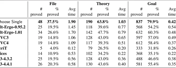
As motivation for our approach, Table 1 presents the results from running the Why3tool over the example programs included in theWhy3distribution (version 0.87.1), using eight SMT solvers at the back-end. EachWhy3file contains a number of theories requiring proof, and these in turn are broken down into a number of goals for the SMT solver; for the data in Table 1 we had 128 example programs, generating 289 theories, in turn generating 1048 goals. In Table 1 each row presents the data for a single SMT solver, and the three main data columns give data totalled on a per-file, per-theory and per-goal basis. Each of these three columns is further broken down to show the number of programs/theories/goals that were successfully solved, their percentage of the total, and the average time taken in seconds for each solver to return such a result. Program verification by modularisation construct is particularly relevant to the use ofWhy3on the command line as opposed to through the IDE.

Table 1: Results of running 8 solvers on the exampleWhy3programs with a timeout value of 10 seconds. In total our dataset contained 128 files, which generated 289 theories, which in turn generated 1048 goals. Also included is a theoretical solverChoose Single, which always returns the best answer in the fastest time.

File Theory Goal

# proved

% proved

Avg time

# proved

% proved

Avg time

# proved

% proved

Avg time

Choose Single 48 37.5% 1.90 190 63.8% 1.03 837 79.9% 0.42

Alt-Ergo-0.95.2 25 19.5% 1.45 118 39.6% 0.77 568 54.2% 0.54

Alt-Ergo-1.01 34 26.6% 1.70 142 47.7% 0.79 632 60.3% 0.48

CVC3 19 14.8% 1.06 128 43.0% 0.65 597 57.0% 0.49

CVC4 19 14.8% 1.09 117 39.3% 0.51 612 58.4% 0.37

veriT 5 4.0% 0.12 79 26.5% 0.20 333 31.8% 0.26

Yices 14 10.9% 0.53 102 34.2% 0.22 368 35.1% 0.22

Z3-4.3.2 25 19.5% 0.56 128 43.0% 0.36 488 46.6% 0.38

Z3-4.4.1 26 20.3% 0.58 130 43.6% 0.40 581 55.4% 0.35

theory or goal. In general, the method of choosing from a range of solvers on an individual goal basis is calledportfolio-solving. This technique has been successfully implemented in the SAT solver domain by SATzilla [38] and for model-checkers [20][36]. Why3presents a unique opportunity to use a common input language to develop a portfolio SMT solver specifically designed for software verification.

The main contributions of this paper are:

1. The design and implementation of our portfolio solver,Where4, which uses supervised machine learning to predict the best solver to use based on metrics collected from goals.

2. The integration ofWhere4into the user’s existingWhy3work-flow by imitating the behaviour of an orthodox SMT solver.

3. A set of metrics to characteriseWhy3goal formulae.

4. Statistics on the performance of eight SMT solvers using a dataset of 1048Why3goals.

Section 2 describes how the data was gathered and discusses issues around the accurate measurement of results and timings. A comparison of prediction models forms the basis of Section 3 where a number of evaluation metrics are introduced. TheWhere4tool is compared to a range of SMT tools and strategies in Section 5. The remaining sections present a review of additional related work and a summary of our conclusions.

2

System Overview and Data Preparation

Alt-Ergo-0.95.2Alt-Ergo-1.01

CVC3 CVC4 _{Yices Z3-4.3.2 Z3-4.4.1 veriT} 0

100 200 300 400 500 600 700 800 900 1000

Number of proof obligations ₅₉₀ 648 613 622

369 502

595 337

144 128 150 ₃₁

415 39

37

331

300 265 230

307 175

174

240 304

14 7 _{55 88 89}

333 176 76

Valid

Unknown

Timeout

Failure

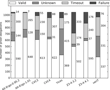
Figure 1: The relative amount ofValid/Unknown/Timeout/Failureanswers from the eight SMT solvers (with a timeout of 60 seconds). Note that no tool returned an answer ofInvalidfor any of the 1048 proof obligations.

are a representative software verification workload. Alternatives to this dataset are discussed in Section 6.

We used six current, general-purpose SMT solvers supported byWhy3: Alt-Ergo [18] versions 0.95.2 and 1.01, CVC3 [6] ver. 2.4.1, CVC4 [4] ver. 1.4, veriT [15], ver. 2015061, Yices [21] ver. 1.0.382, and Z3 [19] ver. 4.3.2 and 4.4.1. We expanded the range of solvers to eight by recording the results for two of the most recent major versions of two popular solvers - Alt-Ergo and Z3.

When a solver is sent a goal by Why3 it returns one of the five possible answers Valid, Invalid, Unknown,TimeoutorFailure. As can be seen from Table 1 and Fig. 1, not all goals can be proved Valid or Invalid. Such goals usually require the use of an interactive theorem prover to discharge goals that require reasoning by induction. Sometimes a splitting transformation needs to be applied to simplify the goals before they are sent to the solver. Our tool does not perform any transformations to goals other than those defined by the solver’sWhy3driver file. In other cases, more time or memory resources need to be allocated in order to return a conclusive result. We address the issue of resource allocation in Section 2.1.1.

2.1 Problem Quantification: predictor and response variables

Two sets of data need to be gathered in supervised machine learning [31]: the independent/predictor vari-ables which are used as input for both training and testing phases, and the dependent/response varivari-ables

Size

ops

divisor conds leaves quants

and

or

not

let

as

eps

func

if

iff

imp

case

var

true

false

wild

zero-ar

int

float

forall

exists

depth

avg-arity

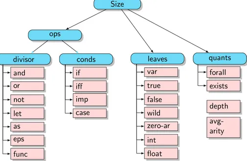
Figure 2: Tree illustrating the Why syntactic features counted individually (pink nodes) while traversing the AST. The rectangles represent individual measures, and the rounded blue nodes represent metrics that are the sum of their children in the tree.

which correspond to ground truths during training. Of the 128 programs in our dataset, 25% were held back for system evaluation (Section 5). The remaining 75% (corresponding to 96 WhyML programs, 768 goals) were used for training and 4-Fold cross-validation.

2.1.1 Independent/Predictor Variables

Fig. 2 lists the predictor variables that were used in our study. All of these are (integer-valued) metrics that can be calculated by analysing a Why3proof obligation, and are similar to the Syntaxmetadata category for proof obligations written in the TPTP format [34]. To construct a feature vector from each task sent to the solvers, we traverse the abstract syntax tree (AST) for each goal and lemma, counting the number of each syntactic feature we find on the way. We focus on goals and lemmas as they produce proof obligations, with axioms and predicates providing a logical context.

Our feature extraction algorithm has similarities in this respect to the method used byWhy3for com-puting goal “shapes” [11]. These shape strings are used internally byWhy3as an identifying fingerprint. Across proof sessions, their use can limit the amount of goals in a file which need to be re-proved.

2.1.2 Dependent/Response Variables

Our evaluation of the performance of a solver depends on two factors: the time taken to calculate that result, and whether or not the solver had actually proven the goal.

measurement introduced at each execution, we used the methodology described by Lilja [30] to obtain an approximation of the true mean time. A 90% confidence interval was used with an allowed error of

±3.5%.

By inspecting our data, we saw that most Valid andInvalid answers returned very quickly, with Unknownanswers taking slightly longer, and Failure/Timeoutresponses taking longest. We took the relative utility of responses to be{Valid,Invalid}>U nknown>{Timeout,Failure}which can be read as “it is better for a solver to return aValidresponse thanTimeout”, etc. A simple function allocates a cost to each solverS’s response to each goalG:

cost(S,G) =   

timeS,G,if answerS,G∈ {Valid,Invalid}

timeS,G+timeout, if answerS,G=U nknown

timeS,G+ (timeout×2), if answerS,G∈ {Timeout,Failure}

Thus, to penalise the solvers that return anUnknownresult, the timeout limit is added to the time taken, while solvers returningTimeoutorFailureare further penalised by adding double the timeout limit to the time taken. A response ofFailurerefers to an error with the backend solver and usually means a required logical theory is not supported. This function ensures the best-performing solvers always have the lowest costs. A ranking of solvers for each goal in order of decreasing relevance is obtained by sorting the solvers by ascending cost.

Since our cost model depends on the time limit value chosen, we need to choose a value that does not favour any one solver. To establish a realistic time limit value, we find each solver’s “Peter Principle Point” [35]. In resource allocation for theorem proving terms, this point can be defined as the time limit at which more resources will not lead to a significant increase in the number of goals the solver can prove.

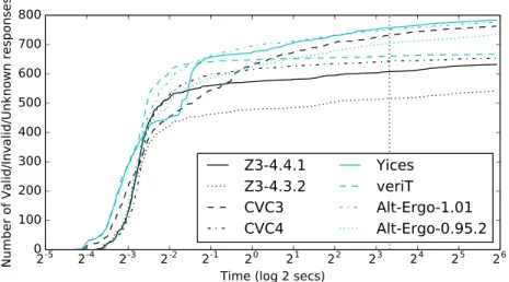
Fig. 3 shows the number ofValid/Invalid/Unknownresults for each prover when given a time limit of 60 seconds. This value was chosen as an upper limit, since a time limit value of 60 seconds is not realistic for most software verification scenarios. Why3, for example, has a default time limit value of 5 seconds. From Fig. 3 we can see that the vast majority of useful responses are returned very quickly.

By satisfying ourselves with being able to record 99% of the useful responses which would be re-turned after 60 seconds, a more reasonable threshold is obtained for each solver. This threshold ranges from 7.35 secs (veriT) to 9.69 secs (Z3-4.3.2). Thus we chose a value of 10 seconds as a representative, realistic time limit that gives each solver a fair opportunity to return decent results.

3

Choosing a prediction model

Given aWhy3goal, a ranking of solvers can be obtained by sorting the cost for each solver. For unseen instances, two approaches to prediction can be used: (1) classification — predicting the final ranking directly — and (2) regression — predicting each solver’s score individually and deriving a ranking from these predictions. With eight solvers, there are 8! possible rankings. Many of these rankings were observed very rarely or did not appear at all in the training data. Such an unbalanced dataset is not appropriate for accurate classification, leading us to pursue the regression approach.

Seven regression models were evaluated3: Linear Regression, Ridge Regression, K-Nearest Neigh-bours, Decision Trees, Random Forests (with and without discretisation) and the regression variant of Support Vector Machines. Table 2 shows the results for some of the best-performing models. Most

2

₂

₂

₂

₂

₂

₂

₂

₂

₂

₂

₂

Time (log 2 secs)

0

100

200

300

400

500

600

700

800

Number of Valid/Invalid/Unknown responses

Z3-4.4.1

Z3-4.3.2

CVC3

CVC4

Yices

veriT

Alt-Ergo-1.01

Alt-Ergo-0.95.2

Figure 3: The cumulative number ofValid/Invalid/Unknownresponses for each solver. The plot uses a logarithmic scale on the time axis for increased clarity at the low end of the scale. The chosen timeout limit of 10 secs (dotted vertical line) includes 99% of each solver’s useful responses

models were evaluated with and without a weighting function applied to the training samples. Weighting is standard practice in supervised machine learning: each sample’s weight was defined as the standard deviation of solver costs. This function was designed to give more importance to instances where there was a large difference in performance among the solvers.

Table 2 also shows three theoretical strategies in order to provide bounds for the prediction models. Bestalways chooses the best ranking of solvers andWorstalways chooses the worst ranking (which is the reverse ordering toBest).Randomis the average result of choosing every permutation of the eight solvers for each instance in the training set. We use this strategy to represent the user selecting SMT solvers at random without any consideration for goal characterisation or solver capabilities. A comparison to a fixedordering of solvers for each goal is not made as any such ordering would be arbitrarily determined. We note that theBesttheoretical strategy of Table 2 is not directly comparable with the theoretical solverChoose Singlefrom Table 1. The two tables’ average time columns are measuring different results: in contrast toChoose Single, Bestwill call each solver in turn, as will all the other models in Table 2, until a resultValid/Invalidis recorded (which it may never be). Thus Table 2’sTimecolumn shows the averagecumulativetime of each such sequence of calls, rather than the average time taken by the single bestsolver called byChoose Single.

3.1 Evaluating the prediction models

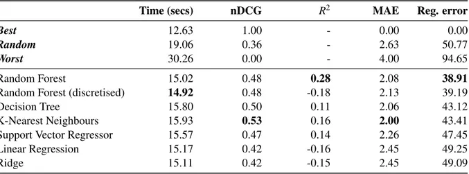
Table 2’sTimecolumn provides an overall estimate of the effectiveness of each prediction model. We can see that the discretised Random Forest method provides the best overall results for the solvers, yielding an average time of 14.92 seconds.

Table 2: Comparing the seven prediction models and three theoretical strategies

Time (secs) nDCG R2 MAE Reg. error

Best _{12.63 1.00 - 0.00 0.00}

Random _{19.06 0.36 - 2.63 50.77}

Worst _{30.26 0.00 - 4.00 94.65}

Random Forest 15.02 0.48 0.28 2.08 38.91

Random Forest (discretised) 14.92 0.48 -0.18 2.13 39.19

Decision Tree 15.80 0.50 0.11 2.06 43.12

K-Nearest Neighbours 15.93 0.53 0.16 2.00 43.41

Support Vector Regressor 15.57 0.47 0.14 2.26 47.45

Linear Regression 15.17 0.42 -0.16 2.45 49.25

Ridge 15.11 0.42 -0.15 2.45 49.09

ranking. For a general ranking of lengthp, it is formulated as:

nDCGp= DCGp

IDCGp where DCGp= p

∑

2reli₋₁

log2(i+1)

Herereli refers to the relevance of element iwith regard to a ground truth ranking, and we take each solver’s relevance to be inversely proportional to its rank index. In our case, p=8 (the number of SMT solvers). TheDCGpis normalised by dividing it by the maximum (oridealised) value for ranks of length p, denotedIDCGp. As our solver rankings are permutations of the ground truth (makingnDCGvalues of 0 impossible), the values in Table 2 are further normalised to the range [0..1] using the lowernDCG bound for ranks of length 8 — found empirically to be 0.4394.

The third numeric column of Table 2 shows the R2 score (or coefficient of determination), which is an established metric for evaluating how well regression models can predict the variance of depen-dent/response variables. The maximumR2 score is 1 but the minimum can be negative. Note that the theoretical strategies return rankings rather than individual solver costs. For this reason,R2 scores are not applicable. Table 2’s fourth numeric column shows theMAE (Mean Average Error) — a ranking metric which can also be used to measure string similarity. It measures the average distance from each predicted rank position to the solver’s index in the ground truth. Finally, the fifth numeric column of Table 2 shows the mean regression error (Reg. error) which measures the mean absolute difference in predicted solver costs to actual values.

3.2 Discussion: choosing a prediction model

An interesting feature of all the best-performing models in Table 2 is their ability to predictmulti-output variables [13]. In contrast to the Support Vector model, for example, which must predict the cost for each solver individually, a multi-output model predicts each solver’s cost simultaneously. Not only is this method more efficient (by reducing the number of estimators required), but it has the ability to account for the correlation of the response variables. This is a useful property in the software verification domain where certain goals are not provable and others are trivial for SMT solvers. Multiple versions of the same solver can also be expected to have highly correlated costs.

metrics (shown in bold) and have generally good scores in the others. Random forests are an ensemble extension of decision trees: random subsets of the training data are used to train each tree. For regression tasks, the set of predictions for each tree is averaged to obtain the forest’s prediction. This method is designed to prevent over-fitting.

Based on the data in Table 2 we selected random forests as the choice of predictor to use inWhere4.

4

Implementing

Where4

in OCaml

Where4’s interaction with Why3is inspired by the use of machine learning in the Sledgehammer tool [10] which allows the use of SMT solvers in the interactive theorem prover Isabelle/HOL. We aspired to Sledgehammer’s ‘zero click, zero maintenance, zero overhead’ philosophy in this regard: it should not interfere with aWhy3user’s normal work-flow nor should it penalise those who do not use it.

We implement a “pre-solving” heuristic commonly used by portfolio solvers [1][38]: a single solver is called with a short time limit before feature extraction and solver rank prediction takes place. By using a good “pre-solver” at this initial stage, easily-proved instances are filtered with a minimum time overhead. We used a ranking of solvers based on the number of goals each could prove, using the data from Table 1. The highest-ranking solver installed locally is chosen as a pre-solver. For the purposes of this paper which assumes all 8 solvers are installed, the pre-solver corresponds to Alt-Ergo version 1.01. The effect pre-solving has on the methodWhere4uses to return responses is illustrated in Alg. 1.

The random forest is fitted on the entire training set and encoded as a JSON file for legibility and modularity. This approach allows new trees and forests devised by the user (possibly using new SMT solvers or data) to replace our model. When the user installsWhere4locally, this JSON file is read and printed as an OCaml array. For efficiency, other important configuration information is compiled into OCaml data structures at this stage: e.g. the user’swhy3.conf file is read to determine the supported SMT solvers. All files are compiled and a native binary is produced. This only needs to be done once (unless the locally installed provers have changed).

TheWhere4command-line tool has the following functionality:

1. Read in the WhyML/Why file and extract feature vectors from its goals.

2. Find the predicted costs for each of the 8 provers by traversing the random forest, using each goal’s feature vector.

3. Sort the costs to produce a ranking of the SMT solvers.

4. Return a predicted ranking for each goal in the file, without calling any solver .

5. Alternatively, use theWhy3API to call each solver (if it is installed) in rank order until aValid/Invalid answer is returned (using Alg. 1).

If the user has selected that Where4 be available for use through Why3, the file which lets Why3 know about supported provers installed locally is modified to contain a new entry for theWhere4binary. A simple driver file (which just tellsWhy3to use the Why logical language for encoding) is added to the drivers’ directory. At this point,Where4can be detected byWhy3, and then used at the command line, through the IDE or by the OCaml API just like any other supported solver.

5

Evaluating

Where4

’s performance on test data

Input:P, aWhy3program;

R, a static ranking of solvers for pre-proving;

φ, a timeout value

Output:hA,Tiwhere

A= the best answer from the solvers; T = the cumulative time taken to returnA

begin

/* Highest ranking solver installed locally */

S←BestInstalled(R)

/* Call solver S on Why3 program P with a timeout of 1 second */ hA,Ti ←Call(P,S,1)

ifA∈ {Valid,Invalid}then returnhA,Ti

end

/* extract feature vector F from program P */

F←ExtractFeatures(P)

/* R is now based on program features */

R←PredictRanking(F)

whileA∈ {/ Valid,Invalid} ∧R6=/0do

S←BestInstalled(R)

/* Call solver S on Why3 program P with a timeout of φ seconds */ hAS,TSi ←Call(P,S,φ)

/* add time TS to the cumulative runtime */ T←T+TS

ifAS>Athen

/* answer AS is better than the current best answer */ A←AS

end

/* remove S from the set of solvers R */

R←R\ {S} end

returnhA,Ti end

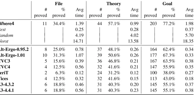
Table 3: Number of files, theories and goals proved by each strategy and individual solver. The percent-age this represents of the total 32 files, 77 theories and 263 goals and the averpercent-age time (in seconds) are also shown.

File Theory Goal

# proved

% proved

Avg time

# proved

% proved

Avg time

# proved

% proved

Avg time

Where4 11 34.4% 1.39 44 57.1% 0.99 203 77.2% 1.98

Best 0.25 0.28 0.37

Random 4.19 4.02 5.70

Worst 14.71 13.58 18.35

Alt-Ergo-0.95.2 8 25.0% 0.78 37 48.1% 0.26 164 62.4% 0.34

Alt-Ergo-1.01 10 31.3% 1.07 39 50.6% 0.26 177 67.3% 0.33

CVC3 5 15.6% 0.39 36 46.8% 0.21 167 63.5% 0.38

CVC4 4 12.5% 0.56 32 41.6% 0.21 147 55.9% 0.35

veriT 2 6.3% 0.12 24 31.2% 0.12 100 38.0% 0.27

Yices 4 12.5% 0.32 32 41.6% 0.15 113 43.0% 0.18

Z3-4.3.2 6 18.8% 0.46 31 40.3% 0.20 145 55.1% 0.37

Z3-4.4.1 6 18.8% 0.56 31 40.3% 0.23 145 55.1% 0.38

5.1 EC1: How doesWhere4perform in comparison to the 8 SMT solvers under consid-eration?

When each solver inWhere4’s ranking sequence is run on each goal, the maximum amount of files, the-ories and goals are provable. As Table 3 shows, the difference betweenWhere4and our set of reference theoretical strategies (Best, Random, andWorst) is the amount of time taken to return theValid/Invalid result. Compared to the 8 SMT provers, the biggest increase is on individual goals: Where4can prove 203 goals, which is 26 (9.9%) more goals than the next best single SMT solver, Alt-Ergo-1.01.

Unfortunately, the average time taken to solve each of these goals is high when compared to the 8 SMT provers. This tells us thatWhere4can perform badly with goals which are not provable by many SMT solvers: expensiveTimeoutresults are chosen before theValidresult is eventually returned. In the worst case,Where4may try and time-out for all 8 solvers in sequence, whereas each individual solver does this just once. Thus, while having access to more solvers allows more goals to be proved, there is also a time penalty to portfolio-based solvers in these circumstances.

At the other extreme, we could limit the portfolio solver to just using the best predicted individual solver (after “pre-solving”), eliminating the multiple time-out overhead. Fig. 4 shows that the effect of this is to reduce the number of goals provable by Where4, though this is still more than the best-performing individual SMT solver, Alt-Ergo-1.01.

To calibrate this cost of Where4 against the individual SMT solvers, we introduce the notion of a cost threshold: using this strategy, after pre-solving, solvers with a predicted cost above this threshold are not called. If no solver’s cost is predicted below the threshold, the pre-solver’s result is returned.

Alt-Ergo-0.95.2

Alt-Ergo-1.01

CVC3 CVC4 veriT Yices Z3-4.3.2Z3-4.4.1

Best RandomWorst Where4

0

50

100

150

200

250

Number of proof obligations

164 177 167 147

_{100 113}

145 145

203

162

62

184

41 36 27

13

38

62 3

4

36

19

13

35

58 50 61

₁₀₃

112

72 107 105

17

89

172

44

0

0

Valid

₈

0

_{13 16 8}

Unknown

₉

Timeout

₇

0

_{16 0}

Failure

Figure 4: The relative amount of Valid/Unknown/Timeout/Failure answers from the eight SMT solvers. Shown on the right are results obtainable by using the top solver (only) with the 3 ranking strategies and theWhere4predicted ranking (with an Alt-Ergo-1.01 pre-solver).

versions of Z3).

5.2 EC2: How does Where4perform in comparison to the 3 theoretical ranking strate-gies?

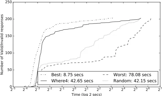
Fig. 6 compares the cumulative time taken forWhere4 and the 3 ranking strategies to return the 203 valid answers in the test set. Although bothWhere4andRandomfinish at approximately the same time, Where4is significantly faster for returningValid/Invalidanswers. Where4’s solid line is more closely correlated toBest’s rate of success than the erratic rate of theRandomstrategy.Best’s time result shows the capability of a perfect-scoring learning strategy. It is motivation to further improveWhere4in the future.

5.3 EC3: What is the time overhead of usingWhere4to proveWhy3goals?

The timings for Where4in all plots and tables are based solely on the performance of the constituent solvers (the measurement of which is discussed in Sec. 2.1.2). They do not measure the time it takes for the OCaml binary to extract the static metrics, traverse the decision trees and predict the ranking. We have found that this adds (on average) 0.46 seconds to the timeWhere4takes to return a result for each file. On a per goal basis, this is equivalent to an increase in 0.056 seconds.

Cost threshold for Where4

0

2

4

6

8

10

12

14

16

18

Time for any response (secs)

0 2 4 6 8 10 12 14 16 18 20

Cost threshold for Where4

100

120

140

160

180

200

220

Number of Valid/ Invalid responses

Where4

Z3-4.4.1

Z3-4.3.2

CVC3

CVC4

Yices

veriT

Alt-Ergo-1.01

Alt-Ergo-0.95.2

2

₂

₂

₂

₂

₂

₂

₂

₂

₂

₂

₂

₂

Time (log 2 secs)

0

50

100

150

200

250

Number of Valid/Invalid responses

_{Best: 8.75 secs}

Where4: 42.65 secs

Worst: 78.08 secs

Random: 42.15 secs

Figure 6: The cumulative time each theoretical strategy, andWhere4to return allValid/Invalidanswers in the test dataset of 263 goals

5.4 Threats to Validity

We categorise threats as either internalorexternal. Internal threats refer to influences that can affect the response variable without the researcher’s knowledge and threaten the conclusions reached about the cause of the experimental results [37]. Threats to external validity are conditions that limit the generalisability and reproducibility of an experiment.

5.4.1 Internal

The main threat to our work’s internal validity is selection bias. All of our training and test samples are taken from the same source. We took care to split the data for training and testing purposes on aper file basis. This ensured thatWhere4was not trained on a goal belonging to the same theory or file as any goal used for testing. The results of running the solvers on our dataset are imbalanced. There were far moreValidresponses than any other response. No goal in our dataset returned an answer ofInvalidon any of the 8 solvers. This is a serious problem asWhere4would not be able to recognize such a goal in real-world use. In future work we hope to use the TPTP benchmark library to remedy these issues. The benchmarks in this library come from a diverse range of contributors working in numerous problem domains [35] and are not as specific to software verification as theWhy3suite of examples.

Use of an independent dataset is likely to influence the performance of the solvers. Alt-Ergo was designed for use with theWhy3platform — its input language is a previous version of the Why logic language. It is natural that the developers of the Why3 examples would write programs which Alt-Ergo in particular would be able to prove. Due to the syntactic similarities in input format and logical similarities such as support for type polymorphism, it is likely that Alt-Ergo would perform well with anyWhy3dataset. We would hope, however, that the gulf between it and other solvers would narrow.

Why logic language (in contrast to related work on model checkers which use the general-purpose C language [20][36]). We made the decision to keep the choice of independent variables simple in order to increase generalisability to other formalisms such as Microsoft’s Boogie [2] intermediate language.

5.4.2 External

The generalisability of our results is limited by the fact that all dependent variables were measured on a single machine.4 We believe that the number of each response for each solver would not vary dramatically on a different machine of similar specifications. By inspecting the results when each solver was given a timeout of 60 seconds (Fig. 3), the rate of increase forValid/Invalidresults was much lower than that ofUnknown/Failureresults. The former set of results are more important when computing the cost value for each solver-goal pair.

Timings of individual goals are likely to vary widely (even across independent executions on the same machine). It is our assumption that although the actual timed values would be quite different on any other machine, therankingof their timings would stay relatively stable.

A “typical” software development scenario might involve a user verifying a single file with a small number of resultant goals: certainly much smaller than the size of our test set (263 goals). In such a setting, the productivity gains associated with usingWhere4 would be minor. Where4 is more suited therefore to large-scale software verification.

5.5 Discussion

By considering the answers to our three Evaluation Criteria, we can make assertions about the success ofWhere4. The answer to EC1, Where4’s performance in comparison to individual SMT solvers, is positive. A small improvement inValid/Invalidresponses results from using only the top-ranked solver, while a much bigger increase can be seen by making the full ranking of solvers available for use. The time penalty associated with calling a number of solvers on an un-provable proof obligation is mitigated by the use of acost threshold. Judicious use of this threshold value can balance the time-taken-versus-goals-proved trade-off: in our test set of 263 POs, using a threshold value of 7 results in 192 Valid responses – an increase of 15 over the single best solver – in a reasonable average time per PO (both Validand otherwise) of 4.59 seconds.

There is also cause for optimism in Where4’s performance as compared to the three theoretical ranking strategies — the subject of Evaluation Criterion 2. All but the most stubborn ofValidanswers are returned in a time far better than Random theoretical strategy. We take this random strategy as representing the behaviour of the non-expertWhy3user who does not have a preference amongst the variety of supported SMT solvers. For this user,Where4could be a valuable tool in the efficient initial verification of proof obligations through theWhy3system.

In terms of time overhead — the concern of EC3 — our results are less favourable, particularly when Where4is used as an integrated part of theWhy3toolchain. The costly printing and parsing of goals slows Where4 beyond the time overhead associated with feature extraction and prediction. At present, due to the diversity of languages and input formats used by software verification tools, this is an unavoidable pre-processing step enforced byWhy3(and is indeed one of theWhy3system’s major advantages).

Overall, we believe that the results for two out of three Evaluation Criteria are encouraging and suggest a number of directions for future work to improveWhere4.

6

Comparison with Related Work

Comparing verification systems: The need for a standard set of benchmarks for the diverse range of software systems is a recurring issue in the literature [8]. The benefits of such a benchmark suite are identified by the SMTLIB [5] project. The performance of SMT solvers has significantly improved in recent years due in part to the standardisation of an input language and the use of standard benchmark programs in competitions [17][7]. The TPTP (Thousands of Problems for Theorem Provers) project [34] has similar aims but a wider scope: targeting theorem provers which specialise in numerical problems as well as general-purpose SAT and SMT solvers. The TPTP library is specifically designed for the rigorous experimental comparison of solvers [35].

Portfolio solvers: Portfolio-solving approaches have been implemented successfully in the SAT do-main by SATzilla [38] and the constraint satisfaction / optimisation community by tools such as CPHydra [32] and sunny-cp [1]. Numerous studies have used the SVCOMP [7] benchmark suite of C programs for model checkers to train portfolio solvers [36][20]. These particular studies have been predicated on the use of Support Vector Machines (SVM) with only a cursory use of linear regression [36]. In this respect, our project represents a more wide-ranging treatment of the various prediction models available for portfolio solving. The need for a strategy to delegateWhy3goals to appropriate SMT solvers is stated in recent work looking at verification systems on cloud infrastructures [23].

Machine Learning in Formal Methods: The FlySpec [25] corpus of proofs has been the basis for a growing number of tools integrating interactive theorem provers with machine-learning based fact-selection. The MaSh engine in Sledgehammer [10] is a related example. It uses a Naive Bayes algorithm and clustering to select facts based on syntactic similarity. Unlike Where4, MaSh uses a number of metrics to measure the shape of goal formulæas features. The weighting of features uses an inverse document frequency (IDF) algorithm. ML4PG (Machine Learning for Proof General) [27] also uses clustering techniques to guide the user for interactive theorem proving.

Our work adds to the literature by applying a portfolio-solving approach to SMT solvers. We conduct a wider comparison of learning algorithms than other studies which mostly use either SVMs or clustering. Unlike the interactive theorem proving tools mentioned above,Where4is specifically suited to software verification through its integration with theWhy3system.

7

Conclusion and Future Work

We have presented a strategy to choose appropriate SMT solvers based on Why3 syntactic features. Users without any knowledge of SMT solvers can prove a greater number of goals in a shorter amount of time by delegating to Where4 than by choosing solvers at random. Although some of Where4’s results are disappointing, we believe that theWhy3 platform has great potential for machine-learning based portfolio-solving. We are encouraged by the performance of a theoreticalBest strategy and the convenience that such a tool would giveWhy3users.

to be simplified in order to be tractable for an SMT solver. Splitting transforms would also increase the number of goals for training data: from 1048 to 7489 through the use of thesplit_goal_wptransform, for example. An interesting direction for this work could be the identification of the appropriate transfor-mations. Also, we will continue to improve the efficiency ofWhere4when used as a Why3solver and investigate the use of a minimal benchmark suite which can be used to train the model using new SMT solvers and theorem provers installed locally.

Data related to this paper is hosted atgithub.com/ahealy19/F-IDE-2016. Where4is hosted at

github.com/ahealy19/where4.

Acknowledgments.

This project is being carried out with funding provided by Science Foundation Ireland under grant num-ber 11/RFP.1/CMS/3068

References

[1] Roberto Amadini, Maurizio Gabbrielli & Jacopo Mauro (2015): SUNNY-CP: A Sequential CP Port-folio Solver. In: ACM Symposium on Applied Computing, Salamanca, Spain, pp. 1861–1867, doi:10.1145/2695664.2695741.

[2] Mike Barnett, Bor-Yuh Evan Chang, Robert DeLine, Bart Jacobs & K. Rustan M. Leino (2005):Boogie: A Modular Reusable Verifier for Object-Oriented Programs. In:Formal Methods for Components and Objects:

4th International Symposium, Amsterdam, The Netherlands, pp. 364–387, doi:10.1007/11804192 17.

[3] Mike Barnett, K. Rustan M. Leino & Wolfram Schulte (2004): The Spec# Programming System: An Overview. In:Construction and Analysis of Safe, Secure and Interoperable Smart devices, Marseille, France, pp. 49–69, doi:10.1007/978-3-540-30569-9 3.

[4] Clark Barrett, Christopher L. Conway, Morgan Deters, Liana Hadarean, Dejan Jovanovi´c, Tim King, Andrew Reynolds & Cesare Tinelli (2011): CVC4. In:Computer Aided Verification, Snowbird, UT, USA, pp. 171– 177, doi:10.1007/978-3-642-22110-1 14.

[5] Clark Barrett, Aaron Stump & Cesare Tinelli (2010):The Satisfiability Modulo Theories Library (SMT-LIB). Available athttp://www.smt-lib.org.

[6] Clark Barrett & Cesare Tinelli (2007): CVC3. In:Computer Aided Verification, Berlin, Germany, pp. 298– 302, doi:10.1007/978-3-540-73368-3 34.

[7] Dirk Beyer (2014): Status Report on Software Verification. In: Tools and Algorithms for the Construction

and Analysis of Systems, Grenoble, France, pp. 373–388, doi:10.1007/978-3-642-54862-8 25.

[8] Dirk Beyer, Marieke Huisman, Vladimir Klebanov & Rosemary Monahan (2014): Evaluating Software Verification Systems: Benchmarks and Competitions (Dagstuhl Reports 14171). Dagstuhl Reports 4(4), doi:10.4230/DagRep.4.4.1.

[9] Dirk Beyer, Stefan L¨owe & Philipp Wendler (2015): Benchmarking and Resource Measurement. In:Model

Checking Software - 22nd International Symposium, SPIN 2015, Stellenbosch, South Africa, pp. 160–178,

doi:10.1007/978-3-319-23404-5 12.

[10] Jasmin Christian Blanchette, David Greenaway, Cezary Kaliszyk, Daniel K¨uhlwein & Josef Urban (2016): A Learning-Based Fact Selector for Isabelle/HOL. Journal of Automated Reasoning, pp. 1–26, doi:10.1007/s10817-016-9362-8.

[11] Franc¸ois Bobot, Jean-Christophe Filliˆatre, Claude March´e, Guillaume Melquiond & Andrei Paskevich (2013): Preserving User Proofs across Specification Changes. In: Verified Software: Theories, Tools,

Experiments: 5th International Conference, Menlo Park, CA, USA, pp. 191–201,

[12] Franc¸ois Bobot, Jean-Christophe Filliˆatre, Claude March´e & Andrei Paskevich (2015): Let’s verify this with Why3. International Journal on Software Tools for Technology Transfer 17(6), pp. 709–727, doi:10.1007/s10009-014-0314-5.

[13] Hanen Borchani, Gherardo Varando, Concha Bielza & Pedro Larranaga (2015): A survey on multi-output regression.Data Mining And Knowledge Discovery5(5), pp. 216–233, doi:10.1002/widm.1157.

[14] Thorsten Bormer, Marc Brockschmidt, Dino Distefano, Gidon Ernst, Jean-Christophe Filliˆatre, Radu Grig-ore, Marieke Huisman, Vladimir Klebanov, Claude March´e, Rosemary Monahan, Wojciech Mostowski, Na-dia Polikarpova, Christoph Scheben, Gerhard Schellhorn, Bogdan Tofan, Julian Tschannen & Mattias Ul-brich (2011):The COST IC0701 Verification Competition 2011. In:Formal Verification of Object-Oriented

Software, Torino, Italy, pp. 3–21, doi:10.1007/978-3-642-31762-0 2.

[15] Thomas Bouton, Diego Caminha B. de Oliveira, David D´eharbe & Pascal Fontaine (2009):veriT: An Open, Trustable and Efficient SMT-Solver. In: 22nd International Conference on Automated Deduction, Montreal, Canada, pp. 151–156, doi:10.1007/978-3-642-02959-2 12.

[16] Leo Breiman (2001):Random Forests.Machine Learning45(1), pp. 5–32, doi:10.1023/A:1010933404324. [17] David R. Cok, Aaron Stump & Tjark Weber (2015): The 2013 Evaluation of SMT-COMP and SMT-LIB.

Journal of Automated Reasoning55(1), pp. 61–90, doi:10.1007/s10817-015-9328-2.

[18] Sylvain Conchon & ´Evelyne Contejean (2008):The Alt-Ergo automatic theorem prover. Available athttp: //alt-ergo.lri.fr/.

[19] Leonardo De Moura & Nikolaj Bjørner (2008):Z3: An Efficient SMT Solver. In: Tools and Algorithms for

the Construction and Analysis of Systems, Budapest, Hungary, pp. 337–340,

doi:10.1007/978-3-540-78800-3 24.

[20] Yulia Demyanova, Thomas Pani, Helmut Veith & Florian Zuleger (2015): Empirical Software Metrics for Benchmarking of Verification Tools. In:Computer Aided Verification, San Francisco, CA, USA, pp. 561–579, doi:10.1007/978-3-319-21690-4 39.

[21] Bruno Dutertre & Leonardo de Moura (2006): The Yices SMT Solver. Available athttp://yices.csl. sri.com/papers/tool-paper.pdf.

[22] Jean-Christophe Filliˆatre & Andrei Paskevich (2013):Why3 - Where Programs Meet Provers. In:

Program-ming Languages and Systems - 22nd European Symposium on ProgramProgram-ming,, Rome, Italy, pp. 125–128,

doi:10.1007/978-3-642-37036-6 8.

[23] Alexei Iliasov, Paulius Stankaitis, David Adjepon-Yamoah & Alexander Romanovsky (2016): Rodin Plat-form Why3 Plug-In. In:ABZ 2016: Abstract State Machines, Alloy, B, TLA, VDM, and Z: 5th International

Conference, Linz, Austria, pp. 275–281, doi:10.1007/978-3-319-33600-8 21.

[24] Kalervo J¨arvelin (2012):IR Research: Systems, Interaction, Evaluation and Theories. SIGIR Forum45(2), pp. 17–31, doi:10.1145/2093346.2093348.

[25] Cezary Kaliszyk & Josef Urban (2014):Learning-Assisted Automated Reasoning with Flyspeck. Journal of

Automated Reasoning53(2), pp. 173–213, doi:10.1007/s10817-014-9303-3.

[26] Vladimir Klebanov, Peter M¨uller, Natarajan Shankar, Gary T. Leavens, Valentin W¨ustholz, Eyad Alkassar, Rob Arthan, Derek Bronish, Rod Chapman, Ernie Cohen, Mark Hillebrand, Bart Jacobs, K. Rustan M. Leino, Rosemary Monahan, Frank Piessens, Nadia Polikarpova, Tom Ridge, Jan Smans, Stephan Tobies, Thomas Tuerk, Mattias Ulbrich & Benjamin Weiß (2011):The 1st Verified Software Competition: Experience Report. In:FM 2011: 17th International Symposium on Formal Methods, Limerick, Ireland, pp. 154–168, doi:10.1007/978-3-642-21437-0 14.

[27] Ekaterina Komendantskaya, J´onathan Heras & Gudmund Grov (2012):Machine Learning in Proof General: Interfacing Interfaces. In: 10th International Workshop On User Interfaces for Theorem Provers, Bremen, Germany, pp. 15–41, doi:10.4204/EPTCS.118.2.

[28] K. Rustan M. Leino (2010):Dafny: An Automatic Program Verifier for Functional Correctness. In:Logic

for Programming, Artificial Intelligence, and Reasoning: 16th International Conference, Dakar, Senegal, pp.

[29] K. Rustan M. Leino & Michał Moskal (2010):VACID-0: Verification of Ample Correctness of Invariants of Data-structures, Edition 0. In: Tools and Experiments Workshop at VSTTE. Available athttps://www. microsoft.com/en-us/research/wp-content/uploads/2008/12/krml209.pdf.

[30] David J Lilja (2000): Measuring computer performance: a practitioner’s guide. Cambridge Univ. Press, Cambridge, UK, doi:10.1017/CBO9780511612398.

[31] Tom M. Mitchell (1997):Machine Learning. McGraw-Hill, New York, USA.

[32] Eoin O’Mahony, Emmanuel Hebrard, Alan Holland, Conor Nugent & Barry O’Sullivan (2008):Using case-based reasoning in an algorithm portfolio for constraint solving. In: Irish Conference on Artificial

Intel-ligence and Cognitive Science, Cork, Ireland, pp. 210–216. Available athttp://homepages.laas.fr/

ehebrard/papers/aics2008.pdf.

[33] Fabian Pedregosa, Ga¨el Varoquaux, Alexandre Gramfort, Vincent Michel, Bertrand Thirion, Olivier Grisel, Mathieu Blondel, Peter Prettenhofer, Ron Weiss, Vincent Dubourg, Jake Vanderplas, Alexandre Passos, David Cournapeau, Mathieu Brucher, Mathieu Perrot & ´Edouard Duchesnay (2011): Scikit-learn: Ma-chine Learning in Python. Journal of Machine Learning Research 12, pp. 2825–2830. Available at

http://dl.acm.org/citation.cfm?id=1953048.2078195.

[34] Geoff Sutcliffe & Christian Suttner (1998):The TPTP Problem Library.Journal Automated Reasoning21(2), pp. 177–203, doi:10.1023/A:1005806324129.

[35] Geoff Sutcliffe & Christian Suttner (2001):Evaluating general purpose automated theorem proving systems.

Artificial Intelligence131(1-2), pp. 39–54, doi:10.1016/S0004-3702(01)00113-8.

[36] Varun Tulsian, Aditya Kanade, Rahul Kumar, Akash Lal & Aditya V. Nori (2014):MUX: algorithm selection for software model checkers. In: 11th Working Conference on Mining Software Repositories, Hydrabad, India, pp. 132–141, doi:10.1145/2597073.2597080.

[37] Claes Wohlin, Per Runeson, Martin H¨ost, Magnus C. Ohlsson, Bj¨orn Regnell & Anders Wessl´en (2012):

Experimentation in Software Engineering. Springer, New York, USA, doi:10.1007/978-3-642-29044-2.