Photovoltaic forecasting with artificil neural networks

(1)

Photovoltaic Forecasting with Artificial Neural

Networks

André Gabriel Casaca de Rocha Vaz

Dissertação

Mestrado Integrado em Engenharia da Energia e do Ambiente

(2)

FACULDADE DE CIÊNCIAS

DEPARTAMENTO DE ENGENHARIA GEOGRÁFICA, GEOFÍSICA E ENERGIA

Photovoltaic Forecasting with Artificial Neural

Networks

André Gabriel Casaca de Rocha Vaz

Dissertação de Mestrado em Engenharia da Energia e do Ambiente

Trabalho realizado sob a supervisão de

Prof. Doutor Wilfried van Sark (Utrecht University)

Prof. Doutor Miguel Centeno Brito (FCUL)

(3)

iii

ACKNOWLEDGMENTS

I would like to show my greatest appreciation to Dr. Miguel Centeno Brito for the extraordinarily good advices, constant support and availability, and constructive comments. Without his guidance and encouragement, this dissertation would not have materialized. His insights and flexibility for open sharing of ideas were invaluable to me.

I would like to express my gratitude to Dr. Wilfried van Sark for encouraging, helping and guiding me in exploring the subject of this dissertation. In addition, a special thanks to MSc Boudewijn Elsinga for providing me valuable datasets and for being always so flexible and available whenever more information was necessary. Furthermore, the many meetings and discussions were very helpful and I would like to thank them for all the comments and suggestions.

I would like to thank my girlfriend Mariana and my parents for their support, encouragement and patience. Moreover, special thanks to my two elder brothers not only for the personal support but also for their help and advices with scientific aspects.

Last but not least I am thankful for the support that my closest friends have shown during the progress of this dissertation.

(4)

iv

São necessários esforços adicionais para promover a utilização de sistemas de

produção de energia fotovoltaica conectados à rede como uma fonte fundamental de

sistemas de energia elétrica, em níveis de penetrações mais elevados. Nesta tese é abordada

a variabilidade da geração elétrica por sistemas fotovoltaicos e é desenvolvida com base na

premissa de que o desempenho e a gestão de pequenas redes elétricas podem ser

melhorados quando são utilizadas as informações de previsão de energia solar. É

implementado um sistema de arquitetura de rede neuronal para o modelo auto-regressivo

não-linear com variáveis eXógenas (NARX) utilizando, não só, dados meteorológicos

locais, mas também medições de sistemas fotovoltaicos circunjacentes. Diferentes

configurações de entrada são otimizadas e comparadas para avaliar os efeitos no

desempenho do modelo para previsão. A precisão das previsões revelou melhoria quando

lhe são adicionadas informações de sistemas fotovoltaicos circunjacentes. Após ser

selecionada a configuração de entrada da rede com o melhor desempenho, são testadas

previsões com várias horas de antecedência e comparadas com o modelo da persistência,

para verificar a precisão do modelo na previsão de diferentes horizontes temporais de curto

prazo. O modelo NARX superou, claramente, o modelo de persistência, resultando num

RMSE de 3,7% e de 4,5% aquando da antecipação das previsões de 5min e 2h30min,

respetivamente.

Palavras-chave:

Fotovoltaico, Redes Neuronais Artificiais, Modelo NARX, Previsão de

(5)

v

Additional efforts are required to promote the use of grid-connected photovoltaic

(PV) systems as a fundamental source in electric power systems at the higher penetration

levels. This thesis addresses the variability of PV electric generation and is built based on

the premise that the performance and management of small electric networks can be

improved when solar power forecast information is used. A neural network architecture

system for the Nonlinear Autoregressive with eXogenous inputs (NARX) model is

implemented using not only local meteorological data but also measurements of

neighbouring PV systems. Input configurations are optimized and compared to assess the

effects in the model forecasting performance. The added value of the information of the

neighbouring PV systems has demonstrated to further improve the prediction accuracy.

After selecting the input configuration with the best network performance, forecasts up to

several hours in advance are tested to verify the model forecasting accuracy for different

short-term time horizons and compared with the persistence model. The NARX model

clearly outperformed the persistence model and yielded a 3.7% and a 4.5% RMSE for the

anticipation of the 5min and 2h30 forecasts, respectively.

(6)

vi

ACKNOWLEDGMENTS ... iii

RESUMO ... iv

ABSTRACT ... v

LIST OF FIGURES ... viii

LIST OF TABLES ... x

ACRONYMS AND ABBREVIATIONS ... xi

1. INTRODUCTION ... 1

1.1. Introduction ... 1

1.2. Motivation and Goals ... 2

1.3. Thesis Scope ... 4

2. PHOTOVOLTAIC FORECASTING... 5

2.1. Artificial Neural Networks ... 5

2.1.1. Artificial Neural Networks: Definitions and Properties ... 5

2.1.1.1. Single Input-Neuron ... 5

2.1.1.2. Neuron with vector input ... 6

2.1.1.3. Transfer function ... 7

2.2. Neural Networks Architecture ... 7

2.2.1. Feedforward Neural Networks ... 8

2.2.2. Multilayer Networks ... 8

2.2.3. Multilayer Perceptron and the hidden nodes ... 9

2.2.4. Recurrent Neural Networks ... 10

2.3. Dynamic Driven Recurrent Networks ... 11

2.3.1. Input-Output Recurrent Model ... 11

2.4. Training a Neural Network ... 12

2.4.1. Avoiding Overfitting ... 14

2.4.2. Training Algorithm ... 15

2.4.3. Levenberg-Marquardt Algorithm Origin ... 16

2.4.3.1. Steepest Descent Algorithm ... 16

2.4.3.2. Newton’s Method ... 17

2.4.3.3. Gauss-Newton Algorithm... 18

(7)

vii

2.5.1. Photovoltaic Technology ... 20

2.5.2. Grid-connected PV systems ... 22

2.6. Time Series Forecasting ... 23

2.6.1. Linear Models ... 23

2.6.2. Nonlinear Models ... 24

2.7. Forecasting with Artificial Neural Networks ... 24

2.8. Solar Energy Forecasting with Artificial Neural Networks ... 25

2.9. Prediction Accuracy Evaluation ... 27

3. METHODOLOGY ... 29

3.1. Data Collection ... 29

3.2. Data Preprocessing ... 30

3.3. Training, Testing, and Validation sets... 31

3.4. Artificial Neural Network Paradigms... 32

3.5. Training ... 32

3.6. Evaluation ... 34

3.7. Optimization ... 34

4. RESULTS ... 37

4.1. Raw and Preprocessing data ... 37

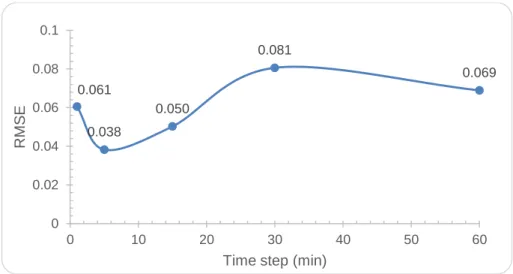
4.2. Case 1 - Selection of the time step ... 39

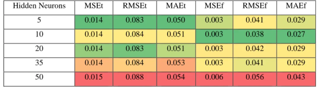
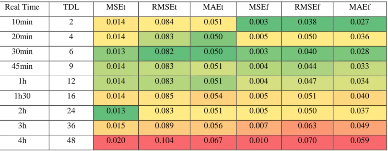
4.3. Case 2 - NARX network with data of 4 PV systems as exogenous inputs. ... 40

4.4. Case 3 - NARX network with data of 2 PV systems as exogenous inputs ... 44

4.5. Case 4 - NARX network with data of 2 meteorological parameters as exogenous inputs.50 4.6. Case 5 - NARX network with 4PV systems and meteorological data as exogenous inputs. 53 4.7. Best neural network configurations from Case 2 to 5 ... 59

4.8. Case 6 - Multistep ahead forecasting ... 60

5. CONCLUSION ... 65

6. REFERENCES ... 67

(8)

viii

Figure 1 - Relation between forecasting horizons, forecasting models and the related activities.

(Diagne, David, & Boland, 2012) ... 3

Figure 2 - Classification of the forecasting models (Temporal Resolution vs Spatial Resolution). (Diagne et al., 2012) ... 4

Figure 3 - Biologic and artificial neuron designs. (Krenker, Bešte, & Kos, 2011) ... 5

Figure 4 - Single-Input Neuron. (Beale, Hagan, & Demuth, 2013) ... 6

Figure 5 - Neuron with vector input. (Beale et al., 2013) ... 6

Figure 6 - Feedfoward neural network with n inputs, a layer of Nc hidden neurons, and N0 output neurons. (Krenker et al., 2011) ... 8

Figure 7 - Multilayer artificial neural network. (Krenker et al., 2011) ... 9

Figure 8 - Fully recurrent artificial neural network. (Krenker et al., 2011) ... 10

Figure 9 - Nonlinear autoregressive with exogenous inputs (NARX) model. (Haylin, 1999) ... 12

Figure 10 - Overtraining example. (Palit & Popovic, 2005) ... 14

Figure 11 - Early stopping of training. (Palit & Popovic, 2005) ... 14

Figure 12 - Steepest descent method with different learning constants. The trajectory on the left is for small learning constant that leads to slow convergence; the trajectory on the right is for large learning constant that causes oscillation (divergence). (Yu & Wilamowski, 2010) ... 16

Figure 13 - Light incident on the cell creates electron-hole pairs, which are separated by the potential barrier, creating a voltage that drives a current through an external circuit. (Zweibel, 1982) ... 21

Figure 14 - Schematic of a grid-connected photovoltaic system. (Twidell & Weir, 2006) ... 22

Figure 15 - Grid-connected system functioning. (Boxwell, 2013) ... 23

Figure 16 - Map of Utrecht illustrating the distribution of the PV systems. ... 30

Figure 17 - NARX network architecture variations. (Beale et al., 2013) ... 33

Figure 18 - Raw time series generated by the PV Systems in the month of July. ... 37

Figure 19 - Meteorological raw data in the month of July. ... 38

Figure 20 - Preprocessing of time series data generated by the Centre PV system. ... 38

Figure 21 - Normalization and interpolation of the meteorological time series. ... 39

Figure 22 - Case 1 RMSE results for the forecasting process using different time steps. ... 40

Figure 23 - Case 2 RMSE results for the forecasting process using different hidden neurons. ... 42

Figure 24 - Case 2 RMSE results for the forecasting process using different TDL. ... 44

Figure 25 - Case 3.1 RMSE results for the forecasting process using different hidden neurons. ... 45

Figure 26 - Case 3.1 RMSE results for the forecasting process using different TDL. ... 47

Figure 27 - Case 3.2 RMSE results for the forecasting process using different hidden neurons. ... 48

Figure 28 - Case 3.2 RMSE results for the forecasting process using different TDL. ... 49

Figure 29 - Case 4 RMSE results for the forecasting process using different hidden neurons. ... 51

Figure 30 - Case 4 RMSE results for the forecasting process using different TDL. ... 52

Figure 31 - Case 5 RMSE results for the foecasting process using different hidden neurons. ... 54

Figure 32 - Case 5 RMSE results for the predicting process using different TDL. ... 55

Figure 33 - Prediction of the last day of the month, using NARX network with 4PV systems and meteorological data as exogenous inputs. ... 56

(9)

ix

the month. ... 57 Figure 35 - Error autocorrelation function. ... 58 Figure 36 - Input-error cross-correlation. ... 58 Figure 37 - Comparison between the optimized networks configurations achieved in each case. The

x label illustrates the input data used in the NARX network. ... 59

Figure 38 - Comparison between the persistence model and the NARX model RMSEf results of anticipating the predictions. ... 62

(10)

x

Table 1 - Characteristics of Algorithms. ... 20

Table 2 - Solar Forecasting - State of the art. ... 27

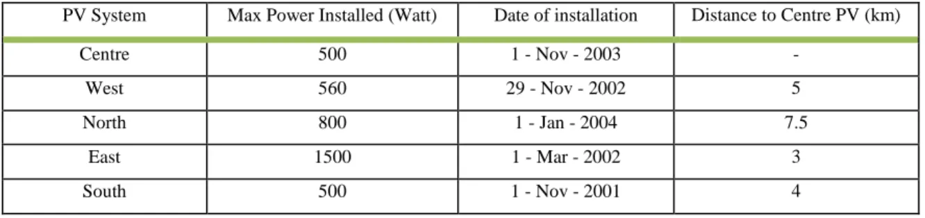
Table 3 - PV systems technical information. ... 29

Table 4 - Case 1 configuration. ... 34

Table 9 - Training and predicting error results using different time steps. ... 39

Table 10 - Training and predicting coefficients of variation using different time steps. ... 39

Table 11 - Case 2 training and predicting error results, using different hidden neurons. ... 41

Table 12 - Case 2 training and predicting coefficients of variation, using different hidden neurons. ... 41

Table 13 - Case 2 training and predicting error results, using different TDL. ... 42

Table 14 - Case 2, training and predicting coefficients of variation, using different TDL. ... 43

Table 15 - Case 3.1 training and predicting error results, using different hidden neurons. ... 45

Table 16 - Case 3.1 training and predicting coefficients of variation, using different hidden neurons. ... 45

Table 17 - Case 3.1 training and predicting error results, using different TDL. ... 46

Table 18 - Case 3.1 training and predicting coefficients of variation, using different TDL. ... 46

Table 19 - Case 3.2 training and predicting error results, using different hidden neurons. ... 47

Table 20 - Case 3.2 training and predicting coefficients of variation, using different hidden neurons. ... 48

Table 21 - Case 3.2 training and predicting error results, using different TDL. ... 48

Table 22 - Case 3.2 training and predicting coefficients of variation, using different TDL. ... 49

Table 24 - Case 4 training and predicting coefficients of variation, using different hidden neurons. ... 50

Table 26 - Case 4 training and predicting coefficients of variation, using different TDL. ... 52

Table 30 - Case 5 training and predicting coefficients of variation, using different TDL. ... 55

Table 31 - Comparison between the best network configurations achieved in each case. ... 59

Table 32 - Error results of anticipating the predictions using the NARX model. ... 61

Table 33 - CV results of anticipating the predictions with different intervals. ... 61

(11)

xi

AC Alternating current

ACF Autocorrelation function

AIC Akaike’s information criterion

ANN Artificial neural network

AR Autoregressive

ARIMA Autoregressive Integrated Moving Average

ARMA Autoregressive Moving Average

BIC Bayes information criterion

CPV Concentrated Photovoltaic

CSP Concentrated Solar Power

CV Coefficient of Variation

DC Direct Current

EBP Error Backpropagation

GHG Greenhouse Gas

KNMI Royal Netherlands Meteorological Institute

MA Moving Average

MAE Mean Absolute Error

MLP Multilayer Perceptron

MSE Mean Squared Error

NAN Not A Number

NARX Nonlinear Autoregressive with eXogenous

NWP Numerical Weather Prediction

PACF Partial Autocorrelation Function

PV Photovoltaic

RMSE Root Mean Squared Error

SSE Sum Squared Error

TDL Tapped Delay Line

(12)

André Gabriel Casaca de Rocha Vaz 1

1. INTRODUCTION

1.1. Introduction

The world’s electricity consumption is growing exponentially as a consequence of world population growth and increasing per capita demand. As a result, primary energy demand will increase and, without appropriate measures, an increase in energy related greenhouse gas (GHG) emissions is expected with severe effects on our climate. However, there are development paths that allow GHG concentrations to stabilize, such as the replacement of fossil fuels (whose reserves are being rapidly depleted) by renewable energy resources, for instance, solar power. Thus, not only a decrease of the GHG emissions but also a reduction of the energy dependence is possible to establish (Heimo, Sempreviva, Kuik, Gryning, 2012).

Nowadays, electrical grids are mostly centralized, transferring power between big power plants towards end users; however, decentralized production units are expected to increase significantly. Approaches to increase electricity transfers amongst grids at different levels and penetration of renewable energies may provide a more efficient grid management. The challenge for electrical grid operators is to synchronize, continuously, the demand with energy supply.

Accordingly, as global demand for renewable energy is increasing, the economic and technical issues of solar power penetrations into the power grid must be addressed. The flat-panel PV, Concentrated Solar Power (CSP), and concentrated PV (CPV) systems are considered the most liable sources of solar energy technology to compete with fossil fuel energy production in the near future. However, natural variability of the solar resource, seasonal deviations in production and the high cost of energy storage raises concerns regarding reliability and feasibility of these systems. Moreover, solar plants usually have the support of generators for periods of high variability, increasing the costs with personnel and financially (Inman, Pedro, & Coimbra, 2013).

Unlike conventional power sources, future electricity supply cannot be precisely planned beforehand. This is due to the fact that solar energy is highly dependent on weather conditions especially cloud structure and day/night cycles. Clouds can cause significant ramps in solar insolation and PV output. Therefore, integration of electricity produced by solar power systems requires accurate solar energy potential availability evaluation and several time horizons forecasts because electricity generation varies in time and, hence, energy production pattern does not always follow the load demand. To successfully integrate increased levels of solar power production while maintaining reliability is the biggest challenge for solar energy supply and makes the availability of accurate information an important necessity.

Solar forecasts on multiple time horizons play a fundamental role in storage management of PV systems, control systems in buildings, control of solar thermal power plants, as well as for the grids’ regulation and power scheduling. It allows grid operators to adapt the load in order to optimize the energy transport, allocate the needed balance energy from other sources if no solar energy is available, plan maintenance activities at the production sites and take necessary measures to protect the production from extreme events.

Depending on the purpose, different sorts of information are needed, such as the long term historical data sets of the expected energy yield (in order to assess sites where solar power systems can possible be implemented), real-time data sets (supports and optimizes energy production management), forecasted site irradiances (supports regional power grids management), local solar resource characterization and reliable estimates on the availability of solar irradiance (to uphold socio-economic planning) and, finally, real-time datasets on weather conditions (supporting forecasting of electricity demand, since this is essential to determine prices and trading of electric power) (Espinar, Aznarte, Girard, Moussa & Kariniotakis, 2010).

(13)

1.2. Motivation and Goals

Accurate solar forecasting methods improve the quality of the energy delivered to the grid and reduce the additional cost associated with weather dependency. The combination of these two factors has been the main motivation behind several research activities.

Although the existent solar forecast systems remain evasive, several approaches that combine atmospheric physics, solar instrumentation, machine learning, forecasting theory and remote sensing have been developed and presented promising results in the solar energy meteorology field. A recent study regarding a power forecasting system designed to optimize the scheduling of a small energy network including PV is described in (Kudo, Takeuchi, Nozaki, End, & Sumita, 2009). Using advanced communication networks and power predictions, the electric power and heat may be controlled especially for optimizing the energy flow. Also, a different study (Rikos, Tselepis, Hoyer-Klick, & Schroedter-Homscheidt, 2008) shows the influence of weather disturbances on the stability of an island micro-grid power system. They described how the stability may be improved when information on cloud cover approaching the island is available 15 minutes in advance. They also conclude that this information allows the start-up of power backup or the disconnection of less critical loads.

Some methods behave better for shorter time horizons and others perform better for longer time horizons. Usually, the time horizon is divided in long-term (6 hours up to days ahead) and short-term (up to 6 hours ahead). The day-ahead forecasts are required by about noon for each hour of the next day, whereas, for example in California, the intra-day ahead forecasts have to be submitted 105 minutes prior to each operating hour and at the same time have to provide advisory forecasts for the 7 hours after the operating hour (Pelland, Remund, Kleissl, Oozeki, De & Brabandere, 2013). Numerical weather forecasts, times series approaches, neural networks, use of satellite and total sky images are amongst the most used methodologies.

Numerical weather forecasts (NWP) are a common strategy for long time horizons of more than 6 hours forecasts. Basically, NWP predicts the weather by using current conditions as input into mathematical models and it has been used to forecast solar irradiance for up to several days in (Hammer, Heinemann, Hoyer-Klick, Lorenz, Mayer, & Schroedter-Homscheidt, 2007), (Lorenz, Hurka, Karampela, Beyer, & Schneider, 2008) and (Remund, Perez, & Lorenz, 2008). However, this model does not have the spatial or temporal resolution for a detailed mapping of small scale features and cannot predict how a certain solar panel is affected by cloud fields.

However, there are also classic approaches, as the times series approach, that traditionally forecast solar energy based on the time series of weather conditions and solar energy. Regarding long-term forecasting, the models used in (Bie & Musikowski, 2008), (Brinkworth, 1977) and (Puri, 1978) are based on weather station data and climate time series. On the other hand, for a time scale smaller than a day, information about cloud cover is necessary. In (Bacher, Madsen, Nielsen, & Plads, 2009) and (Dazhi, Jirutitijaroen, & Walsh, 2012) Autoregressive Models (AR), Moving Averages (MA) and Autoregressive Models Moving Averages (ARMA) are used to model linear dynamics structures and forecast hourly solar irradiance times series using cloud index.

Given the limitations of the basic models previously presented, research has been done in nonlinear models that show more flexibility in capturing the data underlying characteristics (Artificial Neural Networks). In order to fit the network, training of the model is involved over the known input and output values. The authors in (Zeng & Qiao, 2011) show that an artificial neural network-based model for short-term solar power prediction outperforms the AR model.

(14)

André Gabriel Casaca de Rocha Vaz 3 The use of total sky and satellite images stand out as models for very short-term forecasting because incorporate information on the actual atmospherics state by applying image processing and cloud tracking techniques. In (Jayadevan, Rodriguez, Lonij, & Cronin, 2012) the authors analyzed digital images taken with a ground-based sun tracking camera and discuss statistics of ramp rates and duration of cloud induced intermittencies; Also, (Marquez & Coimbra, 2012) describes several sky image processing techniques relevant to solar forecasting, including velocity field calculations, spatial transformation of the images, and cloud classification.

Furthermore, satellite imagery is based on the premise that clouds reflect light from earth into the satellite, leading to the detection and ability to calculate the amount of light transmitted. The low spatial and temporal resolution causes satellite forecasts to be less accurate than total sky imagery. However, in the 1 to 5 hours range satellite imagery has a better forecasting accuracy. In (Hoff & Perez, 2012), the authors suggested that satellite-based irradiance has an annual error comparable to ground sensors and is suitable to provide the data required to perform high penetration PV studies.

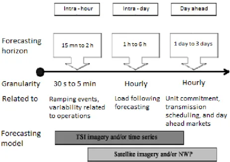
As illustrated in Figure 1, for the very short-term time horizon, from minutes up to a few hours, time series models using on-site irradiance measurements or power data as input are adequate. Moreover, regarding Intra-hour forecasts of clouds and irradiance with a high spatial and temporal resolution total sky images are the best option. Forecasts based on cloud motion vectors from satellite images show good performance for a temporal range of 30 minutes to 6 hours. Finally, grid integration of PV power mainly requires forecasts up to 2 days ahead or even beyond and these forecasts are based on NWP models.

Figure 1 - Relation between forecasting horizons, forecasting models and the related activities. (Diagne, David, & Boland, 2012)

(15)

André Gabriel Casaca de Rocha Vaz 4 Figure 1 depicts the temporal and spatial resolution of different forecasting models. ARIMA models present significant reliability in the statistical forecasting model range. However, one verifies in Figure 2 that the persistence1 model often achieves better accuracy than ARIMA-type models for real time forecasts. The choice of the model depends critically on the horizon of forecast. At higher frequency, short-term patterns dominate and Artificial Neural Networks demonstrated good results. (Diagne e al., 2012)

The present work intends to use an artificial neural network (ANN) model to capture the short-term ramping patterns caused by cloud formations and to forecast a PV system power output up to 1 day ahead. Moreover, using different input combinations, we want to assess whether or not solar power forecasts can be improved by knowing beforehand the power output of other neighbouring grid-connected PV systems and local meteorological information.

1.3. Thesis Scope

In section 2, an introduction to the architecture and relevant variations of neural networks is presented. Furthermore, typical photovoltaic systems are described and the current state of the art of solar forecasting with artificial neural networks is reviewed. Additionally, several functions that can evaluate the quality of the neural network predictions are indicated. Section 3 describes the design and implementation of the NARX model using neural networks. In section 4, the results of the experiments and tests are presented and thoroughly discussed. Finally, in section 5, the conclusion of the work and future research expectations in the solar forecasting domain are elaborated.

1

Simple model that meets the definition: X n,y = X n-k,y where k denotes the lag (k = 1,2,3,..,m).

Figure 2 - Classification of the forecasting models (Temporal Resolution vs Spatial Resolution). (Diagne et al., 2012)

(16)

2. PHOTOVOLTAIC FORECASTING

2.1. Artificial Neural Networks

A thorough understanding of the architecture of neural networks is important to avoid disappointing results and, thus, identify and establish better parameters to improve the network performance. Therefore, this section describes the fundamentals of artificial neural networks.

The design and functionalities of the artificial neuron derive from the observation of the complex biological neuron in which distributed information is processed in parallel by mutual dynamical iterations of the neuron. Accordingly, there are some similarities between the biological neural network and the artificial neural network and one can verify it in Figure 3. In the biological neuron the information comes into the neuron via dendrite, soma processes it and passes it on via axon. Similarly, in the artificial neural network the information comes from the inputs that are weighted. Consequently, in the artificial neural body the weighted inputs and bias are summed and processed with a transfer function. After being processed, the information is passed via outputs.

Different learning rules can be chosen and applied, and, consequently, the weights and bias are adjustable parameters so that the neuron input/output achieves a specific end. In any artificial neural network model, it is important to consider the structure of the nodes, topology of the network and the learning algorithm. Therefore a broader view of the mathematical and fundamentals and algorithms will be presented.

2.1.1. Artificial Neural Networks: Definitions and Properties

2.1.1.1. Single Input-Neuron

A neural network consists of simple processing units, the neuron, and directed, weighted connections between those neurons (Figure 4). The inputs channels have an associated weight, which means that the incoming information is multiplied by the corresponding weight . The network input is the result of the latter process, so-called propagation function. Here, the strength of a connection between two neurons and is a connecting weight and illustrated by . (Kriesel,

2005)

(17)

André Gabriel Casaca de Rocha Vaz 6 These connecting weights can be inhibitory or excitatory and by being connected with the neurons, data are transferred. Figure 4 illustrates the single-input neuron. is formed after the scalar input is multiplied by the scalar weight . Consequently, , often referred to as the net input is processed into a transfer or activation function . The latter process gives the scalar neuron output . Thus, the output is a function of the particular activation function chosen and the bias. The latter is similar to a weight, albeit it has a constant input of 1. This bias term is used by the neuron to generate an output signal in the absence of input signals.

2.1.1.2. Neuron with vector input

The simple neuron previously shown can be extended to handle inputs that are vectors. The concept is the same as before: the individual elements in a neuron with a single R-element input, vector are multiplied by weights and then fed to the summing

junction. The sum of the weighted values is , the product of the matrix and the vector . In order to form the network input , there is a bias in the neuron which is summed with the weighted inputs. Consequently, the network input n is the argument of the activation function ,

(1)

Figure 4 - Single-Input Neuron. (Beale, Hagan, & Demuth, 2013)

(18)

2.1.1.3. Transfer function

Transfer function or activation function controls the amplitude of the output of the neuron and is based on the neurons reactions to the input values and depends on the level of activity of the neurons (activation state). This premise is founded on the biological model, where every neuron is, at all times, somewhat active. Essentially, neurons are activated when the network input exceeds the uniquely maximum gradient assigned value of the activation function, known as threshold. Accordingly, near the threshold value the activation function has a rather sensitive reaction. The activation function is dependent of the previous activation state of the neuron and the external input and is defined as

( )

(

( )

)

(2)

This equation demonstrates how the network input , previous activation state ( ) and the influence of the threshold , is transformed into a new activation state ( ). It must be

emphasized that though the threshold values are different for each neuron, the activation function embraces all neurons.

Two of the most commonly used activation functions in neural networks are the logistic and hyperbolic tangent function. Both functions are used because of the simplicity in finding its derivatives. Usually, these functions are applied in the hidden layer of the network.

The logistic function, ( ) ₍₎ takes the input with any value between plus and minus infinity and maps the output to the range values (0, 1). The hyperbolic tangent: ( )

also takes the input with any value between plus and minus infinity and squashes

the output into the range -1 to 1. The selection of the activation function provides nonlinear limits to the hidden neurons and influences the performance of the networks. To avoid bad performances, one usually preprocesses the input data, for example, by normalizing the data.

Another relevant function is the linear function ( ) , where the inputs and outputs range from minus infinity to plus infinity, which it is generally used in the output layer of the network.

2.2. Neural Networks Architecture

The neuron is a nonlinear, parameterized function of its input. The configuration of the nonlinear functions of two or more neurons is a neural network. The next sections introduce the different neural networks classes: feedfoward networks and recurrent (feedback) networks.

(19)

2.2.1. Feedforward Neural Networks

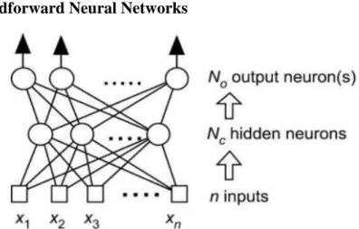
A Feedforward neural network is a nonlinear function of its inputs, which is the composition of the functions of its neurons. As Figure 6 illustrates, the information runs through the connected neurons only in the forward direction, from inputs to outputs. Graphically, the vertices are the neurons and the edges are the connections; these types of networks do not have back-loops. Obviously, the term connection is taken metaphorically because the computations by each neuron are implemented as software programs.

2.2.2. Multilayer Networks

Most neural networks applications require the use of multilayer networks with a similar topology as the one in Figure 6, which illustrates how the network computes N0 functions of the

input variables of the network; each output is a nonlinear function of the nonlinear functions computed by the hidden neurons. In other words, in the Feedforward neural network the nonlinear functions are computed based on the previous computation of the functions computed by the hidden neurons.

Feedforward neural networks are considered static neural networks models, that is, models applicable to processes where the setting for each piece are determined up front, and are not altered for that piece using feedback during the process. (Coit, Jackson, & Smith, 1997)

Furthermore, Feedforward multilayer networks that use sigmoid nonlinearities are also designated as Multilayer Perceptron (MLP) networks. The following equations and Figure 7 present the structure and calculations required to generate outputs of single multilayers Feedforward artificial neural networks.

(

)

(3)

(

)

(4)

Figure 6 - Feedfoward neural network with n inputs, a layer of Nc hidden neurons, and N0

(20)

(

)

(5)

(

)

(6)

(

)

(7)

(

)

(8)

(

)

(9)

[

(

[

]

[

]]

(

[

]

[

]

])

]

(10)

2.2.3. Multilayer Perceptron and the hidden nodes

The Multilayer Perceptron is one of the most important models in the artificial neural networks domain. For prediction purposes, data is presented to the MLP as a sliding window over the time series observations. The task of the MLP is to model the underlying generator of the data during training, so that a valid forecast is made when the trained neural network is subsequently presented with a new input vector value. (Bramer, 2006)

(21)

André Gabriel Casaca de Rocha Vaz 10 The inherent capability of the three-layer network structure to carry out any arbitrary

input-output mapping highly qualifies the MLP networks for efficient time series forecasting. When examples of the observation data are trained, the networks can learn the characteristic features “hidden” in the examples of the collected data and even generalize the knowledge learnt. (Palit & Popovic, 2005)

The hidden layer nodes are fundamental, albeit there is a large controversy regarding the number of nodes and hidden layers that are necessary to guarantee a good network performance. Due to the fact that no theoretical answer exists, heuristics processes are applied and have been generating some rules of thumb depending on the task. Usually, one hidden layer is enough to characterize the task because several hidden layers may generate unwanted complexity to the problem. (Coit et al.,1997)

In general, one should select enough hidden neurons to generate a solution to a task. However, if the group of patterns of input available is not enough, it is not recommended to have an amount of nodes that generates an estimation of the weights that is not trustworthy.

2.2.4. Recurrent Neural Networks

Recurrent Neural Networks are similar to Feedfoward neural networks but with no limitations regarding back-loops, that is, the network exhibits cycles (Figure 8). Therefore, information may be transmitted both forward and backwards. Consequently, an internal state of the network is created displaying a dynamic temporal behaviour. (Krenker et al., 2011)

Given the fact that the output of a neuron cannot be a function of itself but can be a function of past values, these architectures require time to be explicitly taken into consideration. The ordinary framework applied to recurrent networks is the discrete-time system, which is described mathematically by recurrent equations.

These equations are discrete-time equivalents of continuous-time differential equations. Therefore, besides being assigned a parameter as in Feedforward neural networks, a delay is assigned to each connection of a recurrent neural network (this delay can be made equal to zero). Each delay is a numeric value multiple of an elementary time that is considered as a time unit.

(22)

André Gabriel Casaca de Rocha Vaz 11 Essentially, a discrete-time recurrent neural network follows a set of non-linear discrete-time

recurrent equations, not only through the neurons functions configuration but also through the time delays associated to its connections.

2.3. Dynamic Driven Recurrent Networks

Most dynamical systems involve an autonomous part and a part governed by external force that usually is difficult to identify or noisy. Forecasting deals with dynamic models whose inputs and outputs are related through differential equations, or, for discrete-time systems, by recurrent equations. Recurrent networks with global feedback will be discussed, which is relevant for the scope of this thesis. For a thoroughly understanding of recurrent networks with local feedback, (Haylin, 1999) is suggested.

Considering the typical design of the multilayer networks previously shown, applying the global feedback can take a variety of arrangements. Global feedback can either be in a form of output neuron to the input layer or from the hidden neuron to the input layer. Other architectural layouts for recurrent networks exist, for instance, for multilayer networks with more than one hidden layer; however, those are not relevant for the current work and will not be discussed in detail.

Pertinent to this work is the discussion of recurrent networks used as input-output mapping networks. Basically, in this situation, an external input is applied and the recurrent network has a temporary response. Consequently, the recurrent network is considered as dynamically driven recurrent network. This characteristic enables recurrent networks to acquire state representations, which are fundamental for applications such as nonlinear predictions and modelling. In section 2.7, the recent use of neural networks for forecasting purposes is thoroughly discussed.

2.3.1. Input-Output Recurrent Model

The input-Output recurrent model, with a design that follows the typical multilayer perceptron, is illustrated in Figure 9. One can notice that the model has a single input that is applied to a tapped-delay-line (TDL) memory of elements. A delay line tap extracts a signal output from somewhere within the delay line and usually sums with other taps to form an output signal. Moreover, via another TDL memory with q units, the single output is also fed back to the input. Thus, the contents from both TDL memories are fed to the input layer of the multilayer perceptron.

In Figure 9, ( ) denotes the present value of the model input and ( ) corresponds to the value of the model output. Accordingly, one may understand that the output is one time unit ahead of the input. Hence, the present and past values of the input, which are exogenous inputs generated from outside the network, and delayed values of the output, on which the model output is regressed, are the data window of the signal vector applied to the input layer.

This recurrent network described above and shown in Figure 9 is also referred as nonlinear autoregressive with exogenous inputs (NARX) model (Haylin, 1999).

(23)

( ) ( ( ) ( ) ( ) ( ))

(11)

Equation 11 demonstrates the dynamic behaviour of the NARX model, where is a nonlinear function of its arguments. The two delay line memories in the model are generally different, albeit they can have the same size.

2.4. Training a Neural Network

A key aspect in the implementation of artificial neural networks is the training. This process must be well designed so that the network successfully learns a task. However, one should understand that a precise definition of training is difficult to achieve because there is no direct approach on how to do this (Jain & Mao, 1996). This learning process consists in the adjustment of the weights under some learning rules. Essentially, the free parameters from a network are adapted, through a stimulation process. When a group of patterns is presented, the network typically learns

(24)

André Gabriel Casaca de Rocha Vaz 13 the connection weights and the performance is improved by iteratively updating the weights. The

network learns to recognize the pattern inherent to the training signals.

Though the learning process poses some issues, the ability to automatically learn from examples and learn underlying rules, such as the input-output relationships, makes the neural networks more attractive than traditional systems. Theoretically, the network must approach the global minimum of the objective function, that is, the error function will steadily decrease until the minimum error has been reached. If this is achieved, and no further decrease of the error function is necessary, the training process must be stopped. In practice, the network training can require several training trials with various initial weight values in order to find this global minimum. After each training run, an evaluation and comparison between the training results and the results achieved in the previous run allow us to select the best run.

The design of the training or learning process has to consider the model of the environment in which a neural network works. Thus, one has to distinguish which information is available to the network. Moreover, it is essential to understand how the network weights are updated, i.e. the learning rules that the updating process must follow.

There is not a unique algorithm for the design of neural networks and the learning process of the neural networks can either be classified as supervised or unsupervised training. Essentially, these classifications differ in the existence or not of an external agent (supervisor) that controls the learning process in the network.Other classification criteria reside in defining if the network learns through its normal functioning (online) or if the learning assumes the unplugging of the network (offline). For an online training the weights vary dynamically when new information is shown to the system. Inversely, the networks that use offline learning have their connection weights remain fixed after the training stage.

In supervised training, for every input pattern an output is provided to the network and the external agent controls the answer that the network must generate based on a determined answer, that is, the supervisor compares the output of the network with the expected results and determines the amount of modification that must be applied in the weight. Accordingly, weights are determined so that the result is as close as possible to the known correct answers, i.e. the objective is to find the minimum value of the difference between the answer of the network and the correct answer.

Differently, the unsupervised training organizes patterns into categories from the underlying structure in the data or correlation between patterns in the data. With this method, the neural network is capable of self-organize because there is no information received from the environment indicating the correctness of a generated output. Basically, there is no correct answer required. The interpretation of the output of unsupervised networks depends on the structure of the network and the learning algorithm used. Sometimes the output represents the degree of similarity between the signal introduced in the network and the displayed information until then. Under certain circumstances, grouping of information (clustering) is established, where each category is set based on the correlation between the presented information.

Theoretically, there are some fundamental issues associated with learning from samples that must be considered, such as, the capacity, sample and computational complexity. The capacity refers to the functions and boundaries a network can form, that is, the quantity of patterns that may be stored. Assessing the complexity of the sample is highly important, as it determines the necessary patterns that need to be train in order to achieve a valid generalization. Finally, the computer complexity refers to the time that a chosen algorithm requires to reach an estimate solution from the trained patterns.

(25)

André Gabriel Casaca de Rocha Vaz 14 The experiment design for network training involves concerns regarding the network

initialization training, selection of the appropriate training algorithm, formulation of training stopping criteria, etc.

2.4.1. Avoiding Overfitting

One must find the information that allows us to confirm that the maximum generalization has been reached. Figure 10 presents the case where after reaching the point of maximum generalization the network keeps learning from the training set; however, it starts to damage the related test set performance due to its overtraining. Furthermore, in Figure 10 the overfitting is caused when the validation error increases while training error decreases progressively. Reducing the number of hidden neurons is an option to avoid overfitting. (Tan, 2009)

However, in (Palit & Popovic, 2005) a better approach to solve the training termination problem based on stopping criteria was presented. They developed an automated stopping principle using a predetermined number of training steps. Ideally, the stopping strategy is the one that stops the training after the network has learnt all the problem details it has to solve. Consequently, when the training stopping achieves that stage, the network reaches the maximum generalization. Thus, the minimum value has been reached and this is the point where stopping should be activated. This action is known as early stopping. Beyond this point, the network would be performing the so-called network overtraining or overfitting.

Figure 10 - Overtraining example. (Palit & Popovic, 2005)

(26)

André Gabriel Casaca de Rocha Vaz 15 To prevent overfitting, in (Prechelt, 1998) the author suggested the method of early

stopping with cross-validation. This method proposes the division of collected data into a training set and a test set, and for further partitioning of the training set into the estimation set and validation set. Yet, finding the exact location of the early stopping is not an easy task. Therefore, to manage the problem a stopping principle was introduced consisting in subdividing the training set into the training error Etrain (average error per example across the training set), the test and the validation

error, Etest and Eval respectively.

Both the problem of overfitting and the opposite problem of underfitting are consequences of improper training stopping. The network ability to generalize is affected and lowered by both problems and should be prevented. In the underfitting problem, the network trained is less complex than the task to be learnt, therefore, poorly identifies the structures within a large training data set. Inversely, when trained, a very complex network not only can extract the structures within the training set, it also extracts the embedded noise. This may pose results and predictions that are not acceptable.

The network complexity is related to the number of weights and it is determined by the prediction accuracy of the model selected. The latter depends on the number and size of weights and hidden neurons that would implement the desired prediction accuracy without performing

overfitting. Statistically, the underfitting and overfitting are related to the statistical bias and the

statistical variance they produce. The statistical bias is related to the degree of target function fitting and constrains the network complexity; however, disregards the trained network generalization. The statistical variance (deviation of network learning efficiency within the set of training data) cares about the generalization of the trained network. It is difficult to get the balance between both as the underfitting generates a high bias network and the overfitting produces a large variance.

2.4.2. Training Algorithm

One of the most significant breakthroughs for training neural networks was the development of the steepest descent algorithm, also known as error backpropagation (EBP) algorithm. For each example in the training set, the algorithm calculates the error using a predefined error function, that is, the difference between the actual and desired outputs. After that process, the error is back propagated through the hidden nodes to adjust the weights of the inputs. This procedure is completed when the network converges to a minimum error solution. Though this algorithm is widely used in neural networks, it presents some limitations, in particular slow convergence and easily traps in local minima. (Dreyfus, 2005)

When the gradient is steep, small step sizes should be taken to not rattle out of the required minima. On the other hand, for a small constant step size the training process would be very slow when the gradient is gentle. Also, the classic “error valley” can occur when the curvature of the error surface has different directions and, therefore, can result in slow convergence. However, the slow convergence of the steepest descent method can be significantly enhanced by the Gauss-Newton algorithm which is able to find adequate step sizes for each direction and can converge very fast by using second-derivatives of error function to evaluate the curvature of error surface. Yet, calculating the second-derivatives poses computational complexity.

(27)

André Gabriel Casaca de Rocha Vaz 16 To overcome these problems other learning algorithms were proposed such as the

Levenberg-Marquardt which is suitable for small and medium sized problems and has a fast and stable convergence when compared to other methods. It combines the steepest descent and the Gauss-Newton algorithms. It has the stability of the steepest descent method and the speed of the Gauss-Newton but it is more robust than the Gauss-Newton. The idea is to combine both training processes so that around the area with complex curvature the algorithm switches to the steepest descent algorithm, until the local curvature is adequate to complete a quadratic approximation; later, to speed up the convergence, the algorithm approximately becomes the Gauss-Newton algorithm (Yu & Wilamowski, 2010).

2.4.3. Levenberg-Marquardt Algorithm Origin

This section explains how the Levenberg-Marquardt method derived from the combination of algorithms.

2.4.3.1. Steepest Descent Algorithm

The backpropagation algorithm is used to learn the weights of a multilayer neural network and performs gradient descent to minimize the sum squared error between the network’s output and a certain target value. The error is squared because its magnitude is more relevant than its sign. The total error E is given by the following equation

( )

∑

(12)

where is number of training patters, is the input vector, the weight vector and defines the training error for training pattern . is obtained by,

Figure 12 - Steepest descent method with different learning constants. The trajectory on the left is for small learning constant that leads to slow convergence; the trajectory on the right is for large

(28)

(

)

(13)

where is the network output at the _{output node,}_{is the target output at the} _{output node.}

Every algorithm adjusts the weights and biases to reduce this global error.

To overcome the problem of finding global solutions to the error given the non-linearity of the error function, the algorithm is set to analyze the weight space. Therefore, it is formulated as follows:

(14)

where k is the index of iterations.

The steepest descent algorithm uses the first-order derivative of total error function to find the minima in error space. The first-order derivative of total error function defines gradient :

( )

[

]

(15)

Based on the definition of gradient g, it can be written the update rule of the steepest descent algorithm:

(16)

where α is the learning constant (step size).

All the elements of gradient vector would be very small with a slightly weight adjustment around the solution. Therefore, this training process is asymptotic convergence.

2.4.3.2. Newton’s Method

Newton methods can be relatively slow because they explicitly use the full Hessian matrix

H, which must be calculated and, therefore, some computational expense occurs. The Hessian

matrix H gives the proper evaluation on the change of gradient vector with the second-order derivatives of total error function. Through several mathematical equations and using Taylor Series (Yu & Wilamowski, 2010), it can be demonstrated that:

⇔

(17)

Consequently, the update rule for Newton’s method is

(18)

(29)

[

]

(19)

One is able to identify the differences between the equations of the steepest descent method and the Newton’s method and notice that complementary step sizes are given by the inverted Hessian matrix.

2.4.3.3. Gauss-Newton Algorithm

Although it is rather complicated to calculate the second-order derivatives of the total error function that allow us to determine the Hessian matrix H, this process is essential for Newton’s method because it is applied for the weight updating. To simplify the calculating process, the Jacobian matrix J can be introduced. The Jacobian matrix is the matrix of the first-order partial derivatives of the error function as illustrated in the following equation.

[

]

(20)

The relationship between Jacobian matrix and the gradient vector is shown in (Yu & Wilamowski, 2010) to be

(30)

André Gabriel Casaca de Rocha Vaz 19 where e is the error vector. Moreover, it is proved in (Yu & Wilamowski, 2010) that the relationship

between the Hessian matrix and Jacobian Matrix can be written as

(22)

Consequently,

(

)

(23)

This equation clearly demonstrates that calculating the second-order derivatives of the total error function is not required. Thus, the Gauss-Newton algorithm has this advantage comparing to the standard Newton’s method. Nonetheless, the Gauss-Newton method still presents some problems regarding the convergence for complex error space optimization just as the Newton’s method. Mathematically, the can pose a problem because this matrix may not be invertible.

2.4.3.4. Levenberg-Marquardt Algorithm

The Levenberg-Marquardt algorithm presents another approximation to the Hessian matrix in order to make sure that the matrix is invertible:

(24)

where is the combination coefficient (always positive), and is the identity matrix.

This approximation insures that the matrix H is always invertible because the elements of the main diagonal of the approximated Hessian matrix are larger than zero. Consequently, by combining equation (18) and equation (24), the update rule of Levenberg-Marquardt algorithm is

(

)

(25)

Hence it is demonstrated the combination between the Gauss-Newton algorithm and the steepest descent algorithm. The Levenberg-Marquardt algorithm switches between both algorithms during the training process. When is very small, that is, very close to zero, the Levenberg-Marquardt algorithm switches to the Gauss-Newton algorithm. On the other hand, when is large, the steepest descent method is used because the equation (25) approximates the equation (16). Table 1 summarizes the differences between the different training algorithms and its main features regarding speed, stability and computational complexity.

(31)

André Gabriel Casaca de Rocha Vaz 20 Table 1 - Characteristics of the algorithms.

Algorithms Update Rules Convergence Computational

Complexity

EBP Stable, slow Gradient

Newton

Unstable, fast Gradient and Hessian

Gauss-Newton ( )

Unstable, fast Jacobian

Levenberg-Marquardt

( )

Stable, fast Jacobian

One might have noticed that according to the updating rule of the Levenberg-Marquardt algorithm, if the error is decreasing, that is, the error in is smaller than in the coefficient can be reduced so that the influence of gradient descent part is diminished. However, if the opposite occurs, if the error increases, it is necessary to follow the gradient to look for a proper curvature for quadratic approximation and the coefficient is increased.

The main drawback of the Levenberg-Marquardt algorithm is that it requires the storage of some matrices that can be rather large for certain problems.

The following section introduces the photovoltaic technology and further down the use of artificial neural networks in the photovoltaic domain is discussed.

2.5. Photovoltaic Systems

The sun can be considered as the source of almost all energy on the planet, because most of the available energy is directly (sunlight) or indirectly (wind and waves) related with it. The sun’s apparently ability to provide endless energy results from the process of nuclear fusion. This energy, produced in the core of the sun, is emitted as electromagnetic radiation. Though electromagnetic radiation is emitted in many useful forms, the solar cell designers are more interested in capturing the energy carried in visible light. (Stapleton & Neill, 2012)

The present section introduces typical small-scale PV systems from which information regarding the systems’ energy production is collected. This section also analyses relevant factors that influence that production.

2.5.1. Photovoltaic Technology

PV cells are devices that produce electricity directly from electromagnetism radiation. These devices are made from semiconducting materials, which conduct electricity under specific conditions, so they are neither insulators nor conductors. The most common semiconductor material is silicon, which is often combined with other elements to improve its conductivity, in a process

(32)

André Gabriel Casaca de Rocha Vaz 21 designated as doping. Controlled quantities of specific impurity ions are added to the very pure

material to produced doped semiconductors.

Impurity dopant ions of fewer valences (e.g. boron) enter the solid Si lattice and become electron acceptor sites which trap free electrons. These traps have an energy level within the band gap, but near to the valence band. The absence of the free electrons produces positively charged states called holes that move through the material as free carriers. With such electron acceptor impurity ions, the semiconductor is called p (positive) type material, having holes as majority carriers. On the other hand, atoms of great valency (e.g. phosphorus) are electron donors, producing n (negative) type material with an excess of conductions electrons as the majority carriers. (Twidell & Weir, 2006)

An electron free to move throughout the crystal is said to be in the crystal's conduction band, because free electrons are the means by which electricity flows. Both the conduction-band electrons and the holes are fundamental in the electrical behavior of PV cells. Although the generation of electrons and holes by light is the central process in the overall PV effect, it does not itself produce a current.

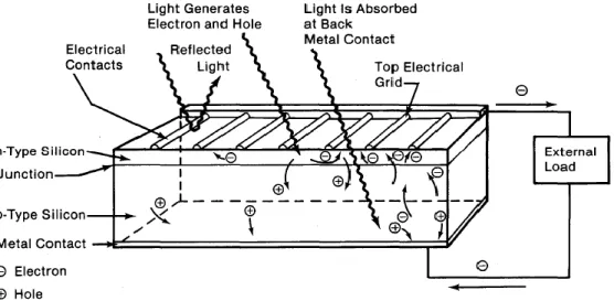
A PV cell contains a barrier that is set up by opposite electric charges facing one another on either side of the junction. This potential barrier selectively separates light-generated electrons and holes, sending more electrons to one side of the cell, and more holes to the other. This charge separation sets up a voltage difference between either ends of the cell, which can be used to drive an electric current in an external circuit. (Zweibel, 1982)

If we connect the n-type side to the p-type side of the cell by means of an external electric circuit, current flows through the circuit because this reduces the light induced charge imbalance in the cell. This current from the cell is inherently direct current (DC). Figure 13 illustrates the functioning of a typical PV cell.

Figure 13 - Light incident on the cell creates electron-hole pairs, which are separated by the potential barrier, creating a voltage that drives a current through an external circuit. (Zweibel, 1982)

(33)

2.5.2. Grid-connected PV systems

PV cells are used to create PV modules that can then be used to create a PV array, which is the principal component of a grid-connected PV system.

Although small-scale PV systems may be applied in many different ways, the residential grid-connected PV systems are the most relevant configuration for this thesis scope. In these systems, any surplus of energy being produced is fed into the grid. Figure 14 and Figure 15 illustrate the functioning of the PV system and the required basic structures (PV array, Inverters, metering, controllers, and electrical devices) that allow an effective and safe interaction with the power grid. These are merely illustrative designs and variations are most likely possible.

Given the fact that a PV system generates electricity as DC and the one coming from the grid is alternating current (AC), an inverter is required to convert DC power from the PV array into AC power to be used by appliances on site or fed back into the grid via the meter. This conversion is possible due to the inverter’s switching mechanism that allows the circuit to rapidly open and close. (Boxwell, 2013)

The grid-connected PV system uses grid-interactive inverters, also known as grid-tied inverters, which are crucial for the transfer of the electricity produced by a PV system into the grid. The grid-interactive inverter finds the maximum power available from the PV array to convert to AC and ensures that the power being fed into the grid is at the appropriate frequency and voltage. Most grid-interactive inverters include transformers that are used to increase the voltage to the level required by the grid.

When the grid is not operating within adequate voltage and frequency tolerances, the inverter has active and passive safety protections that allow shutting itself down. The inverter’s ability to detect the grid’s voltage and frequency is known as passive protection, whereas active protections is provided by the inverter detecting any frequency instability, frequency shift or power variation that would vary the voltage that the inverter detects. Moreover, the grid-connected inverter detects power cuts and monitors the power feed from the grid and if any extreme conditions occur it will disconnect, protecting not only the grid but also the PV system. Additionally, the amount of energy taken from the grid and fed back into the grid is monitored by the grid-connected meter. (Stapleton & Neill, 2012)

Other components involved in the PV system functioning are known collective as the balance of system (BoS) equipment and often must comply with local and/or national codes and regulations. These components are required to connect and protect the PV array and the inverter and includes cabling, disconnects/isolators, protection devices and monitoring equipment. (Stapleton & Neill, 2012)