Equity valuation using accounting numbers : research question : effects of R&D intensity

(1)

Equity Valuation Using Accounting Numbers

Research Question – Effects of R&D Intensity

Author – João Santos Marques

Advisor – Geraldo Cerqueiro

Dissertation submitted in partial fulfilment of requirements for the degree of MSc in Business Administration at Católica Lisbon School of Business and Economics, 16th September 2013

(2)

(3)

3

Abstract

Recent studies have been studying effects of R&D intensity in equity valuation, e.g. by analyzing the telecommunication industry, Amir and Lev (1996) conclude accounting numbers to be useless for this purpose. As a consequence, literature has been raising the question of whether R&D expenses are properly priced and represented in the main valuation methods adopted by analysts. This dissertation pretends to approach this question by establishing and testing 8 hypotheses for two different samples, a large and a small. The intention is to alert the user about how methodologies for equity valuation vary within different levels of R&D intensity.

Empirical results suggest that R&D intensity tend to deteriorate models’ performance, being the Price Earnings Ratio the most effective. On the other hand, empirical results suggest analysts to ignore performance effects of R&D intensity when valuing firms as there are no differences in their preference for valuation models between the two groups. Moreover, there is no significant difference between analysts’ pattern of recommendation (considering ‘buy’ and ‘sell’ against ‘hold’). Finally, despite drawbacks of cash flows figures when compared to earnings, there is evidence of analysts’ reliance on it when using flow based valuation models.

(4)

4

1. Introduction

Prior studies have been studying effects of R&D intensity in equity valuation, e.g. by analyzing the telecommunication industry, Amir and Lev (1996) conclude accounting numbers to be useless for this purpose. As a consequence, literature has been raising the question of whether R&D expenses are properly priced and represented in the main valuation methods adopted by analysts.

This research pretends to approach this question by establishing and testing hypotheses for two different samples. The intention is to alert users about how methodologies for equity valuation vary within different levels of R&D intensity.

A large sample analysis divides between high and low R&D intensive groups within five different industries and follows the methodology of Penman and Sougiannis (1998) and Francis et al (2000) to establish hypothesis about models’ performance (i.e. in terms of bias, accuracy and explanatory power).

On the other hand, a small sample analysis (data hand collected) aims to corroborate or not large sample analysis’ results by outlining how analysts value companies in practice (i.e. which models they use to consider R&D intensity). In this sample, two groups are designed according to R&D intensity.

Generally, this study is divided into three main parts. The first (chapter 2) aims to briefly overview and discuss main literature. Hypotheses defined in later chapters ground on these conclusions. The third and fourth chapters define hypotheses and empirically study them for large and small samples.

(7)

7

2. Review of Relevant Literature

The first chapter intends to briefly overview and discusses main literature regarding: equity valuation foundations and its grounds (section 2.1 and 2.2); theoretical valuation models and empirical evidence about it (section 2.3); empirical evidence on Research & Development intensity (section 2.4). The intention is to provide user to main background of further statistical analysis, which will consist on equity valuation with a particular scope on firms’ Research & Development intensity.

2.1. Foundations of Equity Valuation

This section intends to highlight the relevance of accounting numbers for Equity Valuation. Firstly, the concept of Equity Valuation must be clarified. For Lee (1999) it is as much as an art as it is a science, what can also be referred as a subjective task that requires an ‘educated guess’ to look into an uncertain future, and transform forecasts into key value estimates (Penman, 2008).  

The valuation process is crucial to any business and agents of every industry regardless of being external or internal. Not only managers and shareholders need it to make strategic decisions regarding capital structure (e.g. Debt issuance) and company’s operations (e.g. capital budgeting and project viability analysis), but also external analysts use it as a powerful tool to perform their activity, namely to provide potential investors with fair values of target companies (Palepu et al, 1999).  

The Equity Valuation process is sometimes underestimated because stock prices, assuming that markets are efficient, instantly provide companies’ intrinsic values. Nevertheless, in some cases, share price may not be fully informational. Firstly, private companies are not quoted on financial markets and Equity Valuation appears as a solution to provide fair value in case of an M&A or an IPO. Secondly, assuming that market efficiency may not imply that companies are correctly priced (Damodaran, 2002), and that Equity Valuation serves as a tool to check and correct for mispricing. Finally, firm’s intrinsic value is just the final output of a long process called Equity Valuation, which, all through it, produces useful information that share price cannot provide, for all agents interested on it. 

(8)

8 2.2. Usefulness of Accounting Numbers

The essential task of Equity Valuation is forecasting. It is this process that ‘breathes life’ to valuation and is driven by fundamental analysis that consists on the ‘art of using existing information’ (Lee, 1999). Despite not directly designed to value businesses, financial reporting is the starting point for forecasting. Relevant figures to forecast are those that are representative of firm’s performance. Net income is seen as the figure that most effectively gathers information about the company. This idea was introduced by Ball and Brown’s (1968) which tested usefulness of earnings, suggesting more than a half of the announced information about a company in a year to be in the net income number. Nearly thirty years later Lee (1999) claimed that ‘earnings are a conceptually defensible and reasonably objective measure of firm performance’.

Nevertheless, in the literature, earnings were not always referred as useful. As a matter of fact, Ball and Brown’s (1968) decided to test the usefulness of earnings as, until then this was considered to be meaningless for some literature. Mentions to this hypothesis are present in the works of Gilman (1939), Paton and Littleton (1940), Edward and Bell (1961), among others. Lev (1989) claims that the ‘intertemporally unstable contemporaneous correlation between stock returns and earnings’ suggesting a limited usefulness of earnings whilst Beaver (1968) advocates this measure to be useful as long as it can change investors’ decisions.

2.3. Valuation Models

2.3.1. Perspectives of Valuation

There are two perspectives on which Valuation Models ground. Some models value firms on the Equity Level and others on the Enterprise Level (also mentioned as Entity Level/Perspective). The first ones value directly the equity value of a company what reflects the company’s market value (Share price if divided by shares outstanding). The second value the company’s assets and reach Equity Value by subtracting Net Debt. Equation 1 illustrates the relationship between Equity and Enterprise and shows that, in theory, if well performed, both perspectives should lead to the same intrinsic value. Palepu et al (2000) analysis suggests that the Discounted Cash Flow Model (Entity Level) and the Residual Income Model (Equity Level) lead to the same valuation figure.

(9)

9 (1) (2) (3) (4)

Enterprise Level models consider all claims (equation 2) in a company, both from owners and debt, whilst Entity Level models only consider owners claims in its valuation (equation 3).

2.3.2. Stock Based Valuation Model

Stock based valuation models or multiples valuation is a popular method for Equity Valuation. It is a simpler and less costly approach when compared with flow based valuation models that requires fundamental analysis. This group of Models distinguishes by not using multi-period forecasts and by using a value driver based on comparable firms.

Equation 4 illustrates the methodology used by Stock Based Valuation Models. First, depending on the type of firm, a relevant value driver must be selected (e.g. earnings, EBITDA). Second, comparable firms must be selected under certain criteria defined by the analyst to compute the benchmark multiple that consists on an average of the peer group. Under this group of models, comparable firms are assumed to have similar risk and value profitability profiles as the target firm. Lastly, this model assumes value driver to be proportional to company’s value.

The intention is to provide the user most popular methodologies of using stock based models as well as some empirical evidence on these types of models.

2.3.2.1. Selection of Relevant Value Driver

(10)

10 more adequate than others. This way, relevant value drivers must represent the figure that most faithfully represents value/price relationship.

Accruals are generally preferable over cash flow figures in order to avoid mismatching and timing problems. Moreover, Liu et al (2002) advocate that amongst accruals earnings is the most accepted figure to use. Nevertheless, equity level multiples are affected by leverage and therefore, a reformulation of the multiple is advised in order to focus on the entity level (Penman 2003). Lastly, the use of forecasted figures is advisable over historical numbers due to its higher informational content. Forecasted figures are likely to represent more accurately market values than book values (Ohlson Juettner-Nauroth, 2005). This way, forward earnings is usually the relevant value driver to use (Liu et al, 2002).

2.3.2.2. Selection of Comparable Firms

An important part of this type of valuation process is the selection of comparable firms to form a peer group. Theoretically, the best comparable firm is one that meets model’s assumptions, namely same risk profile and level of performance and profitability. Despite in reality there are not two equal companies, it is possible to define some criteria to identify comparable companies such as:

(a) SIC codes can be used to identify companies performing on the same industry. (b) Leverage Ratios might be a good proxy of risk profile. (c) Earnings, revenue and cash-flow figures might be a good indicator of profitability. (d) ‘Warrented Multiple’ proposed by Bhojraj and Lee (2002), not only gathering company’s specific characteristics but also the association between the target firm and the economy as a whole

Using SIC codes as the only criteria to select comparable companies might turn out to be a dangerous due to high intra-industry differences (Penman, 2003).

2.3.2.3. Computing the Benchmark Multiple

After defining the relevant value driver and selecting the most adequate comparable firms a benchmark multiple must be computed. Due to its sensitivity, the way of computing it should be

(11)

11 (5)

(6)

(7)

(8) carefully chosen. Different methods can lead to largely different intrinsic values (Liu et al, 2002; Fernandez, 2002). The four most popular methods are represented in equations 5 to 8.

The use of arithmetic average 5) Can be biased by the presence of extreme values (outliers). In fact, Baker and Ruback (1999) argue that the use of this method tends to overvalue companies. The use of weighted average (6) and median (7) diminish this problem. Alternatively, the method that minimizes the most the upward-bias problem is the harmonic mean (8), considered to be the one that produces best valuation performance (Baker and Ruback, 1999).

2.3.2.4. Empirical Evidence on Stock Based Valuation Models

Enterprise multiples are considered to be preferable over Equity Multiples if accounting policies differ. Furthermore, Enterprise Multiples are less affected by capital structure policies and its use is advisable. Nevertheless, analysts are encouraged to adopt Equity Multiples when the use of Entity Multiples does not add relevant information to the analysis in order to avoid additional forecasts. Recent Literature has been studying the usefulness of stock-based valuation models as well as the most appropriate way to use it. Evidence of this research is present in the works of Liu et al (2002), Bhojraj and Lee (2002), Alford (1992) and Lie and Lie (2002). This section will have a particular focus on the first two works.

(12)

12 Liu et al (2002) compared the effectiveness of several multiples when differently specified. The ultimate goal is to determine which value driver performs best when using the most adequate method to compute benchmark multiple and given two approaches to select comparable companies. In this study the two approaches were considered when selecting comparable firms: (i) Traditional approach of selecting all firms of the industry that matches Alford’s (1992) approach that considers 3-Digit SIC codes. (ii) ‘Broader approach that allows for an intercept and examine the effect of expanding the group of comparable firms to include all firms in the cross-section’ (Liu et al, 2002). Furthermore, benchmark multiple was computed using harmonic mean.

The authors’ research leads to two main findings. First, forward earnings are a value driver the value driver that performs better. Second, using companies from the same industry as comparables leads to better results than the alternative method used that underestimates prices.

With a different aim, Bhojraj and Lee (2002) researched about the best way of selecting comparable firms. The analysis was based in two valuation multiples, Enterprise Value/Sales and Price-to-book, in order to avoid negative denominators. The article proposed the use of a ‘warranted multiple’ and compared it with the traditional approach of selecting comparable firms by industry and company’s size. Each firms has a ’warranted multiple’ that is computed in accordance not only to company’s specific characteristics but also the association between the target firm and the economy as a whole. Peer Groups would then be selected according to the similarity of ‘warranted multiple’.

The use of ‘warranted multiple’ to select comparable firms has a higher explanatory power for valuation (i.e. superior ability to predict firm’s value) than the traditional approach of selecting the whole industry (Bhojraj and Lee, 2002). Nevertheless, the traditional approach owes its popularity to its straightforward concept, unlike the approach proposed by the authors which is considered to be more complex.

2.3.3. Flow Based Valuation Models

This section will cover the four main flow based valuation models discussed in literature; Dividends Discount Model, Discounted Cash Flow Model, Residual Income Model and Ohlson

(13)

13 (9)

(10) Juettner-Nauroth Model. Flow based valuation models distinguish from stock based by grounding on multi-period forecasted and on sensitive assumptions. An explicit and a terminal period are then assumed in the computation of these models. Depending on which model is used and on firms’ characteristics different length of explicit periods.

The intention is to provide the user with main assumptions, mathematical formulas, advantages and drawbacks of each one as well as some empirical evidence on these type of models.

2.3.3.1. Dividends Discount Model

The intrinsic value of Equity can be computed by discounting the forecasted cash-flows for Shareholders, i.e. dividends. Williams’ (1938) Dividend Discount Model (hereafter ‘DDM’) proposes to reach company’s value by discounting future dividends at a given cost of equity (hereafter ke) as equation suggests (number). As any other Flow-Based Valuation Model, DDM establish an explicit period, for which forecasts the payout ratio for each year, and a terminal value.

Where represents dividends at year j and ke the cost of equity to compute firm’s intrinsic value ( ; n stands for length of explicit period.

Depending on the target firm, terminal value can be assumed to grow in perpetuity. Gordon Growth Model introduces variable g, representing long-term growth rate of Dividends.

Where stands for dividends for year j , ke firm’s cost of equity and g represents long term growth to compute firm’s intrinsic value ( ; n stands for length of explicit period.

(14)

14 (11) (12) (13)

(14) DDM appears to be straight forward and effective as it considers the main source of value for shareholders, their payout (i.e. dividends). Nevertheless, this model presents important drawback that prevent analysts from using it sometimes. First, not all companies pay dividends and the model only applies for companies that distribute wealth amongst its Shareholders. Apple inc., founded in 1976, did not distributed dividends between 1995 and 2012. Second, Dividend’s policy might be instable, being hard to forecast. Finally, dividends are seen as wealth-distribution instead of wealth-creation. This way, beyond instable, policies can be arbitrary (e.g. Shareholders compensation on a hostile bid) and not linked to company’s value creation.

2.3.3.2. Discounted Cash-Flow Model

The Discounted Cash Flow Model (hereafter DCFM) is focused on the enterprise level. It values company’s assets by discounting Free Cash Flows to the Firm by the weighted average cost of capital. The intrinsic value is then computed by subtracting Net Debt to the Enterprise Value. There are different methods of estimating Free Cash Flows using published financial statements and all should lead to the same result (see equations 11 to 13).

Where stands for Earnings Before Interests and Taxes; for tax rate; for depreciations; for variation in net working capital; for capital expenditures; for operational cash flow; for cash flow from investments; for operational income; for net operating assets; and for free cash flow; all figures for year j.

The Weighted Average Cost of Capital is computed by the following equation:

Where stands for the Weighted Average Cost of Capital; for tax rate; for cost of equity; for market value of Debt; and for market value of Equity.

(15)

15 (15)

(16) The intrinsic value is then computed by discounting free cash flows at the weighted average cost of capital and removing market value of debt. Note that, like DDM, DCFM also assumes an explicit period and a terminal value (see equation 15 for model with no long term growth rate and equation 16 for model considering long term growth rate).

Where stands for free cash flow for the firm at year j ; for firm’s weighted average cost of capital; for market value of debt; and g represents long term growth to compute firm’s intrinsic value ( ; n stands for length of

explicit period.

This Model enjoys of wide popularity as it is of straightforward application and Cash Flow is an easy concept to think about, not affected by accruals. The major advantage over the Dividends Discount Model is that it applies to any firms, regardless the payout ratio. On the other hand, this model only accounts value creation coming from Cash Flows and treats investments as value losses. This way, the lower is the investment level the higher the company’s intrinsic value. Furthermore, this model requires analysts to adopt long forecast horizons as it uses Cash Flow that are not accrual data and does not recognize value creation in the short-term. Finally, analysts forecast earnings that are based on accrual accounting unlike Cash Flows.

2.3.3.3. Residual Income Valuation Model

The Residual Income Valuation Model (hereafter RIVM) is a derivation of DDM. Nevertheless, it can also value company’s intrinsic value on the entity perspective by avoiding the use of per share data. RIVM defines Residual Income (hereafter RI) as the excess earnings of normal return of Book Value of Equity (O’Hanlon, 2002), with:

(16)

16 (17)

(18)

(19)

Where stands for net income for year j; for book value of equity at year j-1 ; for cost of equity; and for residual income for year j.

RI is positive if Return on Common Equity exceeds cost of equity and negative otherwise. Ohlson (2005) defines it as a premium over the book value. In this model intrinsic value of Equity is computed by the sum of current book value of equity and the forecasted RI’s value discounted at cost of equity. The difference between equations 18 and 19 is that the second presents RIVM expression considering a long term growth rate.

Where stands for residual income for the firm for year j ; for firm’s cost of equity; for book value of equity at time zero; and g represents long term growth to compute firm’s intrinsic value ( ; n stands for length of explicit

period.

RIVM enjoys of some advantages over other models. Unlike DCFM, it is based on earnings that use the proprieties of accrual accounting, matching value added with value given up, and considers investment as value creation instead of value loss. This way, this model requires a shorter forecast horizon.

RIVM owes its lack of popularity due to its complexity. Moreover, a major drawback of the model is its reliance on book values instead of earnings, a figure to which investors are more used to deal with. Ohlson Juettner-Nouroth (2005) suggested RIVM to be based on a clean surplus accounting, violating GAAP’s clean surplus relation (CSR).

(17)

17 (20)

(21) 2.3.3.4. Ohlson Juettner-Nauroth Model

The Ohlson Juettner-Nauroth Model (hereafter OJM), widely known as Abnormal Income Growth Model, shares the same analytical background as RIVM, being a derivation of DDM (Ohlson Juettner-Nauroth, 2005). The model defines abnormal income growth as the difference between current and previous net incomes minus normal return of previous period retained income:

Where stands for net income for year j; for dividends paid at year j-1 ; for cost of equity; and for

abnormal income growth at year j.

This model overcomes RIVM by replacing its anchor by the discounted subsequent period capitalized earnings, instead of using book value of equity (Ohlson, 2005). The intrinsic value is then computed by summing abnormal income growth discounted at cost of equity and summing it to the anchor: Where

stands for discounted subsequent period capitalized earnings for year j ; for firm’s cost of equity;

for abnormal income growth at time j to compute firm’s intrinsic value ( ; n stands for length of explicit period. Note that OJM’s version adopted does not include a terminal period as it is considered to cease to exist under a competitive environment. However, considering this remains only as a simplified version of the model.

By decomposing OJM’s anchor it is possible to observe that it comprises a higher proportion of value than RIVM’s. Thus, this model as lower reliance on terminal value than RIVM. In fact, as mentioned before, terminal value can be considered to cease to exist under a competitive environment.

OJM overcomes RIVM is the focus on earnings instead of book values avoid a violation of CSR. Considered to be the most relevant driver for value creation (Ball and Brown, 1968; Liu et al, 2002),

(18)

18 earnings reflect better market values and a model based in this figure will certainly outperform one focused on book values (Ohlson Juettner-Nauroth, 2005).

2.3.3.5. Empirical Evidence on Flow-Based Models

Theoretically all Equity Valuation Models should lead to the same intrinsic value (Palepu et al, 2000). The choice for a specific method is ‘mainly driven by the instinct of the use’ (Palepu et al, 2000). Nevertheless, this evidence may not stand in practice. Ones more than other, all models rely on sensitive assumptions that, if differently defined, will lead to diverse outcomes. This fact has been motivating literature to research about this subject.

In contrast with what happens in reality, Palepu et al (2000), Copeland et al (2000) and Penman (2001) all prefer Flow-Based Valuation Methods to estimate intrinsic values rather than Multiples Models. This preference is explained by the higher explanatory power of multi-period models. On the other hand, the option of analysts on using Stock-Based Valuation Methods may be the lower complexity and reliance on assumptions.

Pechow (1997), Lee et al (1998), Frankel and Lee (1999), Penman and Sougiannis (1998) and Francis et al (2000) dedicated their work to the study of Flow-Based Valuation Models. The last two are the most relevant to this study as they share a similar scope as what will be tested further; bias, accuracy and explanatory power of models.

Both papers suggested RIVM to outperform DCFM and DDM. On one hand, Penman and Sougiannis focused on signed prediction errors to suggest RIVM to produce less biased results, followed by DCFM and DDM, respectively. On the other hand, Francis et al tested both absolute prediction errors and regressed models against price, concluding RIVM to be more accurate and more explanatory. One exception occurred when a long term growth rate of 4% was considered, making DCFM more explanatory and accurate than RIVM.

RIVM’s superiority is corroborated by Lee et al (1999) that compare intrinsic values provided by different methods given their predictive power for price variation and future returns. An alternative explanation for higher performance of RIVM may consist on the focus of book values and therefore,

(19)

19 lower sensitive to assumptions and payout ratios unlike cash flows and dividends.

Nevertheless, Ohlson Juettner-Nauroth (2005) defended that a model based on earnings cannot be worse than one based on book values. Thus, OJM was designed to overcome RIVM flaws as previously explained on section 2.3.3.4.

2.4. Review of Literature of R&D firms and R&D intensity

More than ever world economy has been driven by fast changing businesses and markets and their ability to innovate. Global Research & Development (hereafter R&D) spending more than doubled in the last fifteen years (Science and Engineering Indicators, 2012) and this figure is expected to double in the next fifteen years (R&D magazine, 2012). Firms invest heavily on R&D projects in order to ensure their advantage over competitors. On the other hand, there are firms, copycats, which take advantage of other firms’ R&D investments (Ciftci, Lev and Radhakrishnan, 2009). Being either an innovator or a copycat is a strategic decision of each company based on the risk, liquidity and first mover advantage trade-off.

R&D investment can be divided in two groups. One group refers to refers to R&D investments in new product development. The other has a different focus on investments in the development of new knowledge and tools to enable the development of new products in future (OECD, 2008). Both groups are grounded in business innovation with the clear purpose for value creation.

Nevertheless, value creation is not ensured as R&D is an investment with uncertain payoff. Every dollar spent can either add hundreds of dollars or zero. Therefore, some recent researcher argues that ‘financial information of firms in fast-changing, technology-based industries is of limited value to investors’ (Amir & Lev, 1996). In fact, accounting numbers presented on publicly traded companies does not typically represent the fair value of R&D investments (Deloitte and Thomson Reuters, 2010).

Prior to the boom of internet, nanotechnology and other industries considered to be today high R&D intensive (OECD, 2011), telecommunications was considered a leading industry in innovation and R&D spending and therefore, a good benchmark to study the impact of R&D intensity in equity

(20)

20 valuation. Amir and Lev (1996) concluded that accounting numbers, in particular earnings and cash flows figures were largely irrelevant for equity valuation purposes. On the other hand, the study highlighted the increasing value-relevance of non-financial used to measure R&D impact and to reach fair value of equities in high-intensive R&D industries.

Sougiannis and Yaekura (2000) advocated GAP’s reporting rules to be a major source for the lack of usefulness of earnings when valuating high intensive R&D firms. They claimed rules to be conservative and confusing by sometimes considering earnings as a cost (instead of an investment) reducing net income. This way, future benefits of R&D are not reflected on earnings. The authors advise users to consider higher explicit periods to overcome this problem.

2.5. Concluding Remarks

This chapter discussed advantages and drawbacks of different valuation methods. In terms of stock based valuation models, PER appears as the most advisable due to earnings superiority whereas RIVM appears as the preferable flow based model, outperforming DDM and DCFM. OJM is overviewed but is not included in the majority of papers reviewed as its performance is still unknown.

R&D intensity appears to have a considerable impact in equity valuation. Some authors see accounting figures as useless for equity valuation of high R&D intensive firms. Possible explanations for this fact ground on the unpredictability of R&D effects in terms of future benefits as well as not appropriate GAAP accounting policies. Nevertheless, some actions can be taken to smooth this fact, e.g. adopting multi-period models with long forecast horizons.

(21)

21

3. Large Sample Analysis

This chapter aims to test relevant hypotheses regarding how R&D intensity influences equity valuation models. The intention is to alert the user for the impact of these types of expenditures on bias, accuracy and explanatory power of models. Furthermore, an additional hypothesis is introduced to test the association between R&D intensity and firms’ size (market capitalization). All tests were conducted over a statistical significant sample. Specifications of hypothesis development, research design and empirical evidence are clearly explained in the next sections.

3.1. Hypothesis Development

The review and discussion of relevant literature regarding theoretical Equity Valuation Models and R&D intensity raised some hypotheses this large sample analysis proposes to test.

Hypothesis 1 - R&D intensity and industry group influence accuracy and bias of Business Valuation Models.

Hypothesis 2 – Valuation Models have lower explanatory power when valuing high-intensive R&D firms.

Hypothesis 3 – Flow Based Models performs better than Stock Based Valuation Models.

Hypothesis 4 – R&D intensity is associated with firm size.

First and second and hypotheses are closely related to each other and follows Amir and Lev’s (1996) results, which concluded accounting numbers to be largely irrelevant for valuing business models. By adopting a different methodology, similar to Francis et al (2000), the intention is to test if models performs differently (i.e. in terms of bias, accuracy and explanatory power) between different groups and industries to go further on the first two hypotheses. In this study the sample will be divided into five independent industries and, within each one, two groups will be designed according to the R&D of each firm. The filtering process will be explained with more detail further in section 3.3.

(22)

22 The third hypothesis is related to the preference for Flow Based Valuation Models by Palepu et al (2000), Copeland et al (2000) and Penman (2001) and their position that stock-based models are mainly adopted due to its simplicity. This hypothesis also follows general literature position that models perform differently despite its theoretical equality that should lead to the same intrinsic value. By comparing bias, accuracy and explanatory power of models, this study proposes to either corroborate or not the hypothesis. Furthermore, results for the third hypothesis will allow ranking models according to its explanatory power.

Fourth and last hypothesis aims to test the association between firm size and R&D intensity, grounding on the reasoning that larger firms might have more resources for this type of investments. The greater risk for the results of this hypothesis lies on the fact that start-up firms (low size) typically engage in large R&D efforts in early life stages. However, sample only includes U.S. listed companies, which excludes start-ups and removes this risk.

Regardless the change of economic background since the beginning of the century, Amir and Lev’s conclusions (1996) are expected to be confirmed, resulting in higher accuracy and explanatory power as well as lower bias for industries and groups comprising lower R&D intensive firms. Thus, it is predictable valuation models to perform better for lower intensive than for higher intensive R&D groups within each industry, i.e. support for hypotheses 1 and 2.

The third hypothesis is less predictable. Despite some authors’ preference for Flow Based Valuation Models, there is strong evidence in literature pointing to high performance of forward earnings multiples. This way, this study will rank models according their power to approach this hypothesis.

Finally, fourth hypothesis is also expected to be supported, as larger firms tend to have more resources and liquidity for R&D investments. Note that the hypothesis will be only testes within high R&D intensive groups, i.e. only to firms and industries (groups of 3-Digit Sic Codes) that engage regularly in R&D expenditures. Therefore, the test is more robust and significant as it compares similar companies in this matter. The definition of high and low R&D intensive groups is explained latter on section 3.2.3.

(23)

23 3.2. Research Design

3.2.1. Data and Pooled Sample Selection

The original sample comprises data for U.S. non-financial companies, with share price higher than 1$ and fiscal year ending in December, for the period from 2006 to 2011. The data used was collected from three sources: COMPUSTAT; I-B-E-S; and CRSP. The first provided data from companies’ financial statements whilst the second was the source for share prices as well as analysts’ earnings forecasts. Since COMPUSTAT data is not adjusted for stock split/dividend, an ‘adjustment factor’ was considered to ensure consistency of the analysis. Finally, firms’ betas data came from CRSP database.

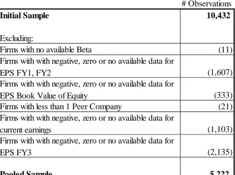
The initial sample comprised 10432 observations. This figure was then reduced to 5,222 due to no available relevant data for some observations (See Table 1)

# Observations

Initial Sample 10,432

Excluding:

Firms with no available Beta (11) Firms with with negative, zero or no available data for

EPS FY1, FY2 (1,607)

Firms with with negative, zero or no available data for

EPS Book Value of Equity (333) Firms with less than 1 Peer Company (21) Firms with with negative, zero or no available data for

current earnings (1,103) Firms with with negative, zero or no available data for

EPS FY3 (2,135)

Pooled Sample 5,222

(24)

24 (22)

(23) 3.2.2. - Division by Industry

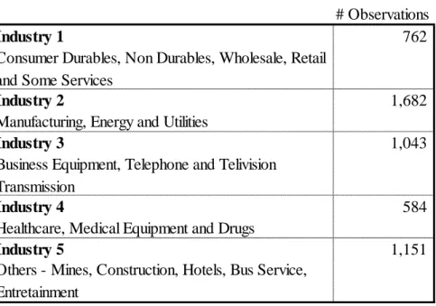
The pooled sample was divided in 5 independent industries in accordance to Fama French Framework (2013). Companies were allocated to industries by SIC codes as the framework defines (see Table 2).

The intention is to analyze R&D intensity within each industry. Empirical results tend to be more significant if companies which are being compared operate in similar industries, e.g. comparing a high tech pharmaceutical with an apparel producer may not be produce informative outputs for this study. This allows for an intra-industry analysis. Industry two and four are the ones expected to be more R&D intensive due to the nature of its activity (OECD, 2011), and thus, it is expected to see more relevant effect within this groups whereas the others are expected to produce lower

3.2.3. - Division within Industries considering R&D intensity

This study reproduces Ciftci, Lev and Radhakrishnan’s methodology (2009) to allocate companies to High/Low intensive R&D groups, as equations.

# Observations

Industry 1 762

Consumer Durables, Non Durables, Wholesale, Retail and Some Services

Industry 2 1,682

Manufacturing, Energy and Utilities

Business Equipment, Telephone and Telivision Transmission

Industry 4 584

Healthcare, Medical Equipment and Drugs

Others - Mines, Construction, Hotels, Bus Service, Entretainment

(25)

25 i’ to each group of 3-Digit SIC Codes

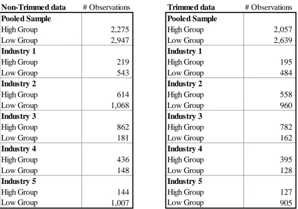
R&D intensity (22) of each firm is defined by the authors, and corroborated by OECD (2011), as the ratio of R&D expenditures to sales. Knowing that a company’ investment in R&D can deviate considerably from the mean of its competitors of the same industry in a certain year, a benchmark ratio (23) is considered for each 3-Digit Sic Code to avoid results to biased by this extraordinary events, e.g. a pharmaceutical company not investing in R&D in a certain year. Moreover, by using weighted average figures, the risk of being biased by companies’ size is avoided. A company is considered to be high (low) R&D intensive if the difference between its correspondent benchmark ratio and the weighted average R&D intensity of all industry is positive (negative). The allocation of observations is shown in table 3. Panel B is trimmed for outliers from all base variables of the four valuation models considered (see section 3.3.1.1), by excluding 1% on both tails, whereas Panel A is not. Hereafter, only trimmed data will be considered for statistical analysis in order to obtain robust and representative results. Note that ‘High Group’ (‘Low Group´) stands for high (low) R&D intensive groups.

Panel A Panel B

Non-Trimmed data # Observations Trimmed data # Observations

Pooled Sample Pooled Sample

High Group 2,275 High Group 2,057

Low Group 2,947 Low Group 2,639

Industry 1 Industry 1

High Group 219 High Group 195

Low Group 543 Low Group 484

Low Group 1,068 Low Group 960

Low Group 1,007 Low Group 905

Table 3 – Sample’s division by Industry and R&D intensity (trimmed and non-trimmed data)

‘High Group’ (‘Low Group’) stands for High (Low) R&D intensity. Industry Groups were defined by Fama French Framework. Note that Panel B represents trimmed data, by removing 1% on both tails for each variable (see Table 4).

(26)

26

3.2.4. Theoretical Models

Large Sample Analysis covers four valuation methods, identically distributed between Flow-Based and Stock-Based models. The two multiples models considered were 1-Year Forward PER and Price-to-Book whereas the two multi-period models are RIVM and OJM.. 1-Year Forward PER (hereafter mentioned as only ‘PER’), was chosen due to superiority of forward earnings as relevant driver (Liu et al, 2002). Price to book multiple (hereafter P/B) was chosen with the intention of having a book value multiple to compare with one based on earnings. RIVM was chosen as due to its superiority comparing to DCFM and DDM (Penman and Sougiannis, 1998; and Francis et al ,2000). Finally, OJM was chosen as it overcomes RIVM by substituting its anchor by discounted subsequent period capitalized earnings, instead of using book value of equity (Ohlson, 2005). Note that this study considers a simplified version of OJM where terminal value ceases to exist under a competitive environment

3.2.4.1. Peer Group Choice

Peers for each company are composed by entities with the same 3-Digit SIC Code. This option conflicts with Penman’s (2003) position as it is dangerous due to intra industries differences. Being aware of SIC Codes’ drawbacks for this purpose, this analysis considers the most effective SIC Code to select comparable companies, i.e. 3-Digit SIC Code (Alford, 1992).

3.2.4.1. Peer Group Choice

This study computes benchmark multiples for Stock-Based Valuation models using the harmonic mean as it produces the least biased results (Baker and Ruback, 1999).

3.2.4.3. Explicit Period

Main literature mentions that considering two years for explicit period produces significant enough results for RIVM and OJM. An alternative explanation would be to consider three years as explicit period as it helps to overcome GAAP’s reporting policies for R&D (Sougiannis and Yaekura, 2000).

(27)

27 (24) 3.2.4.4. Cost of Equity

The cost of equity computation follows the Capital Assets Pricing Model equation (see equation 24).

Where ‘ke’ stands for cost of equity of firm ‘i’ considering a risk free rate (rf) and market risk premium for year ‘j’ and company’s beta ( )

U.S. 10-Years Treasury was assumed to be the risk free rate (rf) for each year. The market return (rm) was computed by assuming the average annual compounding return of the S&P-500 from the last 20 years. The length of the period was chose in order to be long enough to avoid being biased by positive and negative peaks (e.g. Dot.com Bubble) and short enough to keep it realistic and actual. The market risk premium consists on the difference between market return and risk free rate. Finally, beta for each company is a levered figured withdrawn from CRSP database.

The cost of capital for each firm is them computed by summing the risk free rate to the product of beta and market risk premium. Note that robustness tests will be done further to measure sensitivity of market return to compute cost of equity.

3.2.4.5. Long Term Growth Rate

Long term rate (g) was assumed to be 2%. This figure only affects RIVM as OJM’s terminal period ceases to exist under a competitive environment. An alternative computation method would be multiplying firms’ beta and the growth forecast of U.S. GDP. Nasdaq Stock Exchange defines Beta as the metric that determines how firms’ returns move in comparison to market return. Despite being a strong assumption, using Beta for this purpose avoids the assumption of every company growing at the same rate, allowing similar companies to grow at similar paces. Note that a robustness analysis will be done further to measure sensitivity of long term growth rate.

(28)

28

3.2.4.6. Dividends Payout Rate

Dividend Payout Rate is defined by the ratio of dividends paid to earnings. This ratio is considered to remain constant for perpetuity in this analysis.

3.3. Empirical Finding

This section aims to analyze descriptive statistics and run a battery of tests to either corroborate or not hypothesis presented in section 3.1.

3.3.1. Descriptive statistics

A summary of descriptive statistics will be presented for relevant variables used in the large sample analysis. First, statistical properties for valuation models’ input variables (forecasted earnings, book value of share and market value of share) are going to be presented. Besides all relevant information regarding differences between groups and industries that can be taken from here, these statistical properties were used to trim data for outliers, by removing 1% on both tails on each variable. Second, descriptive statistics for valuation models’ output variables (prediction errors for four valuation models) will be summarized and commented, serving as background for all large sample analysis further statistical tests.

3.3.1.1. Valuation Models’ Input Descriptive Statistics

Table 4 summarizes main statistical properties of analyst’s forecasted earnings (‘EPS FY1’ and ‘FY2’) as well as book and market value of companies’ shares (‘Price’ and ‘BV p/share’). Results were trimmed for outliers by removing 1% on both tails on each variable as mentioned on section 3.2.3. Each panel corresponds to a single Fama French industry. There are significant differences between the five industries. Concerning the intra-industry groups (low and high R&D), these differences are not as significant, although industry 4 present the highest differences, followed by industry 2. This is not surprising since, according to the OECD (2011), these are the most R&D intensive industries. Thus, not engaging in this type of investment has natural consequences in terms of competitive advantage for firms operating in these industries, reducing profitability levels and

(29)

29 share price. On the other hand, R&D intensity seems to have a minor influence on the forecasted EPS and share price industries for industries 1, 3 and 5, where the differences between groups are lower. It is also interesting to note that mean and median figures of firms’ market value are larger for industries 2 and 4 than for the remaining others. Despite being a 'per share measure', this suggests that firms operating in more R&D intensive industries tend to be more valued by the market. A pattern that is shared by almost all industries is that of the mean and median of the 'book value' of the share to be greater for lower R&D intensive firms. This is consistent with the position of 'Sougiannis and Yaekura (2000)', which says that policies accounting GAAP are complex and confusing when it comes to R&D expenditures, recognizing it often as expenses instead of investments, which consequently decreases book values.

Table 4 – Input Descriptive of Valuation Models

‘EPS FY1’, ‘EPS FY2’, ‘Price p/s’ and ‘BV p/s’ stands for forward earnings per share year 1 and 2, price per share and book value per share, respectively. ‘MN’, ‘SD’, ‘MD’, ‘Q1’, ‘Q3, ‘Max’, ‘Min’ stands for Mean, Standard Deviation, Median, Quartile 1, Quartile 3, Maximum and Minimum, respectively. Note that data are timed for outliers by removing 1% on both tails for each variable

(30)

30

3.3.1.2. Valuation Models’ Output Descriptive Statistics

Table 5 summarizes statistical properties of prediction errors of the four valuation methods used in this analysis. Each panel corresponds to a Fama French industry. Signed Prediction errors measure bias whereas absolute prediction errors measure accuracy of valuation models. The closest these figures are to zero, less biased and more accurate are models. If signed prediction errors are negative (positive) means model to undervalue (overvalue) firm in comparison with market share price.

In this study median will be used either to compare industries or intra-industry’s groups. The choice for median over mean is related to the lower sensitivity of the first to extreme values (outliers), that were removed only for valuation methods’ inputs as mentioned on section 3.3.1.1. This way, median appears as a more stable indicator (Damodaran, 2002) for comparison between industries and intra-industry’s groups. Over all industries and groups it is possible to identify a general trend of lowest variation in signed prediction errors of PER valuation method, followed by P/B, RIVM and OJM. There is a trend for stock-based valuation methods to be less biased than flow-based valuation methods. Regarding absolute prediction error, the analysis also suggest a general trend of lowest variation of PER valuation, followed by OJM and P/B (both models share the second place in this matter) and RIVM.

Whilst PER seems to be the less biased and more accurate model, OJM seems to be more accurate than unbiased, which is surprising. In general, stock-based valuation methods seems to be less unbiased and more accurate than flow-based valuation methods which is also surprising and contradicts Palepu et al (2000), Copeland et al (2000) and Penman (2001) preference for multi-period models. Thus, this might suggest the rejection of the third hypothesis, that will be tested further. There are some explanations for this finding, e.g. flow based models might be specified over unrealistic assumptions or it might be related with the fact that only two periods were considered for the explicit period.

There are also significant differences in signed and absolute prediction errors between industries and between groups, suggesting that to be less accurate and more biased for high groups and high R&D intensive industries. It is also important to mention that the fact that models used tend to undervalue firms for all groups, as more than three quarters of signed prediction errors values are negative.

(31)

(32)

(33)

33

3.3.3. Hypotheses Tests for Prediction errors

This section follows the analysis of Penman and Sougiannis (1998) and Francis et al (2000) and summarizes main finding of a battery of tests regarding signed and absolute prediction errors. Median is the indicator chosen to run the tests as it is more stable than the Mean (Damodaran, 2002). This way, all hypotheses tests will be non-parametric.

First, tests will be applied both for the median of signed and absolute prediction errors for all models in all groups to see its significance. Second, hypotheses test will be conducted comparing the median of absolute errors of single models between high and low R&D intensive groups in each industry. Finally, hypotheses tests will be made to compare median of absolute prediction errors of all valuation models for all groups.

Table 6 shows p-values for significance level tests for median of both signed and absolute prediction error of valuation models. Null hypothesis of this test is Median to be equal to zero.

At a 5% significance level, the null hypothesis is rejected for absolute prediction errors of all models, in any industry or group, meaning that there is no support for the hypothesis that accuracy of models is perfect. On the other hand, for the same level of significance, the null hypothesis is not rejected for almost all signed prediction errors of PER valuation method, as well as some values of P/B, suggesting a higher strength of these models in terms of bias.

(34)

34 Table 7 shows p-values for Wilcoxon Rank Sum tests (two independent samples test) comparing median of bias and accuracy of models between high and low groups, within each industry. The null hypothesis is the median of prediction errors of singles valuation methods to be equal both for high and low group, within each industry.

There are significant differences in terms of models’ bias and accuracy between high and low groups. These differences are higher for industry for theoretical lower intensive R&D (OECD, 2011), i.e. industry one, two and three. At a 5% significance level, it is possible to observe that null hypothesis is only rejected for all valuation Models when absolute prediction errors are tested for industry 2 and 4. It suggests that not only differences, in terms of models’ bias, between high and low groups are lower in theoretical higher R&D intensive industries but also that these differences are not statistical significant (at a 5% significance level) when it comes to accuracy of Models. There are then support for hypothesis 1 only for industries 2 and 4, since R&D intensity affects bias and accuracy of valuation models for high R&D intensive industries.

Table 6 – Significance Level Tests for Median of Prediction Errors

Table 6 shows p-values for significance level tests for median of both signed and absolute prediction error of valuation models. Null hypothesis of this test is Median to be equal to zero. Signed (Absolute) Prediction Errors measure bias (accuracy) of valuation models. Signed Prediction Errors for each observed firm is measured by:

whereas Absolute Prediction errors are the absolute value of this figure.

‘PER, ‘P/B, ‘RIVM and ‘OJM’ stands for Price Earnings Ratio, Price to Book ratio, Residual Income Valuation Model and Ohlson Juettner-Nauroth Model, respectively. ‘Note that data are timed for outliers by removing 1% on both tails for each variable

(35)

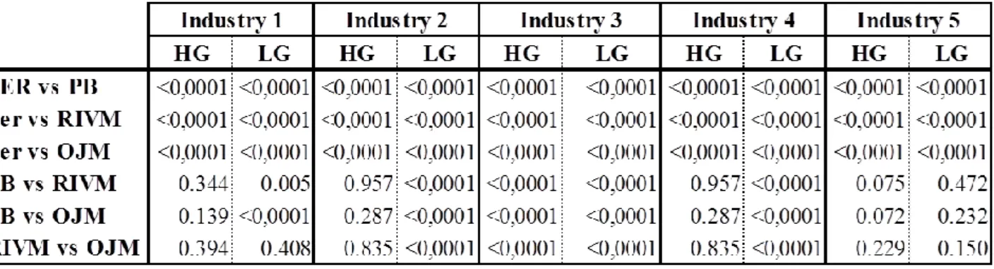
35 Table 8 shows p-values Wilcoxon Signed Rank tests (related samples test) comparing median of bias and accuracy between models, within each industry and intra-industry groups. Null hypothesis is that Median of prediction errors of two different valuation methods to be equal.

The null hypothesis is rejected more often when two models are compared for high R&D intensive groups. Thus, differences between models in terms of bias and accuracy appear to exist and to be higher for high groups, suggesting R&D intensity to influence choice for valuation methods (support for hypothesis 1).

Table 7 shows p-values for Wilcoxon Rank Sum tests (two independent samples test) comparing median of bias and accuracy of models between high and low groups, within each industry. The null hypothesis is the median of prediction errors of singles valuation methods to be equal both for high and low group, within each industry. Signed (Absolute) Prediction Errors measure bias (accuracy) of valuation models. Signed Prediction Errors for each observed firm is measured by:

whereas Absolute Prediction errors are the absolute value

of this figure. ‘PER, ‘P/B, ‘RIVM and ‘OJM’ stands for Price Earnings Ratio, Price to Book ratio, Residual Income Valuation Model and Ohlson Juettner-Nauroth Model, respectively.

Table 7 – Wilcoxon Rank Sum tests, comparing prediction errors of valuation models between high and low groups.

(36)

36

3.3.4. Linear Regression and Robustness Test

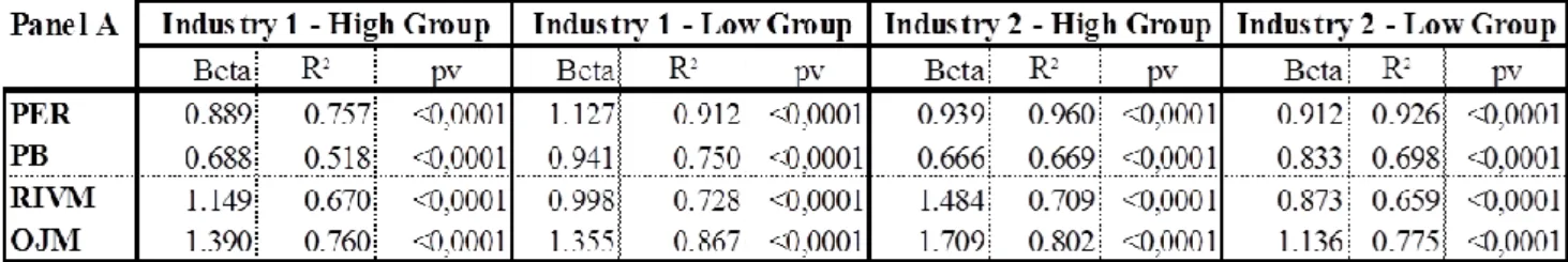
Table 9 shows the output for linear regressions performed in this analysis. The independent variables are the valuations computed by each of the four valuation methods for each firm whereas the dependent variable is the market share price for each company. Only one independent variable was regressed against share price and interception was not considered. Beta represents slope of independent variable, R-squared represents the percentage of dependent variable values which are explained by independent variable (explanatory power) and p-value (pv) is a measure of significance of slopes.

All slopes are statistically significant, meaning that independent variables are relevant to explain share price. PER valuation method seems to have the highest explanatory power, followed by OJM, RIVM and P/B, suggesting a higher performance of PER over flow-based valuation methods adopted.

R&D intensity appears to influence explanatory power of Models as high groups present higher Table 8 – Comparison of prediction errors between valuation models within groups.

Table 8 shows p-values Wilcoxon Signed Rank tests (related samples test) comparing median of bias and accuracy between models, within each industry and intra-industry groups. Null hypothesis is that Median of prediction errors of two different valuation methods to be equal.

Signed (Absolute) Prediction Errors measure bias (accuracy) of valuation models. Signed Prediction Errors for each observed firm is measured by:

whereas Absolute Prediction errors are

the absolute value of this figure. ‘PER, ‘P/B, ‘RIVM and ‘OJM’ stands for Price Earnings Ratio, Price to Book ratio, Residual Income Valuation Model and Ohlson Juettner-Nauroth Model, respectively.

(37)

37 values of r-squared than low groups, giving support to hypothesis 2. At the same time, industry in which a company operates also seems to influence explanatory power as theoretical lower R&D intensive industries have lower values of r-squared, supporting hypothesis 1. Finally, PER seems to be the models with higher explanatory power, contradicting hypothesis 3.

Table 9 – Linear Regressions’ output.

Table 9 shows the output for linear regressions performed in this analysis. The independent variables are the valuations computed by each of the four valuation methods for each firm whereas the dependent variable is the market share price for each company. Only one independent variable was regressed against share price and interception was not considered. Beta represents slope of independent variable, R-squared represents the percentage of dependent variable values which are explained by independent variable (explanatory power) and p-value (pv) is a measure of significance of slopes. ‘PER, ‘P/B, ‘RIVM and ‘OJM’ stands for Price Earnings Ratio, Price to Book ratio, Residual Income Valuation Model and Ohlson Juettner-Nauroth Model, respectively.

(38)

38 The explanatory power of flow-based valuation models is highly sensitive to assumptions methods adopts. This way, table 10 shows explanatory power of models when two of the most sensitive assumptions, long term growth rate (g) and market return (Mr), varies. Growth rate affects only RIVM as this study considers a simplified version of OJM, where terminal value ceases to exist under a competitive environment.

Be presenting higher variation in r-squared, long term growth rate appears to be a more sensitive assumption than market return. This analysis also suggests assumptions assumed for models to be too much conservative. Considering a higher long term growth rate and a lower market return would result in higher explanatory power for flow-based valuation models. Nevertheless, if this reviews explanatory power is compared with PER’s (see table 9), it is possible to conclude that the stock-based valuation method still presents higher explanatory power over the two flow-based valuation models.

Robustness testing concludes assumptions adopted to be conservative, in particular long term growth rate. Nevertheless, it does not change conclusions for hypothesis 1,2 and 3 (support or not).

(39)

(40)

40

3.3.5. Association Test

This section aims to measure the association between company’s size (market capitalization) and R&D intensity. This analysis is performed by making a chi-square (by comparing first and fourth quartile of variables through a contingency table) test and only includes high R&D intensity groups within each industry. If lower groups were included the results would be biased by R&D intensity of these firms, which is near 0% for every firm. Moreover, if low intensive firms were included statistical software (e.g. SAS or SPSS) would report an error as the first quartile of R&D intensity would be composed by a constant (0%). This way, the test is more robust and significant as it compares similar companies in this matter.

Table 11 shows p-value of Chi-square test for every high R&D intensive groups within each industry. The null hypothesis is that no association exists between firm size (market capitalization) and R&D intensity.

At a 5% significance level, null hypothesis is not rejected for theoretical higher R&D intensive industries (OECD, 2011), i.e. two and four and rejected for all others. The result suggests R&D intensity to be associated with firm size only in low R&D intensive industries and it may be explained by the nature of each industry’s operation. Whilst in theoretical higher intensive industries R&D expenditures is part of the core business and companies are forced to engage in it in order to remain competitive, in the remaining industries this investments are not considered to be core and are only engaged by bigger firms.

High Groups p-value

Industry 1 0.310 Industry 2 0.024 Industry 3 0.071 Industry 4 0.025 Industry 5 0.916

Table 11 – Association Test.

Table 11 shows p-value of Chi-square test for every high R&D intensive groups within each industry. The null hypothesis is that no association exists between firm size (market capitalization) and R&D intensity.

(41)

41 3.4. Concluding Remarks

The analysis of descriptive statistics and the batteries of tests engaged in the large sample analysis allowed to decide either if there is support for the four hypotheses or not. The results were that there are support hypotheses 1 and 2, no support hypothesis 3 and partial support for hypothesis 4.

3.4.1. Support for Hypothesis 1

By running a battery of Wilcoxon Rank Sum tests (two independent samples) for the difference of signed and absolute prediction errors of models between high and low groups it is possible to conclude that R&D intensity as well as industry groups affect both bias and accuracy of flow based valuation models and does not affect bias of stock based valuation models. It is possible to see that differences between high and low groups are more significant for industries 2 and 4, which are the theoretical more R&D intensive industries. Results are supported by linear regression analysis that despite testing only explanatory power, it is possible to observe significant differences between industries. Results are consistent with Amir and Lev’s (1996) argument that non-financial information is needed when valuing R&D intensive firms.

3.4.2. Support for Hypothesis 2

The linear regression r-squared results suggest that models have lower explanatory power when valuing high R&D intensive firms, which is consistent with Amir and Lev (1996) results. Note that robustness test results does not change support for this hypothesis.

3.4.3. No Support for Hypothesis 3

Linear Regression suggests PER method to be the one with greatest explanatory power, followed by OJM, RIVM and P/B. Moreover, a battery of Wilcoxon Signed Rank tests (paired samples) for the difference of absolute prediction errors of two different valuation models within each group suggest accuracy to differ from model to model. This is not consistent with the theoretical equality of models.

(42)

42

3.5.4. Partial Support for Hypothesis 4

The results of Chi-Square tests (using a contingency table) suggest firms’ size to be associated with R&D intensity only in industry 2 and 4. Note that the tests were only applied for high R&D intensive groups in order to ensure the robustness and statistical significance.