International equity risk premium predictability in the frequency domain

International equity risk

premium predictability in the

frequency domain

Final Assignment in the modality of Dissertation presented to Universidade Católica Portuguesa for obtaining the degree of Master in Finance

by

Fernando Miguel Xavier Mariz

under the supervision of

(PhD) Gonçalo Faria and (PhD) Fabio Verona

Católica Porto Business School March of 2018

Acknowledgments

I would like to thank everyone that supported me during this assignment. To my parents, Fernando and Isabel, without whom I wouldn’t have made it so far, I owe it all to them.

To my supervisors, Professor Gonçalo Faria and Professor Fábio Verona, for the knowledge transmitted, guidance and permanent availability along this challenging and rewarding journey.

To Benedita, for the help provided in this dissertation and for the constant presence and interest.

To all my closest family, especially my sister and friends for the motivation and support provided both directly and indirectly.

Resumo

Nesta dissertação, estendemos o método SOPWAV de Faria e Verona (2018), que foi desenvolvido para prever o retorno das ações no mercado dos Estados Unidos da América, para mercados internacionais. O SOPWAV é baseado no método sum of the parts (SOP) proposto por Ferreira e Santa Clara (2011), que decompõe o retorno das ações em três partes diferentes, com o objetivo de, num primeiro momento, estimar cada uma destas separadamente e, num segundo momento, somá-las para obter a previsão do retorno das ações. O SOPWAV usa as frequências das três partes referidas, em vez das séries temporais originais (utilizadas no SOP), para as estimar, através de métodos de decomposição de onduletas. O método SOPWAV permite isolar as frequências das partes dos retornos das ações que contêm maior poder preditivo. Através dos resultados obtidos, percebemos que este método melhora significativamente a previsão dos retornos das ações na amostra dos países analisados, nomeadamente, Japão, Reino Unido, França, Alemanha, Canada, Suíça, Austrália e África do Sul. Para além de melhorar a previsão dos retornos, o método SOPWAV, de um modo geral, permite também maiores ganhos de utilidade para um investidor, quando comparados com a média histórica e o SOP; ganhos de utilidade, comprovados em estratégias de trading, que foram simuladas no decorrer desta investigação.

Palavras-chave: Previsão do Retorno das Ações, Mercados Internacionais, SOPWAV, Domínio da Frequência

Abstract

In this dissertation, we extend the Faria and Verona (2018) SOPWAV method for forecasting US stock market returns to international stock markets. The SOPWAV has its roots in the sum of the parts (SOP) method proposed by Ferreira and Santa Clara (2011), that decomposes stock returns in three different parts, and forecasts them separately to obtain the estimated stock returns. The SOPWAV method uses the frequencies of those components, instead of their original time-series which are obtained through a wavelet decomposition. The SOPWAV method allows to isolate the frequencies of the stock return parts that have the highest predictive power. We found evidence that this method significantly improves predictability across the sample of countries tested (Japan, United Kingdom, France, Germany, Canada, Switzerland, Australia and South Africa) and delivered higher utility gains than the SOP method and the traditional benchmark (historical mean) in trading strategies simulated throughout this investigation.

Keywords: Stock return predictability, International stock markets, SOPWAV, frequency domain

Contents

Acknowledgments ... iii

Resumo ... v

Abstract ... vii

List of Figures ... xi

List of Tables ... xiii

Introduction ... 15

Literature Review ... 17

1.1. Forecasting stock returns ... 17

1.1.1. International stock returns ... 21

1.2. Frequency domain in economic and financial topics ... 24

Data and Methodology ... 29

2.1. Data description ... 29

2.2. Methodology ... 34

2.2.1.The SOP decomposition ... 34

2.2.2. Time-frequency decomposition of economic time series ... 36

2.2.3. Forecasting with the SOPWAV method ... 40

2.2.4. Out-of-sample forecasts ... 43 2.2.5. Forecast evaluation ... 44 Empirical Results ... 47 3.1. Statistical Performance ... 47 3.1.1.Out-of-sample period: 02/2000 to 10/2017 ... 48 3.1.2.Out-of-sample period: 01/1990 to 10/2017 ... 56 3.2. Robustness Tests ... 57 3.2.1.Alternative Multiple ... 57

3.2.2.Forecasting the U.S. stock returns ... 59

3.3. Trading Strategy ... 60

Conclusion ... 65

Bibliografy ... 67

List of Figures

List of Tables

Table 1. Out-of-sample R-squares (in percentages) for Japan ... 48

Table 2. Out-of-sample R-squares (in percentages) for the United Kingdom .. 49

Table 3. Out-of-sample R-squares (in percentages) for France ... 50

Table 4. Out-of-sample R-squares (in percentages) for Germany ... 51

Table 5. Out-of-sample R-squares (in percentages) for Canada ... 52

Table 6. Out-of-sample R-squares (in percentages) for Switzerland ... 53

Table 7. Out-of-sample R-squares (in percentages) for Australia ... 54

Table 8. Out-of-sample R-squares (in percentages) for South Africa ... 55

Table 9. Out-of-sample R-squares (in percentage) for the whole sample of countries in the forecast period of 01/1990 to 10/2017 ... 56

Table 10. Out-of-sample R-squares (in percentage) for the whole sample of countries in the forecast period of 01/2000 to 10/2017 using the price-earnings growth rate. ... 58

Table 11. United States performance ... 60

Table 12. Annual percentage CER gains ... 63

Introduction

The highly debated topic of forecasting stock returns has been in the mind of researchers and practitioners of finance for quite some time.

For practitioners it is of utmost importance to understand the functioning of financial markets and especially real-time forecasted stock returns, as this provides a means to enhance asset allocation and ultimately the investor performance. From an academic standpoint, forecasting stock returns is important for many reasons, including the ability of using more realistic asset pricing models and improving the understanding of different factors that depend on stock returns.

But the task of forecasting stock returns is a very challenging one, translated in the fact that most of the existing forecasting models only explain a small part of the stock returns. Also, in line with the arbitrage pricing theory and the efficient market hypothesis, one of the problems in constructing models that can effectively forecast a small part of the stock returns is the fact that the forecast will be arbitraged away. More specifically, as investors start trading with the new information available to the public (in this case the hypothetical new model) the markets will adjust to incorporate that same information, which will lead to the disappearance of the model ability to predict stock returns (e.g., Timmermann and Granger (2004) and Timmermann (2008)).

Our work builds on the Faria and Verona (2018) SOPWAV method for forecasting stock returns, which is based on the Ferreira and Santa-Clara (2011) sum of the parts (SOP) method. In a nutshell, the SOP method consists in

decomposing the stock market return into three parts, forecasted separately, which leads to an improved forecast accuracy by exploiting the different time series persistence of the three parts.

The innovation of the SOPWAV method is that it forecasts the stock return parts by selectively summing some of the frequency-decomposed parts of the stock market returns, instead of summing the original parts (as in the SOP method).

It is shown that, for the US stock market, the SOPWAV method delivers statistically and economically significant gains for investors, outperforming both the historical mean benchmark and the SOP method. The objective of this dissertation is to extend the application of the SOPWAV methods to international stock markets (i.e. non U.S. equity markets) and to find if the out-of-sample predictability of the equity risk premium in international markets can also be improved by considering frequency-decomposed predictors. The countries selected for this analysis were Japan, United Kingdom, France, Germany, Canada, Switzerland, Australia and South Africa.

We obtained positive significant at the 1% level out-of-sample R-squares for every country under analysis as well as a demonstration of the utility gains for an investor that uses a trading strategy for those countries based on the SOPWAV.

The rest of the dissertation is structured as follows. In Chapter 1 we review related literature in forecasting returns (for both the United States and international markets), as well as using frequency decomposition methods in financial topics. In Chapter 2 we explain the data and the methodology used and in Chapter 3 we provide the empirical results, as well as the robustness tests and trading strategy

Chapter 1

Literature Review

The SOPWAV method relates with two branches of literature. The first one refers to out-of-sample (OOS) stock return predictability. The second one has to do with the application of wavelets decomposition methods and the use of frequency domain in financial topics. In the following two subsections we briefly review these two branches of literature.

1.1. Forecasting Stock Returns

Attempts to predict stock returns have a long tradition in finance, since a reliable forecast provides a crucial part in the computation of the cost of capital and the investment process in general. As pointed by Goyal and Welch (2008) “The literature is difficult to absorb. Different articles use different techniques, variables, and time periods. Results from articles that were written years ago may change when more recent data is used and some articles contradict the findings of others.”

It is possible to assume a general time-series of stock returns predictability, as pointed by Henkel et al. (2011), who presents the beginning of the time series as being the Fama (1965, 1970) random walk theory, in which stock returns were assumed to follow a random walk. After, the use of the short rate followed as a predictor of stock returns (Fama and Schwert (1977), Fama (1981), Geske and Roll

(1983)), then came the dividend yield predicts (Rozeff (1984), Shiller (1981)) followed by the term premium predicts (Campbell (1987), Fama (1984), Keim and Stambaugh (1986), Harvey (1988) and the default premium predicts (Chen et al. (1986), Keim and Stambaugh (1986)) which lead to some debate about predictability (Goetzmann and Jorion (1993), Hodrick (1992), Kim and Nelson (1993), Richardson and Stock (1989)) and eventually there was some illusion and disbelief in predictability present in the works of Bossaerts and Hillion (1999), Brennan and Xia (2005), Ang and Bekaert (2007), Cochrane (2008), Goyal and Welch (2003, 2008) and Valkanov (2003) who address some issues related to forecastability, namely lack of robustness out-of-sample.

To predict stock returns, usually a typical specification regresses an independent lagged predictor on the stock market rate of return:

𝑆𝑡𝑜𝑐𝑘 𝑅𝑒𝑡𝑢𝑟𝑛𝑠𝑡 = 𝛽0+ 𝛽1𝑥𝑡−1+ 𝜀𝑡 (1)

Where 𝛽1 is a measure of how significant is the 𝑥 variable in predicting stock returns, that has been constantly explored through the years.

In the 1960s a series of studies examined the forecasting power of various technical indicators, including popular filter rules, moving averages, and momentum oscillator (Alexander (1961, 1964), Cootner (1962), Fama and Blume (1966) and Jensen and Benington (1970)).

Beginning in the late 1970s a search for predictors began, as a vast literature provided evidence that multiple economic variables predicted monthly, quarterly, and/or annual U.S. aggregate stock returns in predictive regressions. The most popular predictors used in these investigations were the dividend-price ratio (Rozeff (1984); Campbell and Shiller (1988a, 1998); Hodrick (1992); Fama and French (1988, 1989); Cochrane (2008); Lettau and Van Nieuwerburgh (2008); Pastor and Stambaugh (2009)), the earnings price-ratio (Campbell and Shiller

(1988b), (1998)), book-to-market ratio (Kothari and Shanken (1997); Pontiff and Schall (1998), nominal interest rates (Fama and Schwert (1977); Breen et al. (1989); Ang and Bekaert (2007)), interest rate spreads (Campbell, 1987; Fama and French, 1989), inflation (Nelson (1976); Campbell and Vuolteenaho (2004)), dividend-payout ratio (Lamont (1998)), corporate issuing activity (Baker and Wurgler (2000); Boudoukh et al. (2007)), consumption-wealth ratio (Lettau and Ludvigson (2001), stock market volatility (Guo (2006)), labor income (Santos and Veronesi (2006)), aggregate output (Rangvid (2006)), output gap (Cooper and Priestly (2009)), expected business conditions (Campbell and Diebold (2009)), oil prices (Driesprong et al. (2008)), Jagged industry portfolio returns (Hong et al. (2007)), and accruals (Hirshleifer et al. (2009).1

Furthermore, Pesaran and Timmermann (1995) address the importance of model uncertainty and parameter instability when forecasting stock. This makes the selection of a consistently robust predictive model through time a very challenging task.

Moreover, although business cycles are not considered in this dissertation they are naturally linked with stock returns forecast. This results from the fact that asset returns are functions of an extensive set of macro and microeconomic variables linked with the business cycles fluctuations

Related with this, Henkel et al. (2011) investigated the stock return predictability in G7 countries and found a strong and robust link between the extent of aggregate return predictability and the business cycle in all of the G7 countries excepts Germany and also that “the short-horizon performance of aggregate return predictors such as the dividend yield and the short rate appears non-existent during business cycle expansions but sizable during contractions”.

1 _{The authors considered are just a representative sample, as there are many more investigations that uses}

These results are in line with the ones presented in Rapach, Strauss and Zhou (2010), which found that stock return predictability is countercyclical.

Still, most readers are left with the impression that prediction works, or as Lettau and Ludvigson (2001) state: “It is now widely accepted that excess returns are predictable by variables such as dividend-price ratios, earnings-price ratios, dividend-earnings ratios, and an assortment of other financial indicators.”

Noting that predictive models require out-of-sample validation, Goyal and Welch (2008) demonstrated how most of the models up until that time performed poorly out-of-sample. As forecast models require out-of-sample predictability, to overcome this issue, Faria and Verona (2018) point out that “researchers have since then turned their attention to improving the out-of-sample forecastability of stock returns, exploring two different avenues”. The first avenue of research to overcome poor out-of-sample results focuses on developing and testing new predictors, while the second on improving existing forecast methods.

Works that relate with testing new predictors include Bollerslev et al (2009) that test the variance risk premium, Rapach et al explores the role of lagged U.S. market returns for the out-of-sample predictability for other countries, Li et al (2013) demonstrates that the implied cost of capital predicts stock returns predicts stock returns, Jordan et al (2014) uses two new technical variables (the ratio of rising stocks to fallers and the change in trading volume) and Neely et al. (2014) consider the relevance of several technical indicators to serve as complementary predictors for the common ones within the literature.

Some researches made that relate to improving existing models to overcome poor out-of-sample performance are for example Ferreira and Santa Clara (2011), who introduced the SOP method, Dangl and Halling (2012) who evaluated predictive regressions that considered the time-variation of coefficients, Pettenuzzo, Timmermann and Valkanov (2014) that proposed imposing constraints on time series forecasts of the equity premium, Lima and Meng (2017)

proposes a quantile combination approach and Faria and Verona (2018) who introduced the SOPWAV method.

1.1.1. International Stock Returns

Most of the literature regarding this subject is focused on the U.S. stock market returns, although there are exceptions.

Harvey (1991) examines the discrepancy in average stock returns across industrialized countries by measuring the conditional risk of 17 countries and concludes that “the results show that countries' risk exposures help explain differences in performance.” Meanwhile, Bekaert and Hodrick (1992) characterize the predictable components of returns on major international exchange markets using lagged excess returns, dividend yields, and forward premiums as instruments. Campbell and Hamao (1992) study the integration of long-term capital markets in the U.S and Japan, by using the monthly excess return predictability of those countries, and they find that U.S. variables (such as the lag-returns) help to forecast excess Japanese stock returns. This led to the consideration of U.S. lagged returns as being a good predictor of non-U.S. financial markets, as studied by Rapach, Strauss and Zhou (2013), who found that U.S. has a leading role, given that its lagged returns significantly predict returns in numerous non-U.S. industrialized countries, while lagged non-U.S. returns display limited predictive ability with respect to U.S. returns.

Ferson and Harvey (1993) investigated predictability in national equity market returns, and its relation to global economic risks in 18 equity markets and demonstrate how to consistently estimate the fraction of the predictive variation that is captured by an asset pricing model for the expected returns.

With the exception of Rapach et al (2013), the investigations provided above were among the first significant international stock return predictability studies conducted.

More recently, Schmeling (2009) examined whether consumer confidence affected expected stock returns in 18 industrialized countries and found that sentiment negatively forecasts aggregate stock market returns on average across countries and that when sentiment is high, future stock returns tend to be lower and vice versa. Engsted and Pedersen (2010) provide international evidence on stock returns and dividend growth predictability on long-term data from Denmark, Sweden and the United Kingdom and show that predictability patterns in three European stock markets are in many ways different from what characterize the US stock market. Hjalmarsson (2010) conducts tests in search of stock return predictability in the largest data set analysed so far, using four common forecasting variables (the dividend-price ratio, earnings-price ratio, short interest rate and the term spread), in a sample that comprises of 20000 monthly observations for 40 international markets. Across the sample, he concluded that traditional valuation measures such as the dividend-price and earnings-price ratios have very limited predictive ability in international data. However, he noted that using methods that do not account for the persistence and endogeneity of these variables would lead one to vastly misjudge their predictive powers and that interest rate variables are better predictors of stock returns, although their predictive power is mostly evident in developed markets. Narayan et al (2014) test for predictability of excess stock returns for 18 emerging markets and finds some evidence of in-sample predictability for 15 countries. And also shows that investors in most countries where short-selling is prohibited could make significant gains if limited borrowing and short-selling were allowed.

Henkel et al. (2011) carries out an investigation on the G7 countries to prove that “the short-horizon performance of aggregate return predictors such as the dividend yield and the short rate appears non-existent during business cycle expansions but sizable during contractions. This phenomenon appears related to

countercyclical risk premiums as well as the time-variation in the dynamics of predictors. Our empirical model outperforms the historical average out-of-sample in the US, but the results throughout the G7 are mixed.”

Thomadakis (2016) focuses on forecasting German stock returns and finds that the term spread has the in-sample ability to predict stock returns, delivering consistent out-of-sample forecast gains relative to the historical average, and also that combination forecasts do not appear to offer a significant evidence of consistently beating the historical average forecasts of the stock returns. This evidence of both in-sample and out-of-sample predictability of stock returns from the term spread is in line with some literature on the subject for the U.S. (e.g. Faria and Verona (2017)).

Jordan, Vivian and Wohar (2014) examines in-sample (INS) predictability but focuses on out-of-sample (OOS) forecasting of stock returns while using a big sample of 14 European countries with differing characteristics, that had none or very little prior OOS forecasting evidence. Jordan et al. (2014) also consider three types of predictor variables (fundamental ratios, macro variables, and technical variables) can forecast stock returns. Additionally, he examined if methods proposed to overcome poor return predictability can improve forecast accuracy or increase economic value. Lawrenz and Zorn (2017) conduct an analysis on 27 equity indices by taking the perspective of international asset allocation. The paper intends to test if predictive regressions conditional on time-series and cross-sectional information can improve forecasts of stock index returns by using different current price-to-fundamental ratios as predictors and by conditioning the sample on the indicator if time-series and cross-section deliver consistent or opposing signals.

Most of these studies estimate in-sample predictive regressions for non-U.S. country returns by using a variety of domestic and/or U.S. variables as predictors.

One of the main conclusions from these investigations is that stock returns offer the same degree of predictability in an international context as in the U.S.

However, not all studies hold up when assessing out-of-sample performance; of the ones previously cited, only Hjalmarrson (2010), Henkel et al. (2011), Rapach

et al. (2013), Thomadakis (2016), Jordan, et al. (2014), Narayan et al. (2014) and

Lawrenz and Zorn (2017) conduct out-of-sample tests with promising results in some of the countries analysed.

Given the literature on the subject, we can assume that in addition to the U.S. aggregate market, there is significant out-of-sample evidence of stock return predictability for other countries as well. Moreover, based on the out-of-sample predictability in international and cross-sectional returns, an investor can produce sizable utility gains from an asset allocation perspective.

We will analyse the out-of-sample forecasting performance of several international countries when using frequency domain based model (SOPWAV).

1.2. Frequency domain in economic and financial topics

The use of frequency domain, although highly popular in other topics, is still relatively unexplored in the financial/economical areas. A particular frequency domain technique is the wavelet transform, which has been particularly useful for analysing signals that can be considered as noisy, aperiodic or intermittent. This proves to be a valuable tool when addressing investigations in areas such as “geophysics, for the analysis of oceanic and atmospheric flow phenomena, seismic signals and climatic data; in medicine, for heart rate monitoring, breathing rate variability and blood flow and pressure; in engineering, for the assessment of machine process behaviour”, Rua (2011).

The attractiveness of using this method in the study of finance and economic topics comes from an idea presented in Adisson (2017) as the data sets (stock market indices, commodity prices, exchange rates, real estate prices, growth data,

mortgages, etc.) are typically highly non-stationary and demonstrate significant complexity and involve both random processes and intermittent processes. Therefore, as a way to overcome this “problem”, wavelet decomposition proves to be a very useful tool as Ranta (2010) states “Wavelet techniques possess an inherent ability to decompose this kind of time series into several sub-series which may be associated with a particular time scale. Processes at these different time-scales, which otherwise could not be distinguished, can be separated using wavelet methods and then subsequently analysed with ordinary time series methods”. This allows an investigator to unveil relationships between economic variables in the time-frequency space and to access simultaneously how variables are related at different frequencies and how that same relationship evolved through time. In this way, "Wavelets are treated as a ’lens’ that enables the researcher to explore relationships that previously were unobservable", according to Ramsey (2002), and it also allows us to “say that with wavelet methods we are able to see both the forest and the trees” as pointed out by Ranta (2010).

Gençay et al. (2001a) argue that wavelet methods provide insight into the dynamics of economic/financial time series beyond that of standard time series methodologies. Wavelets also work naturally in the area of non-stationary time series, unlike the Fourier methods, which are crippled by the necessity of stationarity.

The main difference between both analyses (wavelet and Fourier) is that the wavelet transform has the ability to separate the dynamics in a time series over a variety of different time horizons, thus maintaining both frequency domain and time domain information, while in the Fourier spectral analyses, time domain information is lost. Howell and Mahrt (1997) noted that using a wavelet based multi-resolution analysis (MRA) decomposition in place of the Fourier analysis

for examining a quasi-stationary turbulent time series has the advantage of matching the MRA average length to the width of a localized event.

There are several examples of wavelet methods which have a lot of potential in economics and finance. The maximal overlap discrete wavelet transform (MODWT) (Percival & Walden (2000)) is one of them, which is a modification of the ordinary discrete wavelet transform, and different from the continuous wavelet transform as Rua (2011) describes “In the continuous wavelet transform, the wavelets used are not orthogonal and the data obtained by this transform are highly correlated. In fact, in a non-orthogonal wavelet analysis an arbitrary number of scales can be used to provide a complete picture. In contrast, the discrete wavelet transform decomposes the signal into a mutually orthogonal set of wavelets.”

In the fields of economics and finance, wavelet based methods have been used for example to study the relationship between several macroeconomic variables, namely money supply and output in the first case and consumption and income in the second (Ramsey and Lampart (1998a,b). Kim and In (2003, 2005) investigate the relationship between financial variables and industrial production and between stock returns and inflation respectively. Tiwari et al. (2013) assess oil price dependence via wavelet analysis. Reboredo and Riveira-Castro (2014) analyse dependency between oil prices and stock returns. Fernandez (2005, 2006) studies the Capital Asset Pricing Model at different scales. Lo Cascio (2007) decomposes UK real gross domestic product via wavelet filter so as to investigate the long-run structure of the data apart from external shocks and He et al. (2012) use a multivariate wavelet method to investigate the dynamics of correlations for international markets. Additional research using wavelets includes the study of the relationship between oil and stock markets in the G7 countries by Khalfaoui, Boutahar and Boubaker (2015) using maximal

overlap discrete wavelet methods and between shocks in crude oil prices and the stock market in China by Huang, An, Gao and Huang (2015).

When it comes to forecast purposes, which is the focus of this dissertation, Ramsey (1999) was the first to investigate the time series predictive power of wavelet based methods. Arino (1995) focused on car sales forecasts, Wong et al. (2003) provided an application to exchange rates, Conejo et al. (2005) forecasted electricity prices, Fernandez (2007) focused on forecasting shipments of US manufactured items, and more recently, Berger (2016) separated short-run noise from long-run trends and assessed the relevance of each frequency for volatility forecasting. Rua (2011) proposed a wavelet based multiscale principal component analysis to forecast GDP growth and inflation and found that significant predictive short-run improvements can be obtained with wavelet decomposition in combination with factor-augmented models.

Hsieh, Hsiao and Yeh (2010) used a wavelet decomposition to forecast U.S stock returns, and after applying several statistical methods and soft computing technics found that the proposed model with wavelet-based approach greatly outperforms the other methods tested, for which there was a robustness check to international markets (Japan and the United Kingdom).

Chapter 2

Data and Methodology

In this dissertation the focus is on the out-of-sample predictability of monthly stock returns for different international markets.

The methodology is the SOPWAV method proposed by Faria and Verona (2018), defined in the joint time-frequency domain, being a generalization of the Ferreira and Santa-Clara (2011) sum-of-the-parts method for forecasting stock market returns.

In sub-sections 2.1 and 2.2 we describe the data and the methodology used, respectively.

2.1 Data Description

The sample covers monthly data for 9 countries (Japan, United Kingdom, Germany, France, Canada, Switzerland, Australia, South Africa and United States2_{). The selection criteria was to include G20 countries for which there was}

data regarding the different predictors and time series of Thomson database Total Return index at least since January 1973.

The sample period is from January 1973 to October 2017 for every country except Switzerland, for which the range is January 1974 to October 2017.

2 _{The United States were used to compare the results obtained in this dissertation with the ones obtained}

The data is primarily from the Thomson Reuters Database3 _{(data stream}

compiled stock indices for equity market data) for all variables except interest rate yields, for which the data is gathered from the Federal Reserve bank of St. Louis Economic Data (https://fred.stlouisfed.org), whose sources are the International Monetary Fund (Short-term rates) and the Organization for Economic Co-operation and Development (long term rates).

A description of the variables and their function in this investigation will be hereby provided.

 Stock returns (ri): The return index presents the growth in value of a stock holding, this way the stock returns for each country represent the total return which is adjusted for stock splits and dividends and given by the log of the “Total Return Index (RI)”. Thus rt = ln [

Rt

Rt−1], where Rt are

the stock total returns for country x on time t. The database codes are TOTMK**(RI), where ** represent the country code.

 Dividend-Price ratio (dp): This is derived by calculating the total dividend amount and expressing it as a percentage of the market value for the constituents. This provides an average of the individual yields of the constituents weighted by market value. It is important to mention the difference in the empirical definition between dividend-price ratio and dividend yield. The first one is the ratio of dividend on time t and price on time t, while the second is the ratio of dividend on time t and price on t-1. In this way the dividend-price ratio, is the log of the sum of dividends paid over the last 12 months on companies in the stock index divided by the current price of the stock index. The value from the database is given

3 _{As in, for example, Jordan et al. (2014), McMillan and Wohar (2011), Guidolin et al. (2014) and Lawrenz}

in percentages and we convert into a decimal by dividing by 100, thus dp = ln [1 +

TOTMK∗∗(DY) 100

12 ].

• Price-Dividend Ratio Growth Rate (gmd): = ln [Dividend Pricet−1

Dividend Price_t−1−1 ]

• Dividend Growth Rate (gd): The monthly growth rate of the dividends per share paid across the different nine different countries is obtained by multiplying the dividend price at time t by the index in the same time line to first obtain the dividend. Then, the growth rate is computed the same way as the gmd. The Thomson Reuters database provides the dividend price as TOTMK**(DY) in percentages, so we need to divide by 100 and multiply by the market price index (PI), unadjusted stock returns (TOTMK** (PI)).

• Price-earnings ratio growth rate (gm): Price earnings ratio is derived by dividing market value by total earnings, thus providing an earnings weighted average of the price-earnings ratio (PE) of the constituents. It is available on datastream with the code TOTMK** (PE).

• Earnings growth rate (ge): The earnings per share of each international market is obtained by dividing the current price index over the price earnings ratio (to isolate the earnings per share) so the formula is TOTMK∗∗(PI)

TOTMK∗∗_(PE) and the growth rate is constructed in the same way as the

• Long-Term Yield (lty): This is the yield on governmental 10 year bonds obtained from the Organisation for Economic Co-operation and Development (OECD) database.

• Short-Term Yield (tbl): This is the yield on governmental 3 month three-month governmental bonds, which can be interpreted as the risk free rate. Data on short-term yields was obtained from the International Monetary Fund database of all the nine countries.

• Term Spread (tms): The difference between the long-term yield and the short-term yield.

• Earnings-Price Ratio (ep): This is the sum of earnings paid over the last 12 months on firms in the stock index divided by the current price of the stock index. The ratio is obtained by taking logs of the inverse of the price-earnings ratio, available in datastream as TOTMK**(PE), so the formula is: ln[1/TOTMK**(PE)]

• Dividend Yield (dy): This is the sum of dividends paid over the last 12 months on firms in the stock index divided by the previous month’s stock index price. This is calculated by taking the Dividend Price and multiplying it by its current price index (PI) and dividing by the previous month’s price index.

• Dividend Payout Ratio (de): This variable represents the total amount of dividends paid to shareholders in comparison to the net income of the company and is computed as the difference between the log of dividends and the log of earnings.

• Price Pressure (pp): This variable was first used by Jordan et al. (2014) and represents the ratio of the number of companies in the index with positive market performance (winners) versus those with negative performance (losers). These values are obtained in the Thomson database as TOTMK**(RS) for winners and TOTMK**(FS) for losers.

Appendix I provide a preview of the univariate statistics for the main variables for every country as well as the time series for all the variables for every country. Literature on forecasting stock returns, provides an extensive set of additional predictors such as: the stock variance (monthly sum of squared daily returns on the S&P 500 index), the book-to-market ratio (BM), net equity expansion (ratio of a 12-month moving sum of net equity issues by NYSE listed stocks to the total end-of-year market capitalization of NYSE stocks), the default yield spread (difference between BAA- and AAA-rated corporate bond yields), default return spread (long-term corporate bond return minus the long-term government bond return) and inflation.

Due to data unavailability either for some of the countries or for the full sample period, we are not using any of those potential additional predictors.

At last, Rapach et al. (2013) show that the U.S. lagged returns are a good predictor for foreign markets. However, we are not exploring this predictor in this dissertation because the SOP/SOPWAV framework makes it difficult to be used. Concretely, as this method is used, it implies that the stock returns are the sum of three different predictors that are forecasted separately in different ways, and the stock return component that is estimated using other literature predictors (price multiple growth rate) performed poorly when estimated with U.S. lagged returns.

2.2. Methodology

2.2.1. The SOP decomposition

The sum of the parts (SOP) method proposed by Ferreira and Santa-Clara (2011) is a method for predicting stock returns that consists in decomposing stock market returns into three different components (the dividend-price ratio, a price multiple growth rate and the price multiple denominator growth rate4_{) forecast}

those components separately, and later add them to retrieve the stock return forecast.

In this dissertation we use the price-dividend ratio in our base case scenario and, as a robustness test, we alternatively use the price-earnings ratio.

The description of both the decomposition of stock returns and the method to forecast those components will be hereby provided, in the same way as they are presented in the original papers of Ferreira and Santa-Clara (2011) and Faria and Verona (2018).

First, the total return of the stock market index of each country is decomposed into dividend yield and capital gains:

1 + R_t+1= 1 + CG_t+1+ DY_t+1, (2)

where Rt+1 is the return obtained from time t to time t + 1, CGt+1is the capital gain and DYt+1 is the dividend yield.


4 _{The multiples that can be used include the price-earnings ratio, the price-dividend ratio, the}

The capital gains component can be written as: 1 + CG_t+1= Pt+1 Pt = Pt+1 Dt+1 Pt Dt Dt+1 Dt = Mt+1 Mt Dt+1 Dt = (1 + GMDt+1)(1 + GDt+1) , (3)

Where Pt+1 is the stock price at time t + 1, Dt+1 is the dividend per share paid during the return period, Mt+1 is the price-dividend multiple, GMDt+1 is the price–dividend multiple growth rate, and GDt+1 is the dividends growth rate. 5

The dividend yield can in turn be decomposed as:

DY_t+1 =Dt+1 Pt = Dt+1 Pt+1 Pt+1 Pt = DPt+1(1 + GMDt+1)(1 + GDt+1) , (4)

where DPt+1 is the dividend–price ratio.

By replacing the capital gain and the dividend yield in equation (2), it is possible to write the total return as the product of the dividend–price ratio and the growth rates of the price–dividend ratio and dividends:

1 + R_t+1 = (1 + GMD_t+1)(1 + GD_t+1) + DP_t+1(1 + GMD_t+1)(1 + GD_t+1) = (1 + GMD_t+1)(1 + GD_t+1)(1 + DP_t+1) (5)

5_{Instead of the price–dividend ratio, another price multiple such as the ones described on} 3 _{could have been used. In} these alternatives, we must replace the growth in dividends with the growth rate of the denominator in the multiple (i.e., earnings, book value of equity, or sales).

Taking the logs of both sides the equation (5), it is obtained:

r_t+1= log(1 + R_t+1) = gmd_t+1+ gd_t+1+ dp_t+1 (6)

In this way, the log stock returns can be written as the sum of the growth rate of the price-dividend ratio, the growth rate of dividends and the dividend price ratio.

2.2.2 Time-frequency decomposition of economic time series

The discrete wavelet transform (DWT) multiresolution analysis (MRA) has numerous advantages in comparison to the continuous wavelet transform, as pointed out in the chapter “Literature Review”, enabling the decomposition of a time series into its constituent multiresolution (frequency) components6_{And a}

detailed explanation of the DWT MRA will now be provided.

There are two types of wavelets: (i) mother wavelets (𝜓) that capture the detail and the high-frequency components of the series and (ii) father wavelets (or scaling function) (𝜙) which capture the smooth and low-frequency part of the series, and acts like a low-pass filter becoming this way associated with the smoothing of the signal.

The orthogonal wavelet series approximation to a time series 𝑦𝑡 with a number of observations N is defined by:

𝑦𝑡 = ∑ 𝑠𝑘 𝐽,𝑘𝜙𝐽,𝑘(𝑡) +∑ 𝑑𝑘 𝐽,𝑘𝜓𝐽,𝑘(𝑡) + ∑ 𝑑𝑘 𝐽−1,𝑘𝜓𝐽−1,𝑘(𝑡) +… + ∑ 𝑑𝑘 1,𝑘𝜓1,𝑘(𝑡) , (7)

6 _{A detailed analysis on wavelet decomposition methods and in particular the DWT MRA and MODWT}

where J represents the number of multiresolution levels (the scales or frequencies), k defines the length of the filter and ranges from one to the number of coefficients in the corresponding component. The coefficients 𝑠𝐽,𝑘 , 𝑑𝐽,𝑘 , 𝑑𝐽−1,𝑘 , …, 𝑑1,𝑘 are the wavelet transform coefficients, which are given by:

𝑠_𝐽,𝑘 = ∫ 𝑦_𝑡𝜙_𝐽,𝑘(𝑡)𝑑𝑡

𝑑_𝑗,𝑘 = ∫ 𝑦_𝑡𝜓_𝑗,𝑘(𝑡)𝑑𝑡 ,

These coefficients give a measure of the contribution of the corresponding wavelet function to the signal. The functions 𝜙𝐽,𝑘(𝑡) and 𝜓𝑗,𝑘(𝑡) are generated from the father 𝜙 and mother 𝜓 wavelets through scaling and translation as follows 𝜙𝐽,𝑘(𝑡) = 2− 𝐽 2_𝜙(2−𝐽_{𝑡 − 𝑘)} 𝜓𝑗,𝑘(𝑡) = 2− 𝑗 2_𝜓(2−𝑗_{𝑡 − 𝑘) ,} where j=1,2,…, J.

In a more synthetic way, the wavelet multiresolution decomposition of 𝑦𝑡 can be rewritten as

𝑦𝑡 = 𝑦_𝑡 𝑆𝐽

+ 𝑦_𝑡𝐷𝐽+ 𝑦_𝑡𝐷𝐽−1+ ⋯ + 𝑦_𝑡𝐷1 _{, (8)}

where 𝑦_𝑡𝑆𝐽 = ∑ 𝑠𝑘 _𝐽,𝑘𝜙_𝐽,𝑘(𝑡) is the wavelet smooth component and 𝑦𝑡 𝐷𝐽

= ∑ 𝑑𝑘 𝑗,𝑘𝜓𝑗,𝑘(𝑡) , j=1,2,…, J, are the J wavelet detail components.

This equation illustrates how an original time series 𝑦𝑡 defined in the time-domain, can be decomposed in different components, each of them also defined

in the time-domain, that represents the fluctuation of the original series in different frequency bands.

For a small j, the j wavelet detail component represents the short term dynamics of the time series, representing its higher frequency characteristics. As j increases, the j wavelet detail component accounts for lower frequency movements of the series. Lastly, the wavelet smooth component captures the lowest frequency dynamics, or its long behaviour/trend.

As done in Faria and Verona (2018), due to practical limitations of DWT we performed the wavelet decomposition of the different time series using the maximal overlap discrete wavelet transform (MODWT) because “Unlike the DWT, the MODWT i) is not restricted to any sample size, ii) is translation invariant, so that it is not sensitive to the choice of the starting point of the examined series, and iii) does not introduce phase shifts in the wavelet coefficients, so that peaks or troughs in the original time series are correctly aligned with similar events in the MODWT MRA.”

We applied the db2 wavelet filter with reflecting boundary conditions,7 _and

applied a J=7 and J=6 levels of MRA: J=7 for the higher in sample period (𝑡0 = 324), delivering seven wavelet details (𝑦_𝑡𝐷1 _{𝑡𝑜 𝑦}

𝑡

𝐷7_{) and a wavelet smooth 𝑦}

𝑡

𝑆7_{, and}

J=6 for the shorter in-sample period ( 𝑡0 = 203 ) delivering six components: (𝑦_𝑡𝐷1 _{𝑡𝑜 𝑦}

𝑡

𝐷6_{) and 𝑦}

𝑡 𝑆7_.

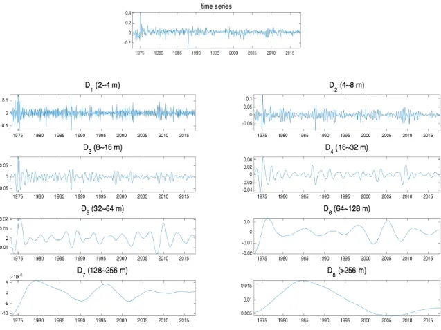
Since we are using monthly data, the first detail component 𝑦_𝑡𝐷1

captures the oscillations between 2 and 4 months, while detail components 𝑦_𝑡𝐷2 _{, 𝑦} 𝑡 𝐷3 _{, 𝑦} 𝑡 𝐷4 _{, 𝑦} 𝑡 𝐷5 _{, 𝑦} 𝑡 𝐷6 _{, 𝑦} 𝑡

𝐷7 _{capture oscillations between 4-8, 8-16, 16-32, 32-64,}

64-128 and 128-256 months respectively. Finally, the smooth component 𝑦_𝑡𝑆7

, now denoted as 𝑦_𝑡𝐷8

, captures the oscillations for a period greater that 256 months.

7 _{Use of Daubechies family of filters can be problematic as they take future data into account (two-sided}

filter), see Murtagh et al (2004), in our analysis this is not a problem because we’ll be doing an expanding window out-of-sample forecast.

To illustrate the decomposition of a time series through MODWT MRA, figure 1 represents the decomposition of United Kingdom´s log stock returns. As expected, the lower the frequency the smoother the filtered time series. We can also observe that this method uncovers new dynamics within the time series that were not originally visible. The sample period runs from 02/1973 to 10/2017.

Figure 1. MODWT MRA decomposition of the stock market return in UK. It is possible to observe

the original time series as well as the eight frequency-specific components (𝐷𝑗) equation (8) in

which the log stock market return is decomposed.

2.2.3 Forecasting with the SOPWAV method

The SOPWAV method differs from the SOP when it comes to forecasting the parts of the market stock returns. While the SOP uses the time series of the different variables, the SOPWAV uses the frequency decomposed time series of the dividend-price ratio, the price multiple growth rate, the denominator of the price multiple growth rate and the seven different predictors that are used to estimate the price multiple in the extended version. The objective in using the frequency decomposed parts is to remove the noise of the time series and use the frequencies that have the highest predictive power. A detailed explanation of the SOPWAV econometric time-series method will be hereby provided, closely following the exposition in Faria and Verona (2018).

Firstly, the maximal overlap discrete wavelet transform multi-resolution analysis (MODWT MRA) decomposition (J=6 and J=7 levels)8 _{is applied to the}

time series of all variables under analysis. For illustrative purposes, using the dp as an example we obtain: dp_t = dp_tD1_{+ dp} t D2 _{+ dp} t D3 _{+ dp} t D4_{+ dp} t D5 _{+ dp} t D6 _{+ dp} t D7_{+ dp} t D8 (9)

As it immediately results from equation (9), one of the characteristics of the MODWT MRA decomposition method is (as opposed to other frequency decomposition methods) the fact that it allows us to preserve the original time series. Since the sum of the components will give us the original series, this allows us to maintain the same information as in a standard time-series analysis.

8_{In this dissertation, as two out-of-sample periods are tested, there are two different J levels (number of}

frequencies that compose the time series) the j=6 level stands for a shorter in-sample period (until 12/1989) and the j=7 level is for the in-sample period until 01/2000.

Secondly, each frequency-decomposed part of the stock market return (dp, gmd and gd) is forecasted separately. The variables dp and gd are forecasted using an AR(1) process and using data only from the components themselves:

dp_t+1Dj = αj+ βjdp_t Dj

+ εt+1 ∀j = 1, … , 8 (10)

gd_t+1Dj = γ_j+ δ_jgd_tDj+ ε_t+1 ∀j = 1, … , 8 , (11)

So that each frequency decomposed part forecast is given by:

E_tdp_t+1Dj = α̂ + β_j ̂ dp_{j t}Dj ∀j = 1, … , 8 (12)

E_tgd_t+1Dj = γ̂ + δ_j ̂ gd_{j t}Dj ∀j = 1, … , 8 , (13)

Where α̂ , βj ̂ , γj ̂ and δj ̂ in equations (12) and (13) are the OLS estimates of αj j , β_j , γj and δj in equations (10) and (11), respectively.

The SOPWAV functions like the SOP in terms of the price multiple usage, so there is a baseline SOPWAV that assumes the price multiple growth as zero and the extended version, in which the multiple´s frequency decomposed parts are forecasted. This is done by running OLS predictive regressions with the frequency component of the gmd as the dependent variable and each frequency component of the different predictors used (represented by x), chosen one at a time, as the independent variable:

𝑔𝑚𝑑_𝑡+1𝐷𝑗 = 𝜂𝑗+ 𝜆𝑗𝑥_𝑡 𝐷𝑗

And then we obtain the forecast of the price multiple growth as:

𝐸_𝑡𝑔𝑚𝑑_𝑡+1𝐷𝑗 = 𝜂̂ + 𝜆_𝑗 ̂ 𝑥_{𝑗 𝑡}𝐷𝑗 ∀𝑗 = 1, … , 8 , (15)

where 𝜂̂ 𝑎𝑛𝑑 𝜆𝑗 ̂ in equation (15) are the OLS estimates of 𝜂𝑗 𝑗 and 𝜆𝑗 in equation (14), respectively.

Thirdly, the forecasts of 𝑑𝑝𝑡+1, 𝑔𝑑𝑡+1 and 𝑔𝑚𝑑𝑡+1 are obtained by summing up the forecasts of their frequency components:

𝐸_𝑡𝑑𝑝_𝑡+1= 𝐸_𝑡𝑑𝑝_𝑡+1𝐷1 _{+ 𝐸} 𝑡𝑑𝑝𝑡+1 𝐷2 _{+ … + 𝐸} 𝑡𝑑𝑝𝑡+1 𝐷8 = ∑8𝑖=1(𝛼̂ + 𝛽𝑖 ̂𝑖𝑑𝑝𝑡 𝐷𝑖_{) (16)} 𝐸_𝑡𝑔𝑑_𝑡+1= 𝐸_𝑡𝑔𝑑_𝑡+1𝐷1 _{+ 𝐸} 𝑡𝑔𝑑𝑡+1 𝐷2 _{+ … + 𝐸} 𝑡𝑔𝑑𝑡+1 𝐷8 = ∑8_𝑖=1(𝛾̂ + 𝛿_𝑖 ̂_𝑖𝑔𝑑_𝑡𝐷𝑖_{) (17)} 𝐸𝑡𝑔𝑚𝑑𝑡+1= 𝐸𝑡𝑔𝑚𝑑𝑡+1 𝐷1 _{+ 𝐸} 𝑡𝑔𝑚𝑑𝑡+1 𝐷2 _{+ … + 𝐸} 𝑡𝑔𝑚𝑑𝑡+1 𝐷8 = ∑8_𝑖=1(𝜂̂ + 𝜆_𝑖 ̂_𝑖𝑥_𝑡𝐷𝑖_{) (18)}

Finally, and following the approach of the SOP method, the forecast of the three parts that compose the stock market returns (dp, gd and gmd) are summed up to obtain the one-step ahead forecast of the stock market returns. For each different predictor x to forecast gmd, the SOPWAV forecasting method is given by: 𝐸_𝑡𝑔𝑚𝑑_𝑡+1= 𝐸_𝑡𝑔𝑚𝑑_𝑡+1𝐷1 _{+ 𝐸} 𝑡𝑔𝑚𝑑𝑡+1 𝐷2 _{+ … + 𝐸} 𝑡𝑔𝑚𝑑𝑡+1 𝐷8 = ∑8𝑖=1(𝜂̂ + 𝜆𝑖 ̂𝑖𝑥𝑡 𝐷𝑖_{) (19)}

In Faria and Verona (2018), the hypothesis of using all the frequencies of each part at the same time was first considered (SOPWAV_ALL), but the results were poor and not statistically relevant.9_{. In order to overcome this issue, Faria and}

Verona (2018) SOPWAV method only considers those frequencies that have the highest predictive power. This is achieved by properly selecting the weights 𝜔𝑖 , 𝜔_𝑖 = {0,1} , in the following equation:

𝐸𝑡𝑟𝑡+1= ∑8𝑖=1𝜔𝑖(𝛼̂ + 𝛽𝑖 ̂𝑖𝑑𝑝𝑡 𝐷_𝑖 ) + ∑8𝑖=1𝜔𝑖+8(𝛾̂ + 𝛿𝑖 ̂𝑖𝑔𝑑𝑡 𝐷_𝑖 ) + ∑8𝑖=1𝜔𝑖+16(𝜂̂ + 𝜆𝑖 ̂𝑖𝑥𝑡 𝐷_𝑖 ), (20)

with weights 𝜔𝑖 being chosen so that they maximize the statistical performance of the predictive model.10

2.2.4. Out-of-sample forecasts

There is in-sample evidence in existing literature (mostly for the U.S stock market) that stock returns contain sufficiently predicting components (Campbell (2000)).

However, Goyal and Welch (2008) showed that all stock returns predictors that performed well in-sample up until then, performed very poorly out-of-sample. By other words, they would not have helped an investor with access only to available information to profitably time the market.

Out-of-sample statistical significance is a very important tool when assessing the model effectiveness, as it demonstrates how the model would have performed during the months within the sample using only the information that

9 _{In this dissertation, the inclusion of all frequencies was also tested in the international markets, but the}

results were also poor and therefore are not presented.

10 _{The statistical performance is measured by the out-of-sample R}

os

2 _{from Campbell and Thompson (2008),}

would have been accessible to an investor. This way, it is generally accepted that predicting models require out-of-sample validation, as Campbell (2008) expressed: “The ultimate test of any predictive model is its out-of-sample performance”.

In this dissertation we are focused on the out-of-sample predictability performance of the models being tested. For robustness reasons we will consider two different out-of-sample periods. We generate one-step-ahead out-of-sample forecasts for stock returns in all the countries under analysis using a sequence of expanding windows. Two different initial samples (from 02/1973 to 12/1989 and from 02/1973 to 01/2000) were used to make the first one-step-ahead out-of-sample forecast (that begins the months after the last in-out-of-sample period). Then the process remains the same until the end of the sample, obtaining a total of 334 ahead forecasts for the 02/1973-12/1989 in-sample period and 213 one-step-ahead forecasts for the 02/1973 to 01/2000 in-sample period. The two out-of-sample periods are therefore from 01/1990 to 10/2017 and from 02/2000 to 10/2017. The popularity of the out-of-sample analysis has to do with the fact that once the forecast begins, the returns that are successively being estimated incorporate all the information from the past (at least from the beginning of the sample) which means that an investor at that time would have been able to carry out the forecast with all the available information that he could possess.

2.2.5 Forecast evaluation

The mean square forecast error (MSFE) is a popular metric for evaluating forecast accuracy, and it is not surprising that MSFE is constantly used in studies of stock return forecastability.

In this investigation the model´s forecasting performance is evaluated using the Campbell and Thomson (2008) out-of-sample R-square (R2os) , which measures the proportional reduction of the mean squared forecast error (MSFE)

for the SOPWAV method in comparison to the same MSFE of a benchmark model (in this case the model using the historical mean, which is the standard benchmark in the literature). The R2os is given by:

R2_{os= 1 −}∑ (rt+1− Etrt+1) 2 T−1 t=t0 ∑T−1t=t0(rt+1− r̅)t 2 , (21) where Etrt+1 is the SOPWAV method stock return forecast for t+1, r̅ is the t

historical mean of stock market returns up to time t, rt+1 is the realized stock market return for the different indexes for t+1, T is the total number of observations in the sample and t0 is the number of observations in the initial sample. From equation (21) results that a positive R2os (negative) means that the model being tested outperforms (underperforms) the benchmark model in terms of MSFE.

As in Ferreira and Santa-Clara (2011) and Faria and Verona (2018), the global statistical significance of the R2os results is addressed in terms of the MSFE-F statistic proposed by McCracken (2007)11_{. The statistical significance test formula}

is hereby presented: MSFE − F = (T − t₀) [∑ (rt+1− r̅)t 2 T−1 t=s0 − ∑ (rt+1− Etrt+1) 2 T−1 t=t0 ∑T−1t=t0(rt+1− Etrt+1)2 ] (22)

11_{We are interested in testing H0: MSFE0 ≤ MSFEi against HA: MSFE0> MSFEi , where MSFE0 is the MSFE}

of the historical mean forecast, while MSFEi is the MSFE of the predictive regression, which corresponds

Chapter 3

Empirical results

3.1. Statistical Performance

In this section we report the results regarding the statistical performance of the SOPWAV method applied in the sample of eight countries under analysis. For comparison purposes we also report the results obtained by the SOP method. Both the SOP and the SOPWAV methods are considered in a specification where only dp and gd are used to forecast stock market returns (the baseline versions), as well as in the extended version where gm is additionally considered. In the following tables it is also reported the selected frequency-specific components (y_tD1 _{to y} t D8 _{or y} t D1 _{to y} t D7₎₁₂

of dp, gd and gmd that maximize the R2os for both of the out-of-sample forecasting periods (02/2000 to 10/2017 and 01/1990 to 10/2017).

As stated in Rapach, Ringgenberg and Zhou (2016), due to the presence of a huge unpredictable component in stock returns, a R2os of approximately 0,5% represents an economically meaningful degree of return predictability

3.1.1. Out-of-sample period: 02/2000 to 10/2017

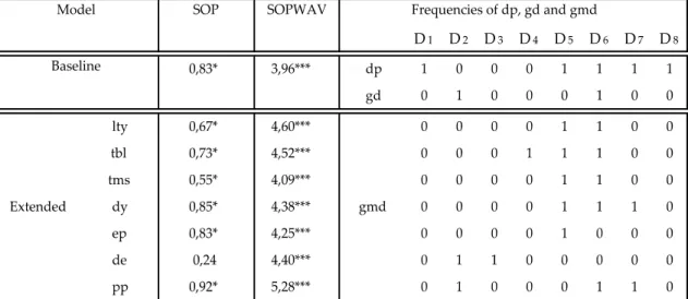
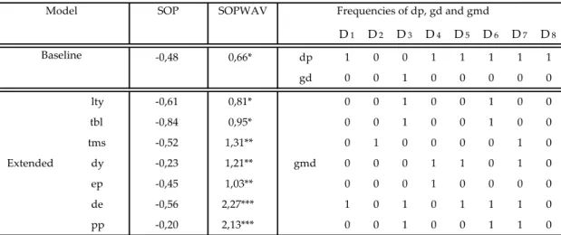
Table 1 reports the results for the statistical performance of the SOP and SOPWAV models for forecasting stock returns in Japan. The frequencies of dp, gd and gmd that maximize the 𝑅𝑜𝑠2 when using the SOPWAV method are also reported. It is immediate to conclude that the SOPWAV method outperforms the SOP both the baseline version and for all extended versions. All the 𝑅𝑜𝑠2 obtained by the SOPWAV models are positive and statistically significance at the 1% level. The higher 𝑅𝑜𝑠2 is 5,28% by using the price pressure to predict gmd. We can also see that the baseline model underperformed the extended version in all its variables.

Table 1. Out-of-sample R-squares (in percentages) for Japan. The sample period is monthly from

02/1973 to 10/2017, and the out-of-sample period under analysis is 02/2000 to 10/2017. Asterisks denote significance of the out-of-sample MSFE-F statistics of McCracken (2007). ***, ** and * denote significance at the 1%, 5% and 10% level, respectively.

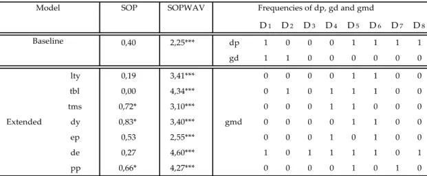
Table 2 provides the results in terms of R2os for the United Kingdom when using the SOP and SOPWAV methods, as well as the frequencies of dp, gd and gmd that maximize the Ros2 . It is possible to verify the effectiveness of the SOPWAV, when comparing to the SOP and also the better performance when using the extended SOPWAV over the baseline version. The variable that better forecasts gmd is the term spread, although all the variables in the extended version perform exceptionally well.

Table 2. Out-of-sample R-squares (in percentages) for the United Kingdom. The sample period

is monthly from 02/1973 to 10/2017, and the out-of-sample period under analysis is 02/2000 to 10/2017. Asterisks denote significance of the out-of-sample MSFE-F statistics of McCracken (2007). ***, ** and * denote significance at the 1%, 5% and 10% level, respectively.

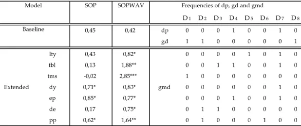
The results for France are presented in Table 3. Again the empirical evidence further reinforces the superior performance of the SOPWAV method versus the original SOP. It is also important to note that the frequency-specific components of gd where not used, which means that for France, the inclusion of gd is not relevant in the model, since its frequencies doesn’t help to increase the 𝑅𝑜𝑠2 .

Table 3. Out-of-sample R-squares (in percentages) for France. The sample period is monthly from

02/1973 to 10/2017, and the out-of-sample period under analysis is 02/2000 to 10/2017. Asterisks denote significance of the out-of-sample MSFE-F statistics of McCracken (2007). ***, ** and * denote significance at the 1%, 5% and 10% level, respectively.

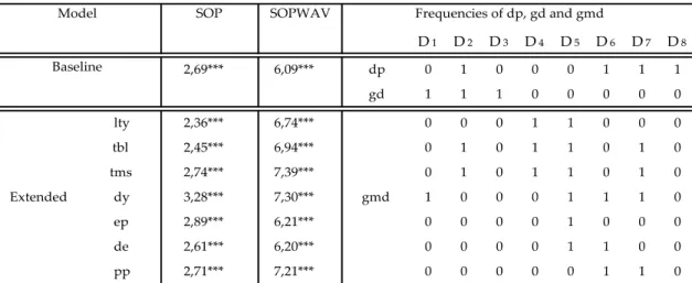
Table 4 exhibits the results for the German stock market. As it happens with the forecasting of French stock market returns, there were no frequency-specific components of gd used to predict stock returns.

Nonetheless, when analysing Germany, we can conclude that the SOP method is not a good method for forecasting its results, because although presenting some positive R2os , none of them proved to be statistical significance at any level. On the contrary, both the baseline and the extended SOPWAV method provided positive 𝑅𝑜𝑠2 , either with 5% or 1% significant depending on the variables.

Table 4. Out-of-sample R-squares (in percentages) for Germany. The sample period is monthly

from 02/1973 to 10/2017, and the out-of-sample period under analysis is 02/2000 to 10/2017. Asterisks denote significance of the out-of-sample MSFE-F statistics of McCracken (2007). ***, ** and * denote significance at the 1%, 5% and 10% level, respectively.

Table 5 display the SOP and SOPWAV statistical performance for the forecasting of Canada´s stock market returns. The 𝑅𝑜𝑠2 for the SOP method are negative in all its versions, which means that a predictive regression based on the historical mean outperforms the SOP method for this stock market. In terms of SOPWAV it is clear that it outperforms the historical mean and SOP method, delivering positive 𝑅𝑜𝑠2 in the baseline and extended versions. Once again the baseline SOPWAV underperformed the extended in all its variables, and the ones that show higher predictive performance are de and pp, that have a statistical significance level of 1%.

Table 5. Out-of-sample R-squares (in percentages) for Canada. The sample period is monthly

from 02/1973 to 10/2017, and the out-of-sample period under analysis is 02/2000 to 10/2017. Asterisks denote significance of the out-of-sample MSFE-F statistics of McCracken (2007). ***, ** and * denote significance at the 1%, 5% and 10% level, respectively.

The results for Switzerland are displayed in Table 6. This is a clear example of the superior ability for the SOPWAV to predict stock returns, with this country being the one for which the SOPWAV methods delivers the highest 𝑅𝑜𝑠2 in the whole sample under analysis (9,45%). This performance is particularly impressive considering that for Switzerland the the SOP method delivers negative 𝑅𝑜𝑠2 in all its forms. Once again it is proved that the inclusion of gmd enhances the ability for the SOPWAV to predict stock returns, as all its variables outperform the baseline version.

Table 6. Out-of-sample R-squares (in percentages) for Switzerland. The sample period is

monthly from 01/1974 to 10/2017, and the out-of-sample period under analysis is 02/2000 to 10/2017. Asterisks denote significance of the out-of-sample MSFE-F statistics of McCracken (2007). ***, ** and * denote significance at the 1%, 5% and 10% level, respectively.

Table 7 reports the results for Australia, where again it is possible to observe the power of the frequency-decomposed components of the stock market returns. All the results for Australia for the SOPWAV (baseline and extended versions) were significant at the 1% level. The variable that better forecasts stock returns is the dividend payout ratio.

Table 7. Out-of-sample R-squares (in percentages) for Australia. The sample period is monthly

from 02/1973 to 10/2017, and the out-of-sample period under analysis is 02/2000 to 10/2017. Asterisks denote significance of the out-of-sample MSFE-F statistics of McCracken (2007). ***, ** and * denote significance at the 1%, 5% and 10% level, respectively.

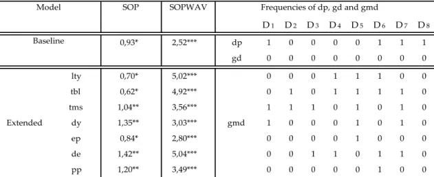
At last, in Table 8 are reported the forecasting results for the South African stock market. This is the market where the statistical performance of the SOPWAV method is less robust. The baseline version delivers results that are not statistically significant. All extended versions of the SOPWAV deliver positive and statistically significant 𝑅𝑜𝑠2 . This performance is globally superior than the one attained by the SOP method.

Overall, results disclosed for the markets under analysis support the strong performance of the SOPWAV model beyond the US market (as reported by Faria and Verona, 2018). There are clear forecasting gains when using frequency-specific components to predict the parts of the stock returns.

It is also curious to observe that across the sample of 8 countries under analysis, the frequencies of dp and gd that in most of the cases maximize the Ros2 are usually the higher (D1 and D2) and the lower (D6 to D8) ones which means that both the dp and gd are useful when predicting higher and lower frequencies of stock market returns. On the other hand, the relevant frequencies of gmd for

Table 8. Out-of-sample R-squares (in percentages) for South Africa. The sample period is

monthly from 02/1973 to 10/2017, and the out-of-sample period under analysis is 02/2000 to 10/2017. Asterisks denote significance of the out-of-sample MSFE-F statistics of McCracken (2007). ***, ** and * denote significance at the 1%, 5% and 10% level, respectively.

forecasting purposes, are generally those from D3 to D6 i.e., this part is helpful for predicting medium frequencies of stock market returns.

This provides valuable insight on the effectiveness of the SOPWAV method, as its components (dp, gd and gmd) follow the dynamics of the effective stock market returns much more efficiently than historical mean or SOP methods.

3.1.2. Out-of-sample period: 01/1990 to 10/2017

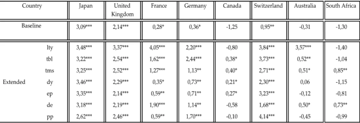
Overall, the results for this forecast period in terms of R2os are worse than the 02/2000 - 10/2017 period even though the SOPWAV still outperforms the SOP in most its variables, and still delivers positive R2os for every country on at least one variable. The results for the SOPWAV performance in this forecast period are presented in Table 9:

As it is possible to see, the SOPWAV keeps its high predictive power for most countries, mainly Japan, United Kingdom, France, Germany and Switzerland, although the results for Canada, Australia and South Africa are not as strong as the out-of-sample period of 02/2000 to 10/2017.

Table 9. Out-of-sample R-squares (in percentage) for the whole sample of countries in the

out-of-sample period of 01/1990 to 10/2017. Asterisks denote significance of the out-out-of-sample MSFE-F statistics of McCracken (2007). ***, ** and * denote significance at the 1%, 5% and 10% level, respectively.