M
arket Anomaly: 2014
thWorld Cup Effect
José Maria Candido Alves
ESCP-Europe Paris (e133401); CLSBE (152413016)
ABSTRACT
Keywords: Behavioral finance, Stock market anomalies, Market efficiency, Investor sentiment,
Flow of information, Abnormal returns, Football
Professor Franck Bancel
Supervisor
“There is a lot of evidence that such overconfidence in intuition is a powerful force in the markets.” Robert J. Shiller
Dissertation submitted in partial fulfillment of requirements for the Double Master Degree Busi-ness, at ESCP-Europe – Paris and Universidade Católica Portuguesa – Lisbon, 2015
Inspired by the World Cup effect discovered by Kaplanski and Levy (2010), we decided to in-vestigate the 2014th edition. Our findings were conclusive. The average return on the U.S. stock market during the latest World Cup was +0.87%, compared to an average of -2.42% of all past World Cups; hence, the anomaly disappeared. We suggest its disappearance was driven by: (1) the growth popularity of Football in the U.S. and its influence on the local stock market, and by (2) the publication of Kaplanski and Levy (2010 and 2014) followed by an investment strategy, which allowed sophisticated investors to take advantage of the anomaly.
Résumé
Inspiré par « l'effet Coupe du Monde » découvert par Kaplanski et Levi (2010), nous avons déci-dé d'enquêter sur la 2014e édition. Nos résultats ont été concluants. Le rendement moyen sur le marché boursier américain au cours de la dernière Coupe du Monde était de + 0,87%, quant à celle de l'ensemble des dernières Coupes du Monde était de -2,42% ; par conséquent, l'anomalie a disparu. Nous avons conclu que ce changement été lié à: (1) la croissance de popularité du football aux Etats-Unis et son influence sur le marché boursier local, et par (2) la publication de Kaplanski et Levi (2010 et 2014) qui a été suivie par une stratégie d'investissement qui a permis aux investisseurs qui étaient au courant de profiter de cette situation.
Mots-clés: La finance comportementale, Anomalies de marché, L'efficacité du marché, Le
senti-ment des investisseurs, Flux d'informations, Les rendesenti-ments anormaux, Le football
Resumo
Inspirado pelo efeito Campeonato do Mundo descoberto por Kaplanski e Levy (2010), decidimos investigar a edição de 2014. Os nossos resultados foram conclusivos; os retornos do NYSE Composite Index durante o Campeonato do Mundo de 2014 foram de +0,87%, em comparação com uma média de -2,42% de todas as edições anteriores, o que faz com que a anomalia tenha desaparecido. Sugerimos como razões para o seu desaparecimento: (1) o crescimento da popula-ridade do futebol nos EUA e a sua influência nos mercados financeiros, e (2) a publicação de Kaplanski e Levy (2010 e 2014) acompanhado de uma estratégia de investimento o que permitiu aos investidores sofisticados tirar vantagem da anomalia.
Palavras-chave: Finanças comportamentais, Anomalias financeiras, Eficiência do mercado
Acknowledgments
In order to successfully complete this chapter I had the invaluable support of amazing people around me, which I would like to dedicate this project.
Firstly, I would like to thank Professor Franck Bancel, my research advisor, for all his support and guidance during this exciting challenge. Additionally, I would like to thank Profes-sor José Faias: for all his support whenever was needed and for preparing me throughout the Empirical Finance course.
Secondly, I would like to deeply thank my parents, who unconditionally supported me throughout this important phase and without whom I would never been able to succeed. The high ethical and hardworking standards they passed me were fundamental and I am deeply grateful for that.
Thirdly, I would like to thank all my closest friends, fellow ESCPs and Católica-Lisbon friends, who helped and supported me to conclude this important chapter.
TABLE OF CONTENTS
I. Introduction ... 1
II. Literature Review ... 2
III. 2014 FIFA World Cup ... 12
IV. Foreign Investment In US ... 14
V. Data ... 18 VI. Methodology ... 20 VII. Results ... 22 VIII. Conclusions ... 36 IX. Appendix ... 37 X. References ... 43
INDEX OF FIGURES
Figure 1 - % of U.S. Equity held by World Cup countries and Foreign Investors in 2014 ... 15
Figure 2 - % of U.S. Equity held by World Cup countries ... 16
Figure 3 - Losing and Eliminated Countries ... 26
Figure 4 - The value of $100 invested during all World Cups ... 27
Figure 5 - The U.S. Stock Market vs. Disappointed Fans ... 30
Figure 6 - Football Popularity in the US ... 31
Figure 7 - Historical MLS Attendance... 32
INDEX OF TABLES
Table 1 - Foreign holdings of U.S. securities by Country ... 17Table 2 - Summary Statistics ... 19
Table 3 - Main Regression results (1950-2014) ... 23
Table 4 - Stock Market Returns and Fans’ disappointment ... 28
Table 5 – Regression of Stock market returns on U.S. Results ... 33
Table 6 – Average Stock Market Returns and U.S. Results ... 34
Table 7 - News from Bloomberg Economic Calendar ... 37
Table 8 - Total Population of World Cup countries ... 39
Table 9 - Main regression results (1950-2006) ... 40
1
I.
INTRODUCTION
I always felt inspired by behavioral finance and its impact on the finance field. In such a prag-matic industry why would exogenous factors, such as weather or sporting events, influence be-havior?
I pursued my interest in this subject matter during the Empirical Finance final project at Católica-Lisbon, which investigated the relation between temperature and stock market returns. Indeed, a statistically significant negative correlation was found. Although there are numerous financial market anomalies, for this investigation I chose to examine the FIFA World Cup effect because it combines two of my passions, football and finance.
When I first read the paper of Guy Kaplanski and Haim Levy (2010 and 2014), I was astonished by their results and posed the questions:
1. What happened during the 2014th FIFA World Cup? 2. If the effect persisted, why did it persist?
3. If not, why and what has changed?
To address these questions, we replicated Kaplanski and Levy (2010 and 2014) analyses for two time periods: (1) from 1950 to 2006, to cross check their results and (2) from 1950 to 2014, to include the latest FIFA World Cup. On top of these analyses, we also hypothesized two reasons for the disappearance of the effect.
The primary goal of this research was to find out if the effect persisted over the 2014th World Cup and what factors were driving this anomaly. Consequently we tested the following hypothe-sis:
1. The U.S. stock market is efficient and therefore there are no abnormal returns. 2. The potential number of disappointed fans affects the stock market returns.
3. The eliminated countries’ direct investment in the U.S. equity market affects the stock market returns.
2
According to our research, the effect disappeared and therefore we complemented our analysis with the following hypothesis, in order to understand the popularity of football before and after the 2010th World Cup:
4. The U.S. national football team results affect the stock market returns.
Our work will be structured the following way: Section I introduces the topic; Section II presents the relevant literature review; Section III and IV report 2014th FIFA World Cup key figures and the impact of foreign direct investment in the U.S., respectively; Section V and VI analyze the data and explain the methodology used, respectively; Section VII presents the results and Section VIII concludes.
II. LITERATURE REVIEW
MARKET EFFICIENCY
DEFINITION
The Efficient Market Hypothesis (EMH) introduced by Fama (1965), which claims that in an efficient market, stock prices fully reflect all the available information. In efficient stock markets, returns are supposed to follow a random walk and investors should expect to obtain an equilibrium rate of return. The random walk hypothesis states that price changes are unpredicta-ble, meaning future returns are not predictable on the basis of past ones. The information con-tained in the past prices is fully and instantly reflected in present prices in an efficient market as argued by Fama (1965). Following his study, many researchers examined the efficiency of capi-tal markets. Since the introduction of EMH (Fama, 1965) researchers have documented several market anomalies in the stock returns.
TYPE OF EFFICIENCY FORMS
There are three forms of market efficiency: weak, semi-strong and strong. Weak form of market efficiency states that current market prices capture all information contained on past
pric-3
es and volume data. Semi-strong, goes further by capturing all publicly available information. Finally, strong form of efficiency states that current market prices reflect not only all publicly available information but also private one.
MARKET ANOMALIES
DEFINITION
Lo (1997) states that researchers have not yet reached a consensus about whether finan-cial markets are efficient or not, in fact it is not the objective of the authors to test that hypothe-sis, but to show evidence of a specific market anomaly during a specific time period – the World Cup Effect.
Reputable scholars such as Richard Roll, Robert Haugen or Paul Samuelson commented the existence of market anomalies and their exploitation. Richard Roll (1994) made it public that
“Over the past decade, I have attempted to exploit many of the seemingly most promising ‘ineffi-ciencies’ by actually trading significant amounts of money (…) Many of these effects are surpris-ingly strong in the reported empirical work, but I have never yet found one that worked in prac-tice.”. Paul Samuelson (1989) recognized that taking advantage of market anomalies before they
being exploited by other players is a challenge that only a few masterminds can have the pleasure to do. He adds that “Out of the thousands of published and unpublished statistical testings of
various forms of the [efficient market] hypothesis, a few dozen representing a minuscule per-centage have isolated profitable exceptions to the theory.” Finally, Robert Haugen (1995) cites
that “In the course of the last 10 years, financial economists have been struggling to explain (…)
the huge, predictable premiums in the cross-section of equity returns”
According to Brennan and Xia (2001), a market anomaly is “the statistically significant
difference between the realized average return (…) and the returns that are predicted by a par-ticular asset pricing model”. Frankfurter and McGoun (2002) defined anomaly as “an irregu-larity or a deviation from common or natural order or an exceptional condition”. In fact,
4
inefficiency. Tversky & Kahneman (1986) defined market anomalies as “an anomaly is a
devia-tion from the presently accepted paradigms that is too widespread to be ignored, too systematic to be dismissed as random error and too fundamental to be accommodated by relaxing the nor-mative system”. In a nutshell and according to financial literature, market anomalies are
de-scribed as uncommon situations in which the movement of a share or a group of shares diverges from the conventions of EMH.
Abnormal returns – actual return minus expected return – are expected to be zero in effi-cient markets, thus persistence realization of those represents an anomaly and consequently translates into predictability of future returns. It is therefore a market distortion that investors have been taking advantage of. However, according to Chordia et al. (2014), the recent policies of liquidity stimulation and lower trading costs made the average returns from a portfolio strate-gy based on anomalies decreased considerably. Furthermore, Schwert (2003) points out that market anomalies tend to attenuate or even disappear after being reported and also that mispric-ing opportunities may not hold for different time periods.
Market anomalies have been identified many years ago and somehow they still persist, but as Hawawini and Keim (1995) argued, there are no “guarantees [of] their presence in the future”. However, there may be numerous reasons for their existence. Firstly, the lack of under-standing of such mispricing might move away investors from investing in such opportunity. Sec-ondly, arbitrage might be too costly due to the bid-ask spread, complexity or transaction costs. Thirdly, the potential profit might be not enough to give it a try, even if the chance exists. Fourthly, the opportunity might be restricted due to trading limitations. Lastly, investors are not always rational and even with new information they might not change their behavior.
According to Latif et al. (2012) market anomalies can be divided into three categories: (1) fundamental, (2) technical and (3) calendar or seasonal anomalies. We created a fourth cate-gory named others for all those anomalies not fitting on the three categories described before.
5
FUNDAMENTAL
- Value anomaly
Graham & Dodd (1934) proved in their research that value stocks outperformed growth stocks. According to their study, value shares perform better than growth ones given its actual growth rate and sales. As proven by Lakonishok et al. (1992), market tends to overestimate growth of the growth stocks and they do it for two reasons: (1) take the wrong conclusions with the existing data and (2) tend to focus too much on past performance, even though there are low probabilities it will occur in the future.
However, both authors agree that institutional investors do not take the wrong conclu-sions but rather have a preference for growth stocks over value, since they were more likely to be the past winners. Lakonishok et al. (1993) adds that this preference is related to the time horizon individuals want their return, which is considerably shorter than institutional investors. Finally, some authors claimed that riskiness was actually the cause for higher performance of value stocks over growth stocks. But, based on other studies (Lakonishok, 2002) value stocks are not riskier when looking at its volatility and beta.
- Low P/E
As identified by Ball and Brown (1968) and Goodman & Peavy (1983), companies with a lower Price to Earnings ratio (PER) were more likely to generate higher future returns and outperform the market while those with a high PER tend to underperform.
- Size effect
The widely known size effect, where small cap stocks tend to outperform larger cap stocks was firstly described by Banz (1981). The author found a higher risk adjusted return for smaller firms since 1941. Such anomaly was even recommended as an investment strategy by Haugen and Lakonishok (1988).
- Book to Market ratio
Chan, Hamao, and Lakonishok (1991) and Fama and French (1992) found that higher book-to-market ratios (the ratio of the book value of a common stock to its book-to-market value) tend to be
asso-6
ciated with higher expected returns. Value effect is well described by Fama and French (1992) and it consists in the creation of portfolios with a long position on stocks with the highest Book-to-Market ratio and a short one on stocks with the lowest Book-Book-to-Market ratio.
- Net Payout Yield
In 1988, Fama and French introduced the dividend yield effect. Stocks with a higher dividend yield generated higher future returns than those with low dividend yields. However, more recent-ly academic studies started to show weakened results and discovered a new effect – Net Payout Yield. Boudoukh et al. (2007) found Net Payout Yield - dividends plus repurchases minus issu-ances – a much stronger predictor of future equity performance than dividend yield. Gray and Vogel (2012) also explored the use of net-debt paydown, which added robustness to the stock-holder metric. A strong argument for the weakening of the dividend yield effect is related with the recent SEC regulation changes.
- Low-volatility anomaly
Ali et al. (2003) study combined the Book-to-market effect with volatility and found that the value effect was greater for stocks with high idiosyncratic return volatility. Baker et al. (2011) also discovered that low volatility stocks consistently outperform high volatility stocks, which was also supported by Dutt et al. (2013). As a supporting argument for the low volatility anoma-ly, the latter study found a strong correlation between low volatility stocks and higher operating returns.
TECHNICAL
- Momentum
Momentum strategies are characterized by a short position on stocks that have declined its value in the past (losers) and long position on firms with recent positive returns (winners). This anoma-ly was firstanoma-ly identified by Jegadeesh and Titman (1993) and later developed by Hons & Tonks (2001), which divided the strategy into two portfolio (loser’s and winner’s) and reported higher returns due to lower risk by the latter then by the former.
7 - Moving Averages
Although technical analyses were in use since the 1800s, Brock et al. (1992) was one of the first studies to show its potential. Moving averages are techniques in which past prices are used in order to predict future prices. They are characterized by mainly two price averages, one long and one short, typical 50 and 15 days respectively. Investors must sell a stock whenever the short average is lower than the longer one and must buy it whenever the short average is above the longer one.
- Trading Range Break
Trading Range Break is another technical analysis studied by Brock et al. (1992), where buy and sell signals are determined by the last 50,150 or 200 days maximum or minimum. An investor would sell a stock if its price falls below a minimum or if it goes above a maximum. Although difficult to implement, the study showed significant and positive returns.
CALENDAR
As Boudreaux (1995) concluded, calendar or seasonal anomalies contradict the weak form of efficiency because it assumes markets can be predicted based on past information. Hence, the existence of such variations contradicts EMH, meaning investors can earn substantial abnormal returns.
- January effect
In 1942, Watchel reported for the first time seasonal effects, in what he recommended a “well
worth watching when formulating an actual investment policy”. Rozeff and Kinney (1976) found
that the average return for the month of January was higher than for any other month in NYSE from 1904 to 1974, which they called the January effect. Few years later, Keim (1983) and Reinganum (1983) claimed that returns for small firms were higher than for larger ones, however disagreed on the reason. Whereas the former argued that this pattern was due to the tax-loss-selling effect, the latter disagreed questioning the true reason for such difference in returns when controlling for size. Lakonishok and Haugen (1987) suggested that the January effect might be due to the window dressing effect, meaning that investors, especially fund managers, sell their
8
poor performers in December in order to hide their losses and buy them back again in January to hold their optimal portfolio structure again.
- Holiday effect
The holiday effect was firstly reported by Lakonishok and Smidt (1988) and showed that half of the positive returns of Dow Jones occurred during the 10 pre-holiday trading days. Cadsby and Ratner (1992) also observed this effect in the US but not in Europe. Ariel (1990) went further and stated that more than one-third of the positive returns in the U.S. occurred on the 8 days be-fore a market closed holiday.
- Day of the week effect
Kelly (1930) found with three years of data that Monday was the worst day to buy stocks. Hirsch (1968) and Cross (1973) drew the same conclusions, but Franck Cross compared Friday average returns with those of Monday. Gibbons and Hess (1981) also compared the first and the last trad-ing days of the week, concludtrad-ing that Friday had higher returns. Another perspective had Jaffe and Westerfield (1989) and Brooks and Persand (2001) reporting Tuesday as the day with the lowest returns for Japan and Australia and for Malaysia and Thailand, respectively.
- Religious effects
Bialkowski et al. (2010) studied the stock market returns during the Muslim Holy Month and discovered that returns were significantly higher and less volatile during this period than the rest of the year. On the other hand, Lakonishok & Smidt (1988) studied stock markets around Christmas time and discovered that “the price increase from the last trading day before
Christ-mas to the end of the year is over 1.5%”. OTHERS
- Neglected Stocks
Neglected Stocks, or Reversals occur when either past top or worst performing stocks reverse and tend to out- or underperform the market in subsequent periods. This event is usually attribut-ed to investors’ expectations of poorly performing stocks to succeattribut-ed and high flyers to fall. An-other common explanation is related to investment fundamentals, i.e. if a stock is performing
9
well, it will become relatively expensive and therefore its valuation will decrease. The same log-ic applies to underperforming stocks. De Bondt & Thaler (1985) studied the event and found that portfolios of prior “losers” consistently outperformed prior “winners”. The authors identified gains of 25% for the past “losers” portfolios compared to those of past “winners” for data ranges as long as 36 months after the creation of the portfolios, which was consistent with their hypoth-esis of markets overreaction. Furthermore, Tversky and Kahneman (1973) argued that a possible reason for such anomaly might be the “excessive pessimism about the future prospects of
compa-nies that had done poorly”.
- Dogs Of The Dow
The Dogs of the Dow anomaly was discovered by John Slatter and involves trading the stocks of the Dow Jones Industrial Average (DJIA). According to this anomaly, an investor who held an equally-weighted portfolio of the ten highest dividend-yielding stocks, for one year, would have an average return of 16.06% versus 10.91% of the overall index. This strategy was particularly successful after the crash of 1987, where the dogs were indeed the underperformers and actually recovered post-crisis. Domian et al. (1998) concluded that the strategy succeeded around the crisis period but weakened afterwards suggesting overreaction as a cause for the success. How-ever, more recently Rinneand Vähämaa (2011) conducted an empirical study of this strategy in the Finnish market and reported average annual abnormal returns of 4.5%.
- Temperature Anomaly
People tend to rate their life satisfactions much higher on sunny days than on cloudy or raining days (Schwartz and Clore, 1983). Evidence suggests that low temperatures tend to cause aggres-sion, and high temperatures tend to cause aggresaggres-sion, hysteria or apathy (Cao and Wei, 2005). According to Saunders (1993) research, less cloud cover is associated with higher returns, and the returns’ difference between the cloudiest days and the least cloudy days is statistically signif-icant. Investors’ mood is upbeat or optimistic on sunny days, which uplifts the stock market re-turns. Conversely, their pessimistic mood on cloudy days depresses the stock rere-turns. Hence, Saunders (1993) as well as Hirshleifer and Shumway (2003) argued that weather can indeed af-fect the behavior of market traders and consequently stock returns. Also, in an empirical study
10
incorporating many weather variables, Howarth and Hoffman (1984) found that humidity, tem-perature and sunshine exercise the greatest influence on mood.
Other studies have tested the impact of ambient temperature alone on mood, behavior and task performance. Allen and Fisher (1978) and Wyndham (1969) found that task-performing abilities are weakened when individuals are exposed to very high or low temperature.
- Daylight Saving Anomaly
Sleeping is crucial in everyone’s life, and even if researchers have been showing its positive ef-fects on productivity and wellness1, stock market participants have been sleeping less. Kamstra’s et al. (2000) analyzed the effect of daylight saving changes on financial markets. His study showed evidence that, weeks following daylight-saving weekends have large negative returns. Kamstra’s argues the effect is related to sleep desynchronosis, which affects negatively sleep patterns.
INVESTOR SENTIMENT
Investor behavior is an important field to which has been devoted increasing attention on capital market studies. Two perspectives have been taking into account: traditional and behavioral fi-nance. Most studies focused on the institutional investors behaviors, due to data availability and impact on the market.
Although, investment behavior has been investigated from the perspective of investment selection decisions, such as the risk-return paradigm, more recent research focused on internal and external behavioral factors. Investment behavior theories attempt to explain the rationality or irrationality behind investment decisions and how they differ among investors, assuming equal amount of information.
1
Dababneh, A. J., Swanson, N., & Shell, R. L. (2001). Impact of added rest breaks on the productivity and well-being of workers. Ergonomics, 44(2), 164-174.
11
Under the EMH, traditional finance theory argues that stock prices fully reflect the in-formation available and all players are rational. However, more recently researchers have been connecting the psychological state of the investors to the markets.
Barber and Odean (2000) disagree that all investors behave rationally, even though mod-ern financial economics defend it. Moreover, investor’s irrational behavior tends to occur more frequently than it was supposed. Behavioral finance includes these conducts into financial mar-ket models. There are mainly two common slip-ups investors make: trade excessively and tend to disproportionately hold on losing investments while selling winners. These authors argue that these deviations come from human psychology. Human beings are naturally over confident and that is the first reason for the bias, while the second is related with the necessity to avoid a regret sentiment.
Therefore, it is well established in the psychological literature that mood, feelings and emotions affect people’s decisions according to Schwartz (1990) and Loewenstein et al. (2001), and that mood itself can be influenced by environmental factors such as weather conditions, con-firmed by Watson (2000).
SPORTING EVENTS
Another equally important part of this study is related with sports and how they impact econo-mies and investors behavior. In fact, the economic impact of sports events is a well-studied sub-ject. Fourie and Santana-Gallego (2011) concluded that countries hosting sports events see an increase of 12.5% on tourist arrivals. Moreover, even those countries that were ready to host one, but lost the bid, still see an increase of 3.4%. Kavetsos and Szymanski (2010) studied the “feelgood” factor around sports events, concluding that “hosting major sporting events raises
reported happiness”, especially for football events. However, they claim this “fellgood” factor is
not systematic and appears to be a short term effect.
This finding is of extreme importance given the existing link reported by Edmans et al. (2007) between mood and stock returns. According to his study, which involved 39 countries and 32 years of data (1973 to 2004), football results are strongly correlated with stock market returns,
12
especially on football losses. Edmans et al (2007) reported “a loss in the World Cup elimination
stage leads to a next-day abnormal stock return of -49 basis points.” On the same topic, Ashton
et al. (2003) measured the impact of the England football team on the FTSE 100 index. The study reported a “statistically significant relationship between the performance of the English
national football team and the exchange in the price of shares traded on the London stock ex-change”. Whitfield (2003) reported that a good result in soccer games affects psychologically
trader’s investment decisions. As an example, when England team was knocked off the 1990 World Cup, the London Stock Exchange fell by 1%. Finally, in Turkey it was proven that foot-ball results affected stock market returns by Berument et al. (2006). Berument observed an in-crease on stock market returns after a victory of Besiktas against its rivals (Fenerbahçe and Ga-latasaray).
III. 2014
THFIFA WORLD CUP
Outside United States of America and Canada, the World Cup is the most important sporting event. Despite the already mentioned effects, the FIFA World Cup has a vast media attention, comparable only to the Olympic Games, with an extensive TV audience, massive merchandise sales and huge attention and involvement by the fans. The 2014th edition was special because it broke numerous records in what concerns television audience. In order to understand its impact, key figures2 are presented below, split into digital exposure (U.S. and Worldwide) and financial impact:
Digital Exposure - US
- All-time record figures in online streaming of matches in the USA
- 2014th World Cup beat TV viewing figures for 2014 NBA Finals and 2013 World Series - “The audience reach in the USA saw a near 20% rise versus that achieved in 2006, with
94.5 million viewers watching some part of the tournament in-home. This is the largest increase in audience reach of any measured market analyzed.”
2
13 Digital Exposure - Worldwide
- 214 countries reached
- 1+ billion people have watched some coverage of the Final game
- All-time high TV viewing records in Germany, the Netherlands and Belgium - The final between GER v ARG attracted the biggest audience in German TV history - Most data ever streamed for an event as fans watch online
- Biggest audience for a TV show in France for 7 years
- Biggest audience for a TV show achieved in UK, Italy, Spain and Portugal for 2 years - The official FIFA app recently became the biggest sports event app of all time with a
rec-ord 28 million downloads.
- 451 million Facebook users were, while FIFA’s Twitter followers surpassed the 16-million mark. The official FIFA World Cup Instagram app increased from 42,000 to 0.8 million followers
- 40+ billion impressions of official FIFA World Cup digital content
Finance
- The tournament will bring an additional R$112.79 billion to the Brazilian economy - Tax revenue for shall amount to as much as USD 7.2 billion3
- According to the Getulio Vargas Foundation, 14 million jobs have been created in the last four years because of the FIFA World Cup, the equivalent of 180 Maracana stadiums filled to capacity
- FIFA invested more than US$ 850 million in the organization of the FIFA World Cup in Brazil
- FIFA staff spent more than 600,000 nights in hotels
- In hotel accommodation in Brazil alone, FIFA and the organizing committee spent more than 500 million reais
3
14
IV. FOREIGN DIRECT INVESTMENT IN THE U.S.
Although soccer popularity has grown exponentially, it still remains as the 4th most popular sport in the U.S., therefore the results of the U.S. national team should not affect directly the stock market, or at least not in the same magnitude as other they do in other countries. Additionally, U.S. stock market is known to be very liquid, which would help in case an investment strategy is put in place. Finally, it is the market where more foreign investors invest.
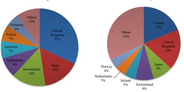
Foreign direct investment in the United States accounted for 16.5%4 of the GDP, which shows the importance of foreign capital in the American economy. On a historical cost basis, totaled $2.8 trillion in 2013, an increase of $0.5 trillion versus 2010, when the last World Cup occurred. United States is the world’s most attractive country in what concerns foreign invest-ment, ahead of China, Russia, Hong Kong and Brazil. However, its share among all foreign di-rect investment dropped from more than 33% in 2000 to less than 20% in 2013, which is a con-sequence of the multinationals expansion for faster growing economies and the competition for foreign investments. From the participating countries, seven of them account for 90% of all Eq-uity held by World Cup countries. As it can be seen in Figure 1, the leading investor is the Unit-ed Kingdom with $741b, followUnit-ed by Japan ($361b) and Switzerland ($331b).
When looking at all countries holding US Equity, Canada is the leader with holdings of almost $770b, followed by United Kingdom and Japan. The seven countries in Panel B represent almost 70% of all US equity held by foreign investors. The “Others” slice aggregates 191 coun-tries and represents $1.3 trillion.
4
15
Figure 1 - % of U.S. Equity held by World Cup countries and by Foreign Investors in 2014
Figure 1 reports the percentage of U.S. equity held by World Cup countries (Panel A) and by all foreign countries (Panel B). On Panel A, 28 countries are reported, being Algeria, Iran and Nigeria the countries without U.S. equity. The other country missing is USA. The “Others” slice corresponds to 21 countries and $223b in investment. Panel B aggregates 198 countries and the “Others” slice corresponds to 191 countries and $1.3t in investment.
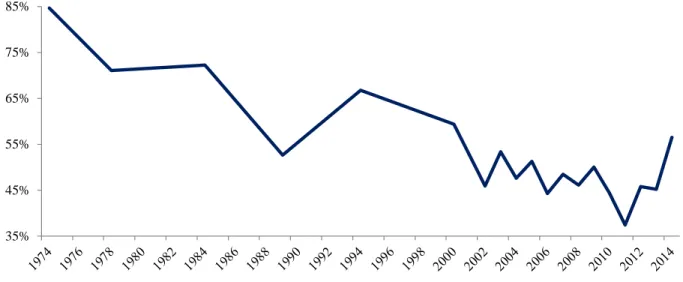
Overall, the 28 teams present in the 2014th FIFA World Cup account for 56% of the all US Equity held by foreign investors in 2014, which represents an increase from 44% in 2010 (Figure 2). Although this percentage is relatively small compared to 1974, where it reached al-most 85%, we need to take into consideration the evolution of the markets and the international investment in rapidly growing economies. The $4.1 trillion of Equity held by foreign investors in 2014 is the maximum since 2002, which by itself proves the importance of such investments for the U.S. economy.
United Kingdom 32% Japan 16% Switzerland 14% Netherlands 8% Australia 7% France 7% Germany 6% Others 10%
Panel A - World Cup countries
Canada 19% United Kingdom 18% Japan 9% Switzerland 8% Ireland 5% Netherlands 5% Norway 4% Others 32%
16
Figure 2 - % of U.S. Equity held by World Cup countries
Figure 2 reports the evolution of the percentage of U.S. Equity held by World Cup Countries since 1974 until 2014.
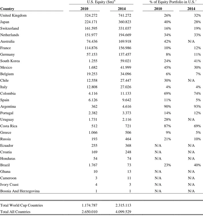
In order to better understand the magnitude of those investments and the share each coun-try allocates to U.S. Equity, Table 1 presents a comparison between the dollar value of U.S. equi-ty held by World Cup countries and the percentage of their equiequi-ty portfolio invested in the Unit-ed States of America in 2010 and 2014. In 2014, the total amount investUnit-ed by foreign investors in the U.S. equity market was about $4.1 trillion, which constitutes an increase of 55% versus 2010. When looking at the countries participating in this World Cup, the value decreases to $2.3 trillion, which constitutes an increase of 97%, when compared to 2010 ($1.1 trillion). About 85% of the participating countries increased their investments in U.S. stocks and more than half allo-cated a higher percentage of their equity portfolio to U.S. securities versus 2010. Thus, a large amount of money is invested in the U.S., and it is reasonable to assume that if part of the portfo-lio is sold, this market will be affected. Finally, about one-fifth5 of the New York Stock Ex-change (NYSE) listed companies are foreign. Hence, foreign investors are familiar with the U.S. stock market and it’s reasonable to assume that a part of them hold a percentage of these compa-nies. Furthermore, most of these companies are listed both in New York and in their country of origin; therefore, even if foreign investors sell their shares in the local market, the U.S. market will be affected otherwise arbitrage opportunities would exist.
5 http://www.world-exchanges.org/statistics/ 35% 45% 55% 65% 75% 85%
17
Table 1 - Foreign holdings of U.S. securities by Country
Table 1 reports the value of foreign holdings of U.S. equity and the percentage of their portfolios invested in the U.S. N/A indicates the data was not available for that country.
U.S. Equity ($m)6 % of Equity Portfolio in U.S.7
Country 2010 2014 2010 2014 United Kingdom 324.272 741.272 26% 32% Japan 224.171 360.823 40% 28% Switzerland 161.595 331.037 16% 19% Netherlands 151.977 194.669 34% 33% Australia 74.436 169.918 42% N/A France 114.876 156.986 10% 12% Germany 57.153 137.457 8% 11% South Korea 1.255 59.021 24% 41% Mexico 1.682 41.999 45% 30% Belgium 19.253 34.096 6% 7% Chile 12.558 27.447 30% N/A Italy 12.808 27.026 4% 4% Colombia 4.116 11.133 69% 74% Spain 6.126 9.642 11% 5% Argentina 362 4.616 90% 93% Portugal 2.382 3.373 14% 12% Uruguay 1.731 2.116 28% N/A Costa Rica 512 721 87% 69% Greece 1.066 506 9% 5% Russia 193 464 21% 10%
Ecuador 255 368 N/A N/A
Croatia 169 248 N/A N/A
Honduras 54 74 N/A N/A
Brazil 1.767 73 23% 40%
Ghana 10 13 N/A N/A
Cameroon 3 11 N/A N/A
Ivory Coast 4 3 N/A N/A
Bosnia And Herzegovina 1 1 N/A N/A
Total World Cup Countries 1.174.787 2.315.113 Total All Countries 2.650.010 4.099.529
6
U.S. Bureau of Economic Analysis, Survey of Current Business (April 2014) - http://www.treasury.gov/resource-center/data-chart-center/tic/Pages/fpis.aspx
7
Coordinated Portfolio Investment Survey (CPIS) data of the International Monetary Fund (IMF) - http://data.imf.org/?sk=B981B4E3-4E58-467E-9B90-9DE0C3367363
18
V.
DATA
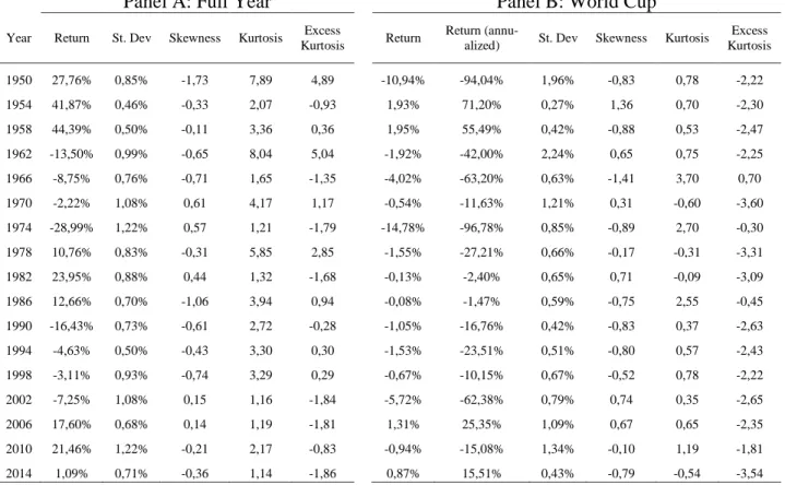
The returns employed on this analysis will be those of NYSE Composite Index, downloaded from Center for Research in Security Prices (CRSP) and the dates will be from January 1st of 1950 to December 31st of 2014. In total there will be 16,443 trading days, from those 255 are EED (Event Effect Days) and 315 are EPED (Event Effect Period Days). The returns considered below are based on an equally weighted portfolio. In Table 2, we present the summary statistics for every World Cup year, divided between the Full Year statistics and the EPED of that year.
As we can see on Panel B, 13 out of 17 World Cups years had a negative return and an annualized rate of return on the World Cup EPED below the rate of return corresponding to the full year (Panel A). The average return for all World Cup periods is -2.23%, whereas the average yearly return is 11.3%, over the same time period (1950-2014).
19
Table 2 - Summary Statistics
Table 2 presents the summary statistics of the sample, which extends from January 1950 until December 2014. There are 17 World Cups r epre-sented. It is divided in two panels: Panel A - Full Year, which compromises all trading days of every World Cup year, and Panel B - World Cup, which refers just to the contest period. Panel A has on average 254 trading days, whereas Panel B has on average 19 trading days. In order to compute the annualized return, the following formula was used: 𝐴𝑛𝑢𝑎𝑙𝑖𝑧𝑒𝑑 𝑅𝑒𝑡𝑢𝑟𝑛𝑛= (1 + 𝑅𝑒𝑡𝑢𝑟𝑛𝑛)(
365
𝑇𝑟𝑎𝑑𝑖𝑛𝑔 𝑑𝑎𝑦𝑠). The market return is the equally-weighted index return from CRSP. Standard deviation = √𝐸((𝑋 − 𝜇)2), Skewness = 𝜎13𝐸((𝑋 − 𝜇)3, Kurtosis =
1
𝜎4𝐸((𝑋 − 𝜇)4 and Excess Kurtosis = 𝜎14𝐸((𝑋 − 𝜇)4− 3 are computed for both panels.
Panel A: Full Year Panel B: World Cup
Year Return St. Dev Skewness Kurtosis Excess
Kurtosis Return
Return
(annu-alized) St. Dev Skewness Kurtosis
Excess Kurtosis 1950 27,76% 0,85% -1,73 7,89 4,89 -10,94% -94,04% 1,96% -0,83 0,78 -2,22 1954 41,87% 0,46% -0,33 2,07 -0,93 1,93% 71,20% 0,27% 1,36 0,70 -2,30 1958 44,39% 0,50% -0,11 3,36 0,36 1,95% 55,49% 0,42% -0,88 0,53 -2,47 1962 -13,50% 0,99% -0,65 8,04 5,04 -1,92% -42,00% 2,24% 0,65 0,75 -2,25 1966 -8,75% 0,76% -0,71 1,65 -1,35 -4,02% -63,20% 0,63% -1,41 3,70 0,70 1970 -2,22% 1,08% 0,61 4,17 1,17 -0,54% -11,63% 1,21% 0,31 -0,60 -3,60 1974 -28,99% 1,22% 0,57 1,21 -1,79 -14,78% -96,78% 0,85% -0,89 2,70 -0,30 1978 10,76% 0,83% -0,31 5,85 2,85 -1,55% -27,21% 0,66% -0,17 -0,31 -3,31 1982 23,95% 0,88% 0,44 1,32 -1,68 -0,13% -2,40% 0,65% 0,71 -0,09 -3,09 1986 12,66% 0,70% -1,06 3,94 0,94 -0,08% -1,47% 0,59% -0,75 2,55 -0,45 1990 -16,43% 0,73% -0,61 2,72 -0,28 -1,05% -16,76% 0,42% -0,83 0,37 -2,63 1994 -4,63% 0,50% -0,43 3,30 0,30 -1,53% -23,51% 0,51% -0,80 0,57 -2,43 1998 -3,11% 0,93% -0,74 3,29 0,29 -0,67% -10,15% 0,67% -0,52 0,78 -2,22 2002 -7,25% 1,08% 0,15 1,16 -1,84 -5,72% -62,38% 0,79% 0,74 0,35 -2,65 2006 17,60% 0,68% 0,14 1,19 -1,81 1,31% 25,35% 1,09% 0,67 0,65 -2,35 2010 21,46% 1,22% -0,21 2,17 -0,83 -0,94% -15,08% 1,34% -0,10 1,19 -1,81 2014 1,09% 0,71% -0,36 1,14 -1,86 0,87% 15,51% 0,43% -0,79 -0,54 -3,54
20
VI. METHODOLOGY
As a matter of coherence the methodology used will be the same as Kaplanski and Levy (2010). The null hypothesis is that the US stock market is efficient and therefore there are no abnormal profits. The alternative hypothesis is that the event coefficient is statistical significant. Regarding the null hypothesis, the methodology used was based on Kamstra et al. (2003) and Edmans et al. (2007) and then ran the following regression:
𝑅𝑡 = 𝛾0+ ∑2𝑖=1𝛾1𝑖𝑅𝑡−𝑖+ ∑𝑖=14 𝛾2𝑖𝐷𝑖𝑡+ 𝛾3𝐻𝑡+ 𝛾4𝑇𝑡+ 𝛾5𝑃𝑡+ 𝛾6𝐸𝑡+ ∑2𝑖=1𝛾7𝑖𝐽𝑖𝑡 + 𝜀𝑡, where 𝑅𝑡 is the daily stock return, 𝛾0is the regression intercept coefficient, 𝑅𝑡−1and 𝑅𝑡−2are the first and second previous day returns, respectively, 𝐷𝑖𝑡 , i = 1..4, are dummy variables for the day of the week: Monday, Tuesday, Wednesday, and Thursday, respectively8, 𝐻𝑡 is a dummy varia-ble for days after a non-weekend holiday9, 𝑇𝑡 is a dummy variable for the first five days of the fiscal year10, 𝑃𝑡 is a dummy variable for the annual event period (June–July), 𝐸𝑡 stands for the event days, and 𝐽𝑖𝑡, i = 1,2, are dummy variables for the 10 days with the highest (i = 1) and low-est (i = 2) returns during the studied period. The variable 𝑃𝑡 is introduced in order to make sure the world cup returns are driven by the event rather than by the specific time of the year (june-july). Likewise, the dummy 𝐽𝑖𝑡 controls for the 10 days with extreme returns (positive and nega-tive).
In terms of the event days, two variables were considered:
a. EED (event effect days) is a game day that is also a trading day and the following day. This definition is based on Edmans et al. (2007) findings that the local effect occurs on the day after the game. I have decided to include the same day of the game as the NYSE was still open after some of the world cup games.
b. EPED (event period effect days) includes all competition days plus break days and two additional trading days. The first EPED is the day of the first game and the last is the day after the final game.
8
Chang, Pinegar, and Ravichandran (1993) and Abraham and Ikenberry (1994) 9
Kim and Park (1994) 10
21
The model will be regressed twice, firstly with an Equally Weighted index from CRSP and secondly with a Value Weighted Index. It is assumed that returns’ volatility is constant. However, according to past literature11 returns have time-varying volatility. To address this is-sue, Kaplanski and Levy (2010) and Edmans et al. (2007) modelled the stock returns using the generalized autoregressive conditional heteroskedasticity GARCH (1,1). The results of the GARCH (1, 1) model didn’t affect their conclusions; therefore, we decided to not include this analysis.
Additionally, we reproduced the following analyses in order to verify the existence of the arbitrage opportunity found by Kaplanski and Levy (2010):
1. Computed returns for the 2014th World Cup and compared them with those of that year. 2. Computed returns for all past World Cup competitions (2014th edition included), starting
in 1950, and compare it with the returns of that year. The objective is to understand if the effect is related with the World Cup or if the year was exceptionally worse than the oth-ers.
3. Compared returns for World Cup years with non-World Cup years, to understand if the effect was driven by a worse than normal World Cup year or if it was directly related with the event. Computed returns for both and conducted a t-test. The null hypothesis that both returns are equal cannot be rejected with a t-value of -1.5612. We also regressed the World Cup (Table 10) years only and compared the results.
4. Since the competition takes place every June or July, we introduced this dummy variable on our regression model to understand if the effect was driven by the months or by the competition itself. We also compared the returns of World Cup years with non-World Cup ones for the month of June and July. The null hypothesis that both returns are equal cannot be rejected with a t-value of 1.9.
11
French, Schwert and Stambaugh (1987) and Bollerslev, Engle and Nelson (1994) 12 𝑡 = 𝜇1−𝜇2
√𝜎12 𝑛1+𝜎22𝑛2
22
VII. RESULTS
In the following section, we will present the regression results for all 17 past World Cups, com-posed by 16,442 trading days, 255 Event Effect Days (EED) and 315 Event Effect Period Days (EPED). Table 3 reports our main regression results. Panel A and B resume the results for EED, whereas C and D resume for EPED. All Panels present regressions on Value-Weighted index (VW) and on Equally-weighted index (EW). The main variable analyzed will be the World Cup days, which assumes the value of EED or EPED.
The main conclusions from our analysis are:
1. The coefficient of the variable World Cup days is negative for all regressions and with high levels of significance, confirming the results of Kaplanski and Levy (2010 and 2014).
2. Our results are robust for all tested variables. This includes the length under analysis (EED and EPED), the model (with and without serial correlation, day of the week, tax year and holiday variables), the index (value- and equal-weighted index) and the most ex-treme positive- and negative-return days.
3. June-July variable is insignificant, meaning the fact that the event occurs during this two months is irrelevant for the World Cup effect.
23
Table 3 - Main Regression results (1950-2014)
Table 3 reports the results of the following regression: 𝑅𝑡= 𝛾0+ ∑2𝑖=1𝛾1𝑖𝑅𝑡−𝑖+ ∑𝑖=14 𝛾2𝑖𝐷𝑖𝑡+ 𝛾3𝐻𝑡+ 𝛾4𝑇𝑡+ 𝛾5𝑃𝑡+ 𝛾6𝐸𝑡+ ∑2𝑖=1𝛾7𝑖𝐽𝑖𝑡+ 𝜀𝑡, where Rt is the daily stock return, γ0is the regression intercept coefficient, Rt-1and Rt-2are the first and second previous day returns, respectively, Dit , i = 1..4, are dummy variables for the day of the week: Monday, Tuesday, Wednesday, and Thursday, respectively, Ht is a dummy variable for days
after a non-weekend holiday, Tt is a dummy variable for the first five days of the fiscal year, Pt is a dummy variable for the annual event period (June–July), Et stands for the event days, and Jit, i = 1,2, are dummy variables for the 10 days with the highest (i = 1) and lowest (i = 2) returns during the studied period. The first line of each test reports the coefficients of the regression and the second line reports the t-values. *, ** and *** indicate a significance level of 10%, 5% and 1%, respectively.
Case Gamma Rt-1 Rt-2
Non weekend
holidays Monday Tuesday Wednesday Thursday
1st 5 days of
Tax Jun-Jul
World Cup
days 10 best days 10 worst days R2
F Panel A - Event Effect Days (EED) - All Game Days
VW
1a - Base model (BM) 0,0008 0,0004 -0,0016 -0,0005 0,0000 -0,0004 0,0007 0,0000 -0,0018 0,005
(5,11***) (0,76) (-7,07***) (-2,01**) (-0,16) (-1,72*) (1,45) (-0,23) (-2,99***) 9,883
2a - BM with serial corre-lation 0,0008 0,0668 -0,0373 0,0003 -0,0016 -0,0004 -0,0001 -0,0004 0,0007 0,0000 -0,0018 0,010 (5,11***) (8,58***) (-4,78***) (0,49) (-7,23***) (-1,64*) (-0,36) (-1,87*) (1,35) (-0,21) (-3,01***) 17,100 3a - BM without control dummy variables 0,0004 -0,0019 0,001 (4,98***) (-3,29***) 10,851 EW 1a - Base model (BM) 0,0014 0,0009 -0,0025 -0,0013 -0,0004 -0,0007 0,0000 -0,0002 -0,0016 0,011 (9,41***) (1,92*) (-11,55***) (-5,96***) (-2,1**) (-3,08***) (0,09) (-1,01) (-2,87***) 22,050 2a - BM with serial
corre-lation 0,0013 0,1526 -0,0112 0,0005 -0,0026 -0,0010 -0,0004 -0,0007 -0,0001 -0,0002 -0,0015 0,033 (8,78***) (19,57***) (-1,44) (0,98) (-12,13***) (-4,67***) (-1,77*) (-3,24***) (-0,14) (-0,81) (-2,73***) 56,568 3a - BM without control dummy variables 0,0005 -0,0019 0,001 (6,97***) (-3,43***) 11,770
Panel B - EED + Extreme Days Dummy Variables
VW
1b - Base model (BM) 0,0008 0,0004 -0,0015 -0,0005 0,0000 -0,0003 0,0007 -0,0001 -0,0018 0,0738 -0,0443 0,102 (5,27***) (0,88) (-6,74***) (-2,33**) (-0,14) (-1,55) (1,52) (-0,49) (-3,11***) (26,92***) (-32,29***) 185,592 2b - BM with serial
corre-lation 0,0008 0,0648 -0,0106 0,0003 -0,0015 -0,0004 0,0000 -0,0004 0,0007 -0,0001 -0,0017 0,0744 -0,0438 0,106 (5,14***) (8,74***) (-1,42) (0,64) (-6,88***) (-1,96**) (-0,19) (-1,66*) (1,39) (-0,45) (-3,07***) (26,92***) (-31,99***) 161,795 3b - BM without control dummy variables 0,0004 -0,0019 0,0736 -0,0446 0,098 (5,38***) (-3,48***) (26,8***) (-32,49***) 595,610 EW 1b - Base model (BM) 0,0014 0,0010 -0,0024 -0,0013 -0,0004 -0,0006 0,0000 -0,0002 -0,0016 0,0791 -0,0445 0,125 (9,85***) (2,11**) (-11,69***) (-6,46***) (-2,21**) (-3***) (0,08) (-1,11) (-3,06***) (30,83***) (-34,71***) 235,733 2b - BM with serial
corre-lation 0,0013 0,1409 0,0168 0,0005 -0,0025 -0,0010 -0,0003 -0,0006 -0,0001 -0,0002 -0,0015 0,0813 -0,0431 0,146 (9,06***) (19,18***) (2,28**) (1,21) (-12,3***) (-5,28***) (-1,66*) (-3,07***) (-0,16) (-0,86) (-2,87***) (31,85***) (-33,9***) 234,055 3b - BM without control dummy variables 0,0005 -0,0019 0,0789 -0,0449 0,116 (7,52***) (-3,66***) (30,6***) (-34,82***) 721,174
24
(continued)
Case Gamma Rt-1 Rt-2
Non weekend
holidays Monday Tuesday Wednesday Thursday
1st 5 days
of Tax Jun-Jul
World Cup
days 10 best days 10 worst days R2
F Panel C - Event Effect Period Days (EPED) - All Game Days + 2 Days
VW 1a - Base model (BM) 0,0008 0,0004 -0,0016 -0,0005 0,0000 -0,0004 0,0008 0,0000 -0,0015 0,005 (5,15***) (0,75) (-7,11***) (-2,03**) (-0,21) (-1,76*) (1,49) (-0,2) (-2,77***) 9,725 2a - BM with serial correlation 0,0008 0,0667 -0,0373 0,0003 -0,0016 -0,0004 -0,0001 -0,0004 0,0007 0,0000 -0,0015 0,010 (5,15***) (8,56***) (-4,79***) (0,49) (-7,27***) (-1,66*) (-0,41) (-1,9*) (1,4) (-0,18) (-2,75***) 16,950 3a - BM without control dummy variables 0,0004 -0,0016 0,001 (4,98***) (-3,02***) 9,137 EW 1a - Base model (BM) 0,0014 0,0009 -0,0025 -0,0013 -0,0005 -0,0007 0,0001 -0,0002 -0,0015 0,011 (9,45***) (1,92*) (-11,59***) (-5,98***) (-2,15**) (-3,12***) (0,12) (-0,89) (-2,9***) 22,075 2a - BM with serial correlation 0,0013 0,1525 -0,0113 0,0005 -0,0026 -0,0010 -0,0004 -0,0007 0,0000 -0,0001 -0,0013 0,033 (8,82***) (19,55***) (-1,45) (0,97) (-12,17***) (-4,69***) (-1,82*) (-3,27***) (-0,1) (-0,74) (-2,63***) 56,512 3a - BM without control dummy variables 0,0005 -0,0017 0,001 (7,01***) (-3,41***) 11,597
Panel D - EPED + Extreme Days Dummy Variables
VW 1b - Base model (BM) 0,0008 0,0004 -0,0015 -0,0005 0,0000 -0,0003 0,0008 -0,0001 -0,0015 0,0738 -0,0443 0,101 (5,32***) (0,87) (-6,78***) (-2,35**) (-0,19) (-1,59) (1,57) (-0,45) (-2,87***) (26,92***) (-32,28***) 185,429 2b - BM with serial correlation 0,0008 0,0647 -0,0107 0,0003 -0,0015 -0,0004 -0,0001 -0,0004 0,0007 -0,0001 -0,0014 0,0744 -0,0438 0,106 (5,18***) (8,72***) (-1,43) (0,63) (-6,92***) (-1,98**) (-0,24) (-1,7*) (1,43) (-0,43) (-2,78***) (26,92***) (-31,98***) 161,632 3b - BM without control dummy variables 0,0004 -0,0016 0,0736 -0,0446 0,098 (5,38***) (-3,2***) (26,8***) (-32,48***) 594,910 EW 1b - Base model (BM) 0,0014 0,0010 -0,0024 -0,0013 -0,0004 -0,0006 0,0001 -0,0002 -0,0015 0,0791 -0,0445 0,125 (9,89***) (2,11**) (-11,74***) (-6,48***) (-2,26**) (-3,04***) (0,12) (-0,99) (-3,09***) (30,83***) (-34,71***) 235,754 2b - BM with serial correlation 0,0013 0,1408 0,0167 0,0005 -0,0025 -0,0010 -0,0003 -0,0006 -0,0001 -0,0001 -0,0013 0,0813 -0,0431 0,146 (9,1***) (19,16***) (2,27**) (1,2) (-12,34***) (-5,3***) (-1,71*) (-3,11***) (-0,13) (-0,8) (-2,74***) (31,85***) (-33,9***) 233,988 3b - BM without control dummy variables 0,0005 -0,0017 0,0789 -0,0449 0,116 (7,55***) (-3,64***) (30,59***) (-34,83***) 721,104
25
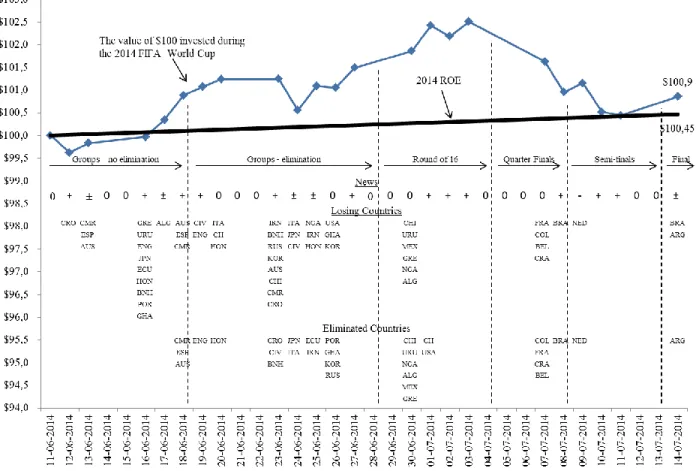
The next step taken was to analyze how a portfolio of $100 performed from the very first day of the 2014 FIFA World Cup until the end of the competition. As it can be seen on Figure 3, and against our hypothesis, the portfolio increased its value throughout the event ending with a value of $100.86 taking into consideration the equally-weighted index. The total return on equity dur-ing 2014 was 0.45%, which means our portfolio had an even better performance durdur-ing the com-petition than it would have if held for the whole year.
On Figure 3, we can also observe a scale of News, which aims to grade the economic news of that day. Classification is divided into: positive economic news (relative to consensus) represented by a “+” sign, negative economic news (relative to consensus) represented by a “–“ sign, inconclusive economic news (if both positive and negative economic news come out) rep-resented by a “±” sign and neutral economic news (if no relevant news are issued on that day) represented by 0. All news are described in detail on Table 7 and were retrieved from Bloomberg Economic Calendar, which reports the main economic and financial news of the day, as well as a consensus scale.
Moreover, two lines are presented: losing and eliminated countries. This information aims to understand how the stock market performed when certain teams lose or are eliminated. There are four interesting insights from this figure: (1) On June 16th, the U.S. national team de-feated Ghana by 2-1, and from that same day stock market rallied until June 22nd; (2) On June 22nd, U.S. sealed a draw against Portugal and the value of our portfolio decreased; (3) On June 26th, U.S. loses against Germany, but advances to the next phase, which is seen as positive and the stock market increases until July 2nd; (4) U.S. is eliminated by Belgium on July 1st and from that time our portfolio depreciates. These findings are coherent with Edmans et al. (2007), where a strong link was found between football results and local equity market. Our hypothesis is that U.S. investors are starting to take a closer attention to football13 and U.S. national team results are affecting the equity market, but this option will be explored further on this research.
13
26
Figure 3 - Losing and Eliminated Countries
Figure 3 presents the value of $100 invested in the NYSE Index during the 2014 World Cup. The bold black line represents a hypothetical in-vestment at the 2014 average return on equity of the whole year. The figure also presents the economic news divided by positive, negative, mixed and inconclusive (+, -, ± and 0, respectively). He second and third line represent the losing countries and the eliminated countries from one stage to the next one.
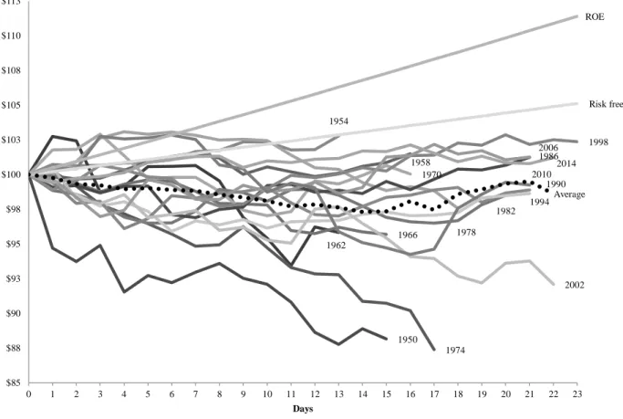
The next step of our analysis was to evaluate the performance of $100 invested in the NYSE Composite Index during the past World Cup Editions and see how they performed. There are 17 World Cup Editions represented and all of them have a performance below a hypothetical investment on a risk free asset or at the average rate of return on equity for the whole period (1950-2014). The 1974th FIFA World Cup Edition was the one where the value of $100 de-creased the most. On the other side, the 1954th edition was the one where the market valued the most. On average, each World Cup has 19 days, being the longest the 1998th (23 days) and the shortest the 1954th and 1962nd edition (13 days).
27
Figure 4 - The value of $100 invested during all World Cups
Figure 4 presents the value of $100 invested in the NYSE Index during all past World Cups. The dotted line represents the average return. The two bold straight lines correspond to the hypothetical investment of $100 at the average rate of return on equity (1950-2014) and the risk free,14 respectively.
In order to understand the possible effect of the disappointment of the fans during the World Cup and its influence on the stock market, we regressed on the returns of our portfolio two variables: (1) the accumulated percentage of population from the countries eliminated from the World Cup and (2) the accumulated percentage of investment in U.S. equity by countries eliminated from the World Cup.
Starting with the NEWS dummy variable, we concluded that they are insignificant, but we need to consider that only a small sample was tested. Surprisingly and contrarily to what Kaplan-ski and Levy (2014) found, the variable DISAPPOINTMENT is positively correlated with the returns of our portfolio with a high significance level. Our hypothesis is that this variable has lost strength compared to the last World Cup edition since it doesn’t seem logical that the less 14 http://pages.stern.nyu.edu/~adamodar/New_Home_Page/datafile/histretSP.html 1950 1954 1958 1962 1966 1970 1974 1978 1982 1986 1990 1994 1998 2002 2006 2010 2014 Risk free ROE Average $85 $88 $90 $93 $95 $98 $100 $103 $105 $108 $110 $113 0 1 2 3 4 5 6 7 8 9 10 11 12 13 14 15 16 17 18 19 20 21 22 23 Days
28
lation and investment in the U.S. the better the performance, although it is highly significant. According to our results, the FINALS dummy variable had a negative correlation with our portfo-lio performance, which can be easily verified on Figure 5 This finding is according to our expec-tations, since neither the NEWS nor the DISAPPOINTMENT could explain this performance, and they were already included in the model. Taking into consideration the Durbin-Watson test, the series seems to be inconclusive regarding autocorrelation.
Table 4 - Stock Market Returns and Fans’ disappointment
Table 4 reports the results of the following regression:
𝑆𝑇𝑂𝐶𝐾𝑇= 𝛽0+ 𝛽1𝑁𝐸𝑊𝑆𝑇+ 𝛽2𝐷𝐼𝑆𝐴𝑃𝑃𝑂𝐼𝑁𝑇𝑀𝐸𝑁𝑇𝑇+ 𝛽3𝐹𝐼𝑁𝐴𝐿𝑆𝑇+ 𝛽4𝑆𝑇𝑂𝐶𝐾𝑇−1+ 𝜀𝑇,
where the variable STOCKt denotes the value in day t of $100 invested in the NYSE Composite Index during the 2014 World Cup; NEWSt is
equal to −1, 0 or 1 depending on whether the economic news in day t was negative, inconclusive or positive, respectively; DISAPPOINTMENTt
is one of the fans’ disappointment variables: a) The accumulated percentage of the population corresponding to countries eliminated from the World Cup, which serves as a proxy for the potential number of disappointed fans; b) The accumulated percentage of investments in U.S. equities corresponding to countries eliminated from the World Cup, which serves as an indicator for the potential effect of the disappointed fans on the U.S. stock market; and FINALSt is a dummy variable corresponding to the Finals Period, which serves as a control variable to understand the
decline during this period. The first line of each test reports the regression coefficients and the second line reports the corresponding standard errors’ t-values (in brackets). * indicates a significance level of 5%. ** indicates a significance level of 1%.
Disappointment variable Constant News Disappointment Finals Stock -1 R2 DW Potential number of disappointed fans 41,60 -0,10 0,99 -0,73 0,59 0,74 2,81
(2,49*) (-0,67) (2,25*) (-2,39*) (3,52**)
Eliminated countries' foreign direct investment in the U.S. 58,47 0,03 1,27 -0,61 0,42 0,74 2,84 (2,75**) (0,16) (2,34*) (-2,31*) (1,95)
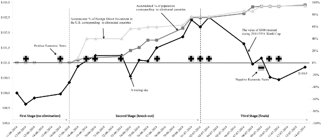
During the first stage, the negative sentiment was relatively small, since teams were not eliminated and even those who lost still had a chance to proceed to the next phase. Thus, the in-crease in price can be attributed to the positive economic news released on June 12th and on June 16th. On the first part of the second stage, market prices remained stable, which was not coherent with the positive economic news and with the increased percentage of foreign direct investment in U.S. corresponding to eliminated countries. However, on June 26th, the price dipped, which can only be explained by an abrupt increase on the accumulated percentage of population and foreign direct investment by eliminated countries. From then on the value of our portfolio in-creased steadily until the beginning of the third stage. An alternative explanation for the sharp increase at the beginning is the fact that sophisticated investors, who did not enjoy the full poten-tial of the anomaly in 2010, bought stocks earlier which increased the market prices. During the final phase, a consistent depression on the value of our portfolio can be seen potentially
motivat-29
ed by the negative sentiment. However, the positive economic news released during this period contradicts this movement. Finally, the inflection observed on July 11th of 2014 was very similar to the one of 2010, which we argue was caused by investors’ expectation in a market rebound driving prices up.
As we can observe on Figure 5, during the 2014th FIFA World Cup the disappointment variables were positively correlated with the performance of the stock market, which contradicts the negative sentiment effect defended by Edmans et al. (2007) and further confirmed by Kaplanski and Levy (2010 and 2014). During the first and second stages of the event, the portfo-lio appreciated, on average, whereas during the final stage it depressed.
30
Figure 5 - The U.S. Stock Market vs. Disappointed Fans
Figure 5 juxtaposes the value of $100 invested in the NYSE Composite Index on the accumulated percentage of foreign direct investment in the U.S. corresponding to eliminated countries and the accumulated percentage of population corresponding to eliminated countries. It also presents the positive and negative relevant economic news.
31
Contrarily to past World Cup editions, the return of an equally-weighted portfolio on the NYSE Composite Index during the 2014th edition was positive and above the stock market return of that year. Thus, the World Cup effect Kaplanski and Levy discovered in 2010 may have van-ished. We propose two hypotheses for such disappearance:
1) Football popularity growth and US national team results
American football has been always the most popular sport in the U.S., seconded by bas-ketball and baseball. These three sports account for 62% of all mentions and therefore take the lead. Historically, the “battle” between Racing, Hockey and Football has been tight, with Racing being the fourth, Football the fifth and Hockey the sixth. However, since the last World Cup in 2010 this trend has changed considerably and U.S. has now more “Soccer” fans than any time in the last 20 years, as it can be seen on Figure 6. Despite it only got about 8% of the choices, pref-erence is worth as much as Hockey and Racing together and therefore its influence on financial markets might be much higher than it was during the last World Cups.
Figure 6 - Football Popularity in the US15
Figure 6 reports the evolution of popularity among Football, Hockey and Racing from 1994 until 2013. The red dotted circle indicates the mo-ment when football surpassed Hockey in popularity.
In order to prove this increasing popularity, we also investigated the Major League Soc-cer (MLS) attendance, as it is a decent proxy for the interest in Football. On Figure 7, we can observe that from 1996 until 2002, the number of football supporters remained relatively stable 15 http://www.sportsbusinessdaily.com/Journal/Issues/2014/01/06/Research-and-Ratings/Up-Next.aspx - accessed on April 29th Racing Football Hockey 2 3 4 5 6 7 8 1994 1995 1996 1997 1998 1999 2000 2001 2002 2003 2004 2005 2006 2007 2008 2009 2010 2011 2012 2013 P o p u la rit y ( % )
32
at an average of 2.5m. However, since 2002 this number increased considerably reaching the 4m annually spectators. From 2010 onwards, the MLS attendance increased 55% to more than 6m annual spectators, which corresponds to an increase of 100% vs. 2002. An important contributor to this statistic was the arrival of many renowned players such as David Beckham (2007), Thier-ry HenThier-ry (2010) and Kaká (2014).
Figure 7 - Historical MLS Attendance
Figure 7 reports the evolution of the MLS attendance from 1996 until 2014.
Furthermore, to prove our hypothesis that football has increased its influence on the U.S. equity market, we decided to regress all results of the U.S. national team on the returns of the NYSE Composite Index equally weighted. Our regression is the following:
𝑅𝑡= 𝛾0+ 𝛾2𝐺𝑎𝑚𝑒𝐷𝑎𝑦𝑡+ 𝛾3𝑅𝑒𝑠𝑢𝑙𝑡𝑠 + 𝜀𝑡,
where Rt represents the return of NYSE Composite Index equally weighted taken from CRSP; GameDay is a dummy variable, which takes the values of 1, if a game occurred on that day or on
the day before, or 0, if no games occur on that day and Results16, which assumes the value 1 for a victory of U.S. National Team, -1 for a defeat or a draw17 and 0, if no games are played.
According to our research, returns are positively correlated with football Results after the 2010th FIFA World Cup, which means there might exist a link between victories and positive market returns and therefore football results are starting to have an influence on the U.S. equity market. On the other side, before the 2010th World Cup, our results were mixed, hence no conclusion can be drawn. It is important to mention that the Results coefficients were not significant. We could also observe that the GameDay variable had a negative coefficient, which means every time the U.S. National team played the stock market returns were negative. This result was highly significant and would require further research.
16
http://www.socceroverthere.com/?page_id=11524 17
The reference point of a football fans is that their team will win (also known as fans’ “allegiance bias”) and there-fore a draw would be a negative result.
2.000.000 3.000.000 4.000.000 5.000.000 6.000.000 7.000.000 1996 1997 1998 1999 2000 2001 2002 2003 2004 2005 2006 2007 2008 2009 2010 2011 2012 2013 2014