The determinants of housing prices in Portugal between 2000 and 2015

(1)

i

The determinants of Housing Prices in

Portugal between 2000 and 2015

Manuel Proença Varão

Dissertation written under the supervision of João César das Neves

Dissertation submitted in partial fulfilment of requirements for the MSc in

Strategy and Entrepreneurship, at the Universidade Católica Portuguesa,

(2)

ii

Abstract

The main purpose of this thesis is to study the impact of demand, political and structural shocks on the housing prices in Portugal between 2000 and 2015. This dissertation is inspired in a paper authored by Dan Andrews (2010) who did a similar research for OECD countries between 1980 and 2005. The period in analysis was a very sensible one for Portugal due to the economic crisis. Regarding the Real Estate, after a decade (90’s) of persistent-housing-price increase, there started a natural adjustment in 2000, reaching its minimum in 2013 (at the end of the economic crisis).

Anyway, and similarly to what the OECD paper did, the variable impacts on housing prices through econometric regressions have been estimated. Due to the economic crisis mentioned above, it is to be noted that these regressions as well as the direct comparisons with the OECD were tricky. However, it was possible to come to some conclusion. On the one hand the demographic shocks were proven as the most relevant - an increase in population, either through an increase in immigration or in birth rates, affects housing prices positively - confirming the expected result. This increase is explained by an increase in the demand for housing and consequently in prices, especially if the Supply takes too long to adjust. On the other hand, the political and structural shocks were inconclusive in this dissertation either because they were not significant in the regressions or the impacts estimated were opposite to what was expected.

Keywords: Real Estate, Housing Prices, Portugal, Demographic shocks, Structural Shocks, Policy Shocks, Economic crisis

Sumário Executivo

A presente tese procura estudar o impacto da procura, das decisões políticas e das decisões estruturais no preço das casas em Portugal entre 2000 e 2015. Esta dissertação é inspirada numa publicação da autoria de Dan Andrews (2010) que fez uma investigação idêntica para os países da OCDE entre 1980 e 2005. O período em análise foi um período bastante sensível para Portugal devido à crise económica. Em relação ao Imobiliário, depois de uma década (anos 90) de crescimento persistente dos preços, iniciou-se um ajustamento natural a partir do ano 2000, atingindo o mínimo em 2013 (final da crise económica).

Os impactos das variáveis em análise no preço das casas foram estimados através de regressões econométricas, à semelhança do que foi feito na publicação da OCDE. No entanto, devido à crise económica mencionada acima, as regressões e as comparações diretas com a publicação que serviu como inspiração tornaram-se traiçoeiras. Apesar de tudo foi possível chegar a algumas conclusões. Por um lado, os impactos demográficos demonstraram ser os mais relevantes – um aumento da população, seja através de um aumento da imigração ou das taxas de natalidade, afetam o preço das casas positivamente – confirmando o esperado. Este aumento é explicado por um consequente aumento da procura de habitação (afetando os preços), especialmente se a oferta demorar muito tempo a ajustar. Por outro lado, os impactos políticos e estruturais foram inconclusivos na tese seja por não serem significantes nas regressões ou porque os impactos estimados foram o oposto do que era esperado.

Palavras-Chave: Imobiliário, Preço Habitação, Portugal, impactos Demográficos, impactos Estruturais, impactos Políticos, Crise Económica

(3)

iii Obrigado aos pais, avós, irmãos e Jéssica. Um Obrigado especial à Avó Lena, Avô António

(4)

iv Index 1. Introduction ... 1 1.1. Topic presentation ... 1 1.2. Problem Statement ... 2 1.3. Research Question ... 3 1.4. Methodology ... 4 2. Literature Review ... 7

2.1. Real estate determinants ... 7

2.2. Portuguese Case ... 10

3. Real House Prices ... 13

3.1. Demand Shocks ... 13

3.1.1. Mortgage market deregulation ... 14

3.1.2. Labor market Shocks ... 14

3.1.3. Demographic Shocks ... 15

3.2. Identification Framework ... 16

3.2.1 Econometric model of the OECD paper ... 16

3.2.2 Adapted econometric models ... 17

3.3. Data ... 18 3.4. Regressions ... 19 3.4.1 Univariate ... 19 3.4.2 Bivariate ... 27 3.4.3 Multivariate ... 31 4. Conclusion ... 33 5. Bibliography ... 35 6. Attachments ... 38

(5)

v Table Index

Table 1: Univariate model with Net-Migration ... 20

Table 2: Univariate model with NAIRU ... 21

Table 3: Univariate model with Interest ... 22

Table 4: Univariate model with Income ... 23

Table 5: Univariate model with Construction Costs ... 24

Table 6: Univariate model with Inflation ... 26

Table 7: Univariate model resume ... 27

Table 8: Bivariate model with NAIRU and Migration ... 28

Table 9: Bivariate model with Construction Costs and Migration ... 29

Table 10: Bivariate model with NAIRU and Construction Costs ... 30

Table 11: Bivariate models resume ... 30

Table 12: Bivariate model with Construction Costs, NAIRU and Migration. ... 31

Graph Index Graph 1: Real Housing Prices Index. 2015 - 100 ... 3

(6)

1 1. Introduction

1.1. Topic presentation

When choosing a topic for this thesis some drivers would have to be considered.

It would have to be related to some content learnt in the Master Studies and above all it would have to be about some subject considered appealing, useful and up to date.

The real estate was one of the topics being more and more dealt with in the international agenda especially after the Subprime crisis in the United States of America in 2007 and all the impacts that it had on many economies.

That was appealing and so the topic for this thesis would be the evolution of real estate in Portugal in recent years.

As an inspiration, a paper published by the OECD - Organization for Economic Co-Operation and Development – entitled “Real House Prices in OECD countries” authored by Dan Andrews will be used. This paper will serve as an important theoretical support. The ideal would be to replicate it for the Portuguese Economy however some adjustments will have to be made. The OECD paper will be better explained below in the section Methodology (chapter 1.4).

This topic was considered useful and up to date once all of us at some period in our lives, sooner or later, do need to have contacts with real estate, as everyone needs to buy a house to sleep, to live or eat. Moreover, there are lots of jobs directly related to real estate, as the case of architects, builders, engineers, developers, investors and facility managers.

Using the R-Language and the statistical knowledge learnt and used in Business Research Methods course will be the way to connect it with the content learnt in the Master. This software (R-Studio) is essential to process and analyze the data. It will be used to build and to estimate the econometric models. The advantage of using this specific software to the detriment of others like, for example, SPSS is the fact that it is computer and user-friendly. This will improve some capacities to use R, which will also potentially be very useful in a future professional life.

(7)

2 has proved an exceptional case in respect of residential property, with house prices mired in stagnation while in other countries they have skyrocketed.” Milleker (2006). “In the residential sector we are facing one of the best moments of the market, watching a total renovation of Lisbon and Porto’s cities” JLL (2015).page For several economies “housing is the most important form of savings for many households.” Fand and Peng (2003).

The relevance of the topic is also reflected in statistical numbers. According to the numbers of

INE (Instituto Nacional de Estatística) in the period before the economic crisis in 2007, on

average 65% of the loans in Portugal were directly related to real estate. Nowadays it is already recovering but the minimum was in the middle of 2012 - 12.5% -. The annual number of real estate deeds in Portugal was around 600 000 before the crisis and today it is about 250 000 (the minimum was around 140 000 in 2012 – which corresponds to a fall of 77% in just a few years). JLL, a reputed real estate consulting firm, announced that in 2017 the investment in real estate ascended to 1 900 million euros (an increase of 50% compared with the previous year). All these numbers reflect the real estate relevance for the economy.

1.2. Problem Statement

In this small section, the aim is to explain the reasons to be interested in Real Estate.

The real estate topic is something transversal to the society, everyone needs a house to live, to eat and to sleep as stated before. Furthermore, it is increasingly seen as a good investment opportunity, either as a personal or as a professional investment.

However, in recent years, there has been some discussion about the housing prices fluctuations and how they are being affected by Demographic, Structural and Policy factors. Are they unreasonably high? Or are they just adjusting to an increase in demand mainly due to the boom of tourism? Are the housing prices adjusted to the Portuguese salaries? The next chart is an Index representing the real house prices (adjusted to 2015 – equal to 100) for Portugal between 1990 and 2017.

(8)

3 Regardless of the answers, the truth is that there has been a movement from households living in city centers (mainly Lisbon and Porto) to the outskirts due to the high cost of living in the centers.

Consequently, understanding these fluctuations and how they vary with macroeconomic cycles maybe useful to eliminate some uncertainty about price evolution as well as understanding what measures can be taken to better control the evolution of prices.

1.3. Research Question

The main objective is to analyze the role of demand shocks and structural and policy factors1 in the housing prices in Portugal, between 2000 and 2015, using the OECD paper as a guideline. As explained before, that paper will be the basis for this work and econometrics will be used to assess the role of each one of these factors.

It will also be considered whether Portugal is affected in the same way as the other countries and, if necessary, it some other issues will be investigated as the analysis is being made in a

1_{As will be explained further, in this dissertation Migration, NAIRU, Construction Costs, Inflation, Interest Rate} and Average Disposable Income will be the demand, policy and structural factors in analysis.

(9)

4 different period from the period the original paper is analysing.

Based on all this information the Research Question was formulated.

What is the impact of the demand shocks, the structural and the policy factors on the real housing prices in Portugal, from the period of 2000 to 2015?

This is the crucial question. Firstly, this is what is relevant when trying to find out when replicating the paper for Portugal. Therefore, throughout the essay there will be a strong focus on this question trying to find not only the real price of housing but also the clear effect that each one of these factors has on the prices. This effect will be measured through correlations, using an econometric model and the R-language.

Secondly, is Portugal a country like the OECD prototype as presented in the paper in terms of how prices are influenced by several factors? This question is important for the analysis to write the thesis. Though not crucial yet it would be useful to know if Portugal behaves in a similar way as other countries do. The way this will be answered is by confronting the conclusions of this thesis with the ones in the paper.

Thirdly, must some other issues be taken into consideration when analysing a period different from the one originally analysed in the paper? This question although not the centre of the thesis, is important once the two periods are somewhat different. In between them, there was a huge crisis that changed the way some people/countries/institutions look at the market itself. Therefore, the environment to do a trustable analysis will have to be adapted.

1.4. Methodology

As mentioned above a paper published by the OECD - Organization for Economic Co-Operation and Development – entitled “Real House Prices in OECD countries” authored by Dan Andrews as an inspiration will be used.

Some specific factors are referred to in the paper as affecting the housing prices:

(10)

5  Structural factors – influence the price though not resulting from the policy maker’s

will;

 Policy factors – influence the price resulting from the policy maker’s action.

The paper used an econometric model and its aim is to explain the real price of housing and how it is affected by the variables of the model.

The variables included in the model are: Interest Rate, Migration, NAIRU - Non-Accelerating Inflation Rate of Unemployment, Average Disposable Income, Bank Regulation, Construction Costs, Dwelling Stock, Population Evolution and Inflation.

The first big conclusion that the paper presents is the fact that the structural factors have an indirect rather than a direct effect on the housing prices. This means that its effect is observed through the demand impacts. As Andrews (2010) defends “the impact of structural factors is identified indirectly through their interaction with demand shocks”.

First of all, this paper has been chosen because it is about the topic to be investigated in this thesis, secondly because it is from a trusted and very well reputed source (OECD) and thirdly because it applies theoretical contents as learnt to do in the Master Studies to an appealing topic.

The period to be taken into consideration in this thesis will be different from the one in the original paper. While it analyzed the years between 1980 and 2005 here the period from 2000 to 2015 will be analyzed.

In what concerns the sample, the original one is about all the OECD countries, however just one country – Portugal – will be taken into consideration. Considering a shorter period of time and a much shorter sample the econometric model will have to be adapted, (if the same as in the paper was used it would be obviously very significant) however it will be explained throughout the thesis.

Regarding the data, the main sources to be used will be from reputed institutions: OECD Economic Outlook, INE (Instituto Nacional de Estatística), Banco de Portugal and PORDATA.

The housing prices (dependent variable data), that will be used in the regressions, are an index of the real prices having the basis year 2015 equal do 100. The source of this Index is the OECD

(11)

6 Economic Outlook (the data basis is roughly the same of the OECD paper). In the attachments, the average prices (€/sqm) verified in December of each year (from 2005 to 2015) are shown. Further on, they will be better explained.

To develop the thesis, the focus will be more on secondary rather than primary data2_{. This} means that an observational study will be the option. The surveys are not believed to make sense here once a behavior or psychological factors are not being tested/studied but how an entire industry is affected by macro-economic policies. Both qualitative and quantitative data will be used in this analysis. In short, through the information obtained from the sources, the correlations between the several variables and between each one of them with the price of housing will be made. This will help understand how each one of them affects the price.

The advantages of using secondary data in this specific case are clear. The first one is the fact that information from the past will be used (prices of houses, number of mortgages, value of mortgages and evolution of interest rates) as there is no alternative but get them from secondary sources. Secondly due to the big number of observations (houses) it will be very difficult to get the values needed of all the houses. Thirdly, it would be tremendously costly (not only in time but in money as well) to do it.

As explained above the R-Studio will be essential to systematize the secondary data collected from the sources and to generate the econometric models.

2_{Primary data is data directly collected by the investigator while secondary data is collected from already}

(12)

7 2. Literature Review

Before just starting with the development of the topic, it was thought to be advisable, valuable and worth getting some experts’ views not only about the variables affecting housing prices but obtaining a brief view about Portugal (in economic/political terms) as well. This will help to easily understand the topic.

2.1. Real estate determinants

Andrews (2010) approaches the topic writing “differences in supply conditions are important since they determine the extent to which increases in demand for housing results in higher prices”. Although this seems trivial knowledge (interactions between demand and supply that determine the price) it may be considered as a good remark to understand the real estate industry namely in countries where supply has been constrained for a long time.

The importance Andrews gives to the supply is based on the construction sector features. If it takes too long to react to an increase in demand, this will result in higher prices (at least in the short run). The quality of the construction also plays a role. In general low quality construction is faster to build (wood houses, for example), which means that an increase in demand will have a minor impact on prices. This explains why in markets where the construction sector is close to its maximum capacity very often the adjustment occurs through an increase in price rather than an increase in the supply itself (Gyourko, 2009). The volatility of the housing prices also depends on the supply responsiveness to large demand shocks. (Catte et al. 2004).

Ozanne and Thibodeau (1983) showed that a great proportion of the housing prices volatility in metropolitan areas could be explained by fundamental economic variables where housing markets are based: the size of the market, consumer characteristics (household income, preferences and expectations), and housing production variables (operating and capital costs, land prices and geographic and government growth constraints). The analysis of this thesis below will determine which pattern the Portuguese case fits into.

More than a decade ago, Capozza, Hendershott and Mack (2004) did some investigation on housing price dynamics. Miller, Sklarz and Thibodeau (2005) wrote about their study whose aim was to explore “patterns of serial correlation in house prices, the notion of mean reversion (towards what we call intrinsic value) as well as how fundamental demand and supply variables

(13)

8 (measuring information dissemination, supply costs and expectations) influence house prices”. Capozza, Hendershott and Mack (2004) came to two main conclusions.

The first one was the fact that contemporaneous house prices are considerably different from the long-run equilibrium prices.

The second one was that serial correlation (in housing prices) is associated with high real construction costs, rapid population growth and real income growth. In the Portuguese case the delay between actual prices and long-run equilibrium price in detail will not be considered. However the importance given to the construction costs, population growth and real income growth must be highlighted.

In what regards inflation, there are some studies that lead to different, but well supported, views about how it affects the housing prices. Two of them will be mentioned.

On the one hand Feldstein (1992) stated that inflation may reduce people’s incentive to invest in real estate which in turn lowers housing demand (affecting prices negatively). Increased prices diminish the value of real wealth, which diminishes demand.

On the other hand, Kuang and Liu (2015) indicated that “the theoretical model demonstrates that house prices and inflation are positively correlated and endogenously determined” which is the opposite view.

Hence, it may be concluded that external conditions could also play an important role on how inflation affects prices. This dissertation will attempt to ascertain the degree of this correlation.

To analyze the impact of income on the housing prices, Xu (2016) considers that it is important to enhance that housing, as an investment, is different from investing in stocks, bonds or funds which means that there will be a different correlation with the disposable income. This happens because housing can also be seen as a consumer good. Accordingly, Xu (2016) said that “income increases result in stimulation for people to improve their living conditions or climb the property ladder and thus drive demand for larger homes, thus putting greater strain on the available space or properties”. As mentioned above, if the supply is at its utmost capacity (or closer to it) this higher pressure on the demand may in fact increase the prices.

However, according to Miller, Skarlz and Thibodeau (2005) not only the household income should be taken into consideration but the mortgage interest rates as well (when talking about the amount that a household can afford).

When analyzing the influence of the interest rate on the housing prices one must be aware of the importance of the house as an asset for the owner. According to what MacLennan (et al

(14)

9 1998) defends, the expenses on housing cover approximately a quarter of the disposable income.

Given its importance, it is reasonable to expect that the interest rate sensitivity is high enough to influence consumption, even knowing that the degree of sensitivity differs significantly among the members of the household (Muellbauer and Murphy, 1997). This allows the authors to conclude that the mortgage interest rate has a crucial role on whether to buy or not to buy a house. When it increases, people can no longer buy houses, which will affect the demand for houses and their prices (Apergis 2003). According to Muellbauer and Murphy (1997) and MacLennan (et al 1998), significant interest rate effects on consumer expenditure though housing wealth are expected, especially in systems characterized by the importance of the collateral role of houses.

Another sector that must be highlighted, mainly on the supply side, is the construction sector. Mayer and Somerville (2000) tried to explain the existing relationships between housing supply and housing prices. They state that “house prices reflect the price of structure (capital), which is elastically supplied in the long-run, and land, which even in the long-run is inelastically supplied”. Meaning that due to elasticities land prices may be even more important to consider than construction costs. Their conclusion was precisely that housing prices and land prices, in general, move together whereas structure price variations are similar to the ones of the construction costs.

Finally migration should also be taken into consideration. According to Gonzalez and Ortega (2009) there is a positive correlation between immigration and demand for housing, and consequently with housing prices. It is not to be forgotten that the period they analyzed (1998 to 2008), which led them to such conclusions, was a period where other factors also concurred to an increase in prices, as one of the lowest interest rate ever and the deregulation of the mortgage market. Anyway, they estimated that immigration was responsible for 52% of the increase in housing prices and also responsible for 37% increase in the housing construction.

Saiz (2007) also did some investigation on how immigration affects housing prices and it was suggested it leveraged up the demand for housing, affecting positively the rents in the short run and the housing prices afterwards.

(15)

10 Following what was explained in the previous chapter, the main focus will be on evaluating the impact that some factors - Unemployment, Interest rate, Construction Costs, Inflation, Available Income and Migration – had on the housing prices in Portugal between 2000 and 2015. Although the authors previously mentioned didn’t do the same analysis as will be done (except for the author of the OECD paper), their findings have been very helpful when using them as a trustable basis in order to “build” a consistent thesis.

2.2. Portuguese Case

After having taken some opinions about determinants of real housing prices into consideration, it would be important to have a look at the period (2000 to 2015) analyzed in this thesis. It was a difficult period for the Portuguese economy. Having said this, it might be valuable for the reader to outline some remarks (in a very simplified way) about how the economic situation was.

This big crisis affected the different sectors of the society and the real estate was one of them. This impact can be seen in the evolution of the housing prices. Between 2007 and 2013, the prices fell 16.3% in nominal terms. As of 2014, when the recovery began, prices “have risen by an average of 5.3% per year and are now (2017) back at pre-crisis levels”. (Caixabank Research 2017)

According with Caixabank research (2017) this real estate recovery happened due to some factors leading to a more favorable economic environment. The decrease of unemployment “from 17.3% in 2013 to 8.5% in Q3 2017”, and the economy “growth rate accelerating to 2.5% year-on-year on average” played a very important role in the recovery. Therefore they “have boosted household disposable income and consumer confidence”. (Caixabank Research 2017)

According with Guerra (2011), in spite of the fact that the economy was relatively stable at the beginning of the century, the real estate market kept developing. In 2011, the number of households’ accommodation increased 16.2% comparing with 2001. “This increase was mainly due to the increase of empty accommodations (35.1%) and secondary accommodations (22.6%), once the primary accommodations just increased 11.7%”. The real estate crisis, that

(16)

11 derived from the big economic crisis, was just strongly affected from 2010 onwards. In 2011 the construction sector decreased 9.9% after a decrease of 8.4% in 2010. (Guerra 2011)

The number of households living in their own accommodation (that increased a lot comparing with the years before 2000 – according to what Guerra defends in her paper), obviously had an impact on the level of indebtedness. Between 2004 and 2008, the number of families in debt increased over 25% (being 1.8 millions which represented almost 50% of the total number of Portuguese households) at the time, and the total value of the debt increased more than 48% (Rosa, 2008). This value of debt would represent 129% of available income which is highly above the 90% figures in 2001 (Guerra 2011). This allows to understand how dramatic the situation was.

To face this huge real estate crisis, a strategic plan (called Plano Estratégico3_{) was created. It} aimed at offering a new vision and practices of social housing policy. The measures, in a very systematic and shortened way were: Integration of housing policies into city policies; clear use of the surplus housing market for socio-urban insertion of the populations; privileging the renting regime, either in the private market or in the public market; better management of the existing public dwelling stock; diversification of sources of financing and central regulation made in partnership with local communities.

Concluding, the papers quoted above allow to understand the drastic situation that the country went through. In fact, this makes this period being analized (between 2000 and 2015) a very sensible one: as seen above, real estate market developed until 2008, then entered a deep crisis (dragged by the huge economic crisis) and in 2014 there started a significant recovery. All these phenomena had a clear effect on housing prices that decreased and increased a lot within this period.

Finally, to finish this chapter Rayond Struyk will be quoted. He was asked 40 years ago what the best policy regarding real estate was. Here is the answer: “It depends. It depends on the priority given to the targets; the housing real estate market conditions at the time the programs are introduced, the trends of the family incomes, the growth of the nuclear families and the

3_{This was created by the Instituto da Habitação Urbana, CET/ISCTE and LET/Faculdade de Arquitetura da Universidade do Porto with} the support of A. Mateus & Associados between 2007 and 2008 to be applied from 2008 until 2013.

(17)

12 costs of producing houses. There is not a unique answer, as a matter of fact, there may not be a single answer for each metropolitan area”. (Struyk 1978)

(18)

13 3. Real House Prices

After having introduced the Structural and Policy factors, which will be included in the analysis, in this chapter the impact that each one of those factors has on the real house prices will also be dealt with. In OECD countries, Portugal included, housing costs comprise a non-trivial proportion of the average households’ budget (see Andrews 2010) and so the real house prices are important and should be carefully analyzed.

According to what Meen (2002) defends house prices are simplified in an inverted demand curve taking not only several demand shifters, policies included, but also the stock of housing into account. Once stock of housing is very inelastic in the short-run due to the construction time, construction quality and available space to construct it must be taken into consideration. Otherwise, if it were perfectly elastic it would not be included here since it would not have any influence on the price.

In general, once structural and policy measures are not numerical, it is difficult to measure and to observe their evolutions over time. The same happens in the housing markets. Unfortunately, it is not possible to measure it at a single point in time and to observe the direct impact it has on the housing prices. However, although indirectly, their impact on the interactions with some demand shocks may be observed. That is, the consequences that some structural or policy measure has on the demand (in this case for housing) can be observed. So can the effect that this change in demand has on the housing prices be seen. The shocks to be analyzed will include labor, demographic and mortgage shocks. “Insofar as these interaction effects are significant, consistent with prior expectations and robust across different kinds of demand shocks, the results are also likely to provide a good indication of the qualitative effect of policies.” (Andrews 2010)

3.1. Demand Shocks

As mentioned above, three main demand shocks will be analyzed: mortgage, migration and labor shocks (just as the OECD paper did). It justifies the choice of these shocks not only due to their relevance but also because they are trustworthy once it is easy to find more reliable data about them.

(19)

14 3.1.1. Mortgage market deregulation

Mortgage market deregulation is the first Demand Shock to be presented and probably the most important one.

In general, acquiring a house or renting it is the highest household financial burden. Often the households must borrow money, which makes them dependent on the borrowing conditions when they decide to buy. That is why it gains such importance.

Traditionally, a financial institution’s decision to lend money or not (to households) is based on several aspects such as age, professional stability, wage, number of dependents, housing value, disposable income as well as macroeconomic environment. All these aspects together give the risk (translated in the interest rate) of the loan: the higher the risk, the higher the rate. If the interest rate is increased it will be costlier for a household to acquire the asset which can prevent its buying, decreasing the demand and consequently the prices. The opposite happens if the interest rate is lower. If it is cheap for a household to borrow money, it can stimulate the investment.

Regarding the amount Financial Institutions would lend to borrowers, they also take into consideration the effort ratio, which is the ratio between the periodic (monthly) amount the borrower must pay for reimbursement and interest over the borrower’s disposable income.

For a given effort ratio, the higher the disposable income the lower the interest and monthly repayment. Given the interest rate, the higher monthly repayment the higher the loan amount and the higher investment demand and prices.

3.1.2. Labor market Shocks

How confident/certain a household feels about present or future incomes will have a strong impact on the housing markets (specially on the demand and consequently on the prices). So, the evolution of the unemployment rate over the years will be introduced here. The OECD analyzes the structural unemployment - taken from the non-accelerating inflation rate of unemployment (NAIRU).

(20)

15 It may be concluded that low unemployment rate increases people’s confidence about their jobs and so about their incomes. This will lead to more people being interested and open to acquire a house increasing the pool of potential homebuyers. Although the labor market doesn’t have such a huge impact on housing market as mortgage market does there are studies that have found unemployment to be negatively related to house prices (see Abelson et al. 2005; Jacobsen and Naug, 2005; Schnure, 2005). Yet, the structural and policy factors can also amplify the effect of the labor market: low unemployment generates higher confidence, higher confidence makes people be more risk lovers, in this case willing to borrow more money and an increase in mortgages may be amplified by structural measures regarding tax relief mortgages.

3.1.3. Demographic Shocks

The demographic analysis is also considered as having a huge importance because the population is what actually defines the demand for housing market: if a country enters a stage of huge population growth, then demand will increase and the prices will be affected. The same happens with migrations. When a country is an attraction for migrants, then the demand for housing will also increase and the prices may increase as well.4

The migration flows and population growth have been one of the main factors to affect housing markets in OECD countries in recent years. On the one hand, in the case of Spain “one third of the run-up in Spanish house prices between 1998 and 2008 can be accounted for by immigration flows” (Gonzalez and Ortega 2009). In the case of Switzerland, where there was a weaker price growth, the immigration flows have been an important determinant of house prices (Degen and Fisher, 2009).

Besides the fact that the demographic effects are also dependent on the elasticity of the supply, in this case it must be taken into consideration that the immigrants can also integrate directly the housing supply of the country either as real estate developers or construction entrepreneurs. In theory they can cancel the effect of an increase in demand or even counteract it.

4_{Of course it depends on some other factors like purchasing power of the immigrants, expected time to stay in the country, etc. The}

immigrants may also increased the supply as it will be said in the following paragraphs if they increase the labour force of construction sector significantly.

(21)

16 Consequently, although the demographic analysis is crucial, it is difficult to establish a direct relation between migration flows and housing. In fact, both examples can be found: countries where immigration makes the prices go up or make the prices go down.

In this essay some macroeconomic factors will have to be controlled to try to understand the impact of the migration on the housing prices as best as we can.

3.2. Identification Framework

Through the econometric analysis it can be tested at which point the structural factors of the housing market influence the real housing prices.

3.2.1 Econometric model of the OECD paper

Despite the fact that the OECD paper is the inspiration, it should be clear that this econometric analysis is slightly different from what Andrews (2010) did. While the author did an econometric model with all the analyzed variables included, in this case univariate econometric regressions will be done, each with one of the variables being analyzed, and bivariate econometric regressions, with the three variables combined between them, which are more explicative (reasons are explained below). Finally a multiple regression with the more explicative variables. Nevertheless, it is still considered interesting and useful to present the original model as it will serve as the basis for the models to be used.

9

Inc

i, t-1

(22)

17 Where Bankreg – is a dummy capturing the changes in Banking Regulation, FinD – index of Financial Reforms5_{, NAIRU – Non-accelarated inflation rate of unemployment, Mig –} Migration, Inc – average disposable income, Structuralfactor – is a dummy variable capturing country-specific factors6_{and Z – a vector with several variables including construction costs,} dwelling stock, consumer inflation rate and population evolution.

Taking these data into consideration (fully presented in the next chapter), it was necessary to adapt the model chosen to test this hypothesis. This happens due to the fact that the original paper analyzes all OECD countries over 25 years and just one country (Portugal) will be taken into consideration over 16 years (2000 to 2015), which requires a significantly different statistical approach. If the original model is used, the R2_{will be obviously very high and desired} the accuracy will be lost.

Another factor creating the necessity of adapting the model is the fact that for some of the variables trustable information regarding Portugal, specifically for BankReg, Fin and

Structuralfactor could not be found.

t

+ 

5_{Quoting Andrews (2010), this index is based on timing of the removal of: credit and interest rate controls and "excessively}

high” reserve requirements, entry barriers, state ownership in the banking sector, capital account restrictions and securities market policy;

19 allows overlapping possible fluctuations within the year, has been considered. The values presented are the average values for the entire country.

In what regards Average Disposable Income, the source is INE. The values are an average of thousand euros/year/household (not discriminated by levels of income). The values are nominal.

Regarding NAIRU (Non-Accelerated Inflationary Rate of Unemployment) the source of the values is PORDATA.8_{The values are annual.}

The Interest Rate, as in OECD paper is the long-term Interest Rate. It is a yearly value and it was taken from OECD Economic Outlook.

As to Migration, the values’ source is INE. Although Portugal had a period when both immigration and emigration happened in a significant way, the variable used is Net Migration (number of emigrants minus number of immigrants), which allows overlapping these big fluxes. This is a yearly value and although the source distinguishes between the two types of migration, it has not been done in the analysis. The unit is thousands of migrants.

Regarding inflation, similarly to OECD paper, it is the Consumer Price Index (CPI) inflation taken from OECD Economic Outlook.

In what regards Construction Costs, the source is OECD Economic Outlook. They are index yearly values (being 2015 equal to 100).

3.4. Regressions 3.4.1 Univariate

After presenting the models and the data the 6 different models (each one with one of the variables) have been done. In the analysis it must be remembered that univariate regression

8_{Here there was a limitation as the values were only until 2013. Since there are just 2 values remaining out of 16 (2000-2015)} the percentage weight of the NAIRU over the total unemployment in the previous years was calculated. Assuming that this percentage weight kept the same (69% of the total unemployment) the NAIRU of the two years remaining has been estimated. This percentage was constant since 2012.

(25)

20 coefficients are being done and so the direct comparison between the results below with the ones from the OECD paper do not have the desirable scientific value. Anyway it will serve as guidelines.

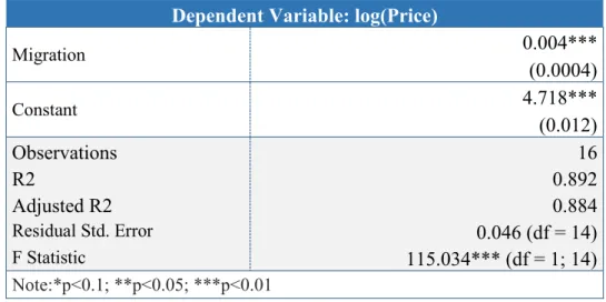
Firstly just with Net-Migration is presented below:

Dependent Variable: log(Price)

Migration 0.004*** (0.0004) Constant 4.718*** (0.012) Observations 16 R2 0.892 Adjusted R2 0.884 Residual Std. Error _{0.046 (df = 14)} F Statistic 115.034*** (df = 1; 14) Note:*p<0.1; **p<0.05; ***p<0.01 Table 1: Univariate model with Net-Migration

Please note that, in this case, opposed to what the author of the OECD paper did, a log-lin model is used not a log-log model. This is because the migration data have negative values and mathematically a logarithm does not admit negative values.

Interpreting the coefficient of the model:

Migration - if Migration is increased by one unit, the housing prices may increase by 0.4% on average.

According to the OECD paper, although the real house prices are positively related to net migration, the impact of this factor may differ depending on how the housing supply behaves regarding the price signals in that country. Anyway, the strength of this effect will always be week. (Andrews 2010).

As foreseen, this model confirms what theory predicts. Actually the effect of migration on the prices is modest, but positive.

(26)

21 This behavior of net migration is relatively easy to understand. Theoretically speaking, if its value increases, there will be more people looking for a house and prices will go up. Of course, the effect that an increase in demand has on the prices is not linear. Firstly, it depends on the size of migration and on its dimension versus the population’s size. If there is a net increase of 10 thousand immigrants in a country where the total population is around 100 million people, its impact on the demand for houses and consequently on the prices will be null. Secondly, as Andrews (2010) defends, if the housing supply can efficiently respond to an increase in the housing demand, the prices will not be affected. Thirdly, it also depends on the purchasing power of the immigrants. If it is significantly higher than the one of the host country, real estate suppliers will adjust the prices over time.

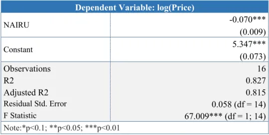
The next model presented is the NAIRU one:

NAIRU -0.070*** (0.009) Constant 5.347*** (0.073) Observations 16 R2 0.827 Adjusted R2 0.815 Residual Std. Error _{0.058 (df = 14)} F Statistic _{67.009*** (df = 1; 14)} Note:*p<0.1; **p<0.05; ***p<0.01 Table 2: Univariate model with NAIRU

NAIRU – if NAIRU is increased by one percentual point, the housing prices may well decrease 7%, on average.

Here again instead of using the log-log model as in the other cases a log-lin model has been used. In this case, the OECD model has been followed.

Comparing with the original paper, here the NAIRU has a more expressive impact than the one observed there (around 8% fall for a 2% increase in unemployment).

(27)

22

The negative impact of NAIRU (non-accelerating inflating rate of unemployment), or Natural Unemployment, on the housing prices is apparently easier to understand. Actually, when unemployment increases unemployed people cannot afford to buy houses and those still holding a job are less confident to borrow. Therefore, the demand decreases and consequently the prices fall as well.

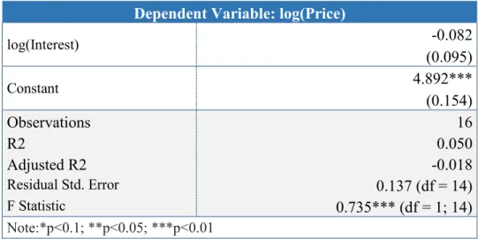
The third model is the one with the Interest Rate:

log(Interest) -0.082 (0.095) Constant 4.892*** (0.154) Observations 16 R2 0.050 Adjusted R2 -0.018 Residual Std. Error 0.137 (df = 14) F Statistic 0.735*** (df = 1; 14) Note:*p<0.1; **p<0.05; ***p<0.01 Table 3: Univariate model with Interest

Interest - if Interest is increased by one percentual point, the housing prices may decrease by 0.082% on average.

Comparing with the original paper, the effect of the interest rate is once again similar to what they obtain.

Interest Rate is, on average, negatively related to house prices (Andrews 2010). Overall results suggest that a decline in real interest rates increases house prices. “This result is consistent with the idea that in countries where there is less competition in the banking sector, financial institutions may pass through less of a given decline in the policy rate to the mortgage rates” (Andrews 2010). As the OECD paper shows in its analysis (page 17, table 1, column 2) when the net margins of interest increase (meaning there is less competition and so a higher interest rate) the housing prices decrease. However, these empirical conclusions may have some

(28)

23 limitations because the net margins may be influenced by other factors as Hawtrey and Liang (2008) conclude.

This relationship between interest rate and housing prices is reasonable. An interest rate increase represents that money gets more expensive for the households needing to borrow when buying a house. Consequently, the rational decision of the borrower when reacting to this increase is to borrow less, decreasing the demand for housing and consequently the prices will go down.

The fourth model is the one with Income:

log(Income) -0.976** (0.398) Constant 14.792*** (4.092) Observations 16 R2 0.300 Adjusted R2 0.250 Residual Std. Error _{0.118 (df = 14)} F Statistic 6.008** (df = 1; 14) Note:*p<0.1; **p<0.05; ***p<0.01 Table 4: Univariate model with Income

Income – if Income is increased by one unit, the housing prices may fall 0.976% on average.

When comparing this result with the one in the original paper, the coefficient is different as well as the impact on prices, which is the opposite. This goes against empirical and theoretical knowledge.

Naturally, it is reasonable to conclude that the higher the households’ disposable income the more propitious they are to consume and invest in real estate.

In theory, reasoning inside the same behavioral framework of setting the loan amount according to a maximum effort ratio, as explained in the beginning of this chapter, the loan will be higher

(29)

24 and so will the demand and probably the price too, (given the interest rate) the higher the disposable income.

However, the econometric model proved the opposite. The fact that just one variable in the model is included is one of the reasons for this weird relationship. Probably having a more exhaustive econometric model, similarly to what the OECD paper where Income is being analyzed along with other variables, the coefficient would be positive (confirming theory). Another reason for this is the period being analyzed. The housing prices had grown so much in the previous decade that at the beginning of the century they had to adjust negatively although the disposable income was still rising.

Yet, it should not be forgotten that the agents involved are humans. This means that even with the average disposable income already increasing, people may be expecting that housing prices will still fall delaying their decisions.

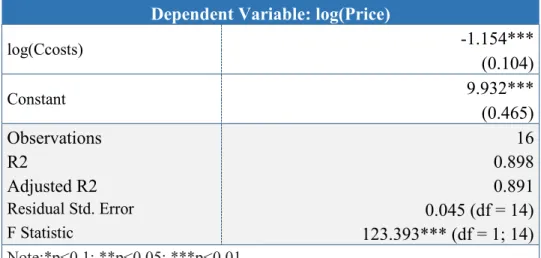
The next model is the one related to Construction Costs.

In the original paper, this variable is incorporated in the variable Z. This variable, as explained above, also includes dwelling stock per capita and rental costs. It is not included in this dissertation for a couple of reasons. Firstly, Construction Costs is the most significant variable in the original regression just as Andrews (2010) defends “real rental costs and the dwelling stock are not significant”. Secondly trustable and complete information for these variables could not be found.

log(Ccosts) -1.154*** (0.104) Constant 9.932*** (0.465) Observations 16 R2 0.898 Adjusted R2 0.891 Residual Std. Error _{0.045 (df = 14)} F Statistic _{123.393*** (df = 1; 14)} Note:*p<0.1; **p<0.05; ***p<0.01 Table 5: Univariate model with Construction Costs

(30)

25 Interpreting the coefficient of the model:

Construction costs – if Construction Costs is increased by one unit, the housing prices may fall 1,154% on average. This means that an increase of 10%, will have an impact of about 11,5% which is a huge impact.

Comparing these values with the ones in the original paper estimating an increase of 0,4% in prices when construction costs increase 1%, a bigger coefficient with the opposite impact on the prices was found.

It makes sense to think that an increase in Construction Costs may lead to an increase in housing prices (it is more expensive to build a house which is reflected on the price). However, exactly the opposite was found. Considering the data plotted in the next graph (both represented as Indexes) the Construction Costs have been increasing since 2000 while the real housing prices had a huge decline.

Similarly to the variable income, this strange relationship may be explained by both the econometric model itself and the period in analysis. One of the causes for this to happen is the fact that only one variable is included in the model, as explained before. Secondly, housing prices fall a lot as a natural negative adjustment to the big increase observed in the decade before 2000. Construction Costs were not enough to create a turnaround in the price tendency

65 75 85 95 105 115 125 135 145 2000 2001 2002 2003 2004 2005 2006 2007 2008 2009 2010 2011 2012 2013 2014 2015

Construction Costs vs Housing Prices

Housing Prices Construction Costs

(31)

26 at the time due to the crisis dimension the country (as well as other worldwide areas) experienced. Maybe it can be assumed the model is not sufficiently specified.

Finally the last model is the one with Inflation:

log(inflation +1) 0.067* (0.036) Constant 4.702*** (0.045) Observations 16 R2 0.200 Adjusted R2 0.142 Residual Std. Error _{0.126 (df = 14)} F Statistic _{3.489* (df = 1; 14)} Note:*p<0.1; **p<0.05; ***p<0.01 Table 6: Univariate model with Inflation

Inflation – if Inflation is increased by one percentual point, the housing prices may increase 0.067% on average.

The result obtained is very similar to the one presented in the original paper – inflation is practically insignificant.

This is explained by the fact that inflation can have opposite effects depending on how the economy reacts to it. As Stevens (1997) defends “on the one hand, since mortgage debt is extended in nominal terms, higher inflation may increase the longer-term attractiveness of housing debt to the extent that it erodes the nominal value of mortgage debt over time. On the other hand, since financial institutions usually impose lending limits based on maximum effort repayment ratios, lower inflation will imply lower nominal interest rates which will increase the maximum amount a financial institution will lend to the household.”

(32)

27

Univ. Models

ß

Price Impact Significance R2

Migration _0.4% Positive Very Significant 0.892

NAIRU _7% Negative Very Significant 0.827

Interest Rate _0.082% Negative Not Significant 0.050

Av. Disp. Income _0.976% Negative Significant 0.300

Const. Costs _1.154% Negative Very Significant 0.898

Inflation _0.067% Positive Slightly Significant 0.200

Table 7: Univariate model resume

After analyzing these models, a general comparison between them can be made especially using R2_{. Although these univariate regressions are too crude to really explain the evolution of} housing prices, which makes the R2 _{comparison unreliable, it will be done in order to obtain the} most significant variables and consequently do the bivariate models. The criteria used was R2 higher than 0,8. The adjusted R2_{is also a good tool when comparing econometric models in} case they have different number of independent variables. As a consequence, it will be used further on at the end of this chapter.

Migration and Construction Costs are the variables with the highest R2_{followed by NAIRU.} Statistically, it is understood as the models that better explain the housing purchase prices. As explained above, the results obtained with Construction Costs are against the expected relationship. It is to be noted that whereas there is a general tendency to the increase in costs over time, especially in this period coinciding with the Portuguese entry the Euro, the housing prices followed an economic crisis reaching its minimum in 2013.

Another good conclusion to come to out of the resume of the models is that in these three models all the variables are very significant statistically. On the other hand, in the three with the lowest value of R2_{, their variables are not such statistically significant.}

3.4.2 Bivariate

As seen in the models above, the ones with a higher R2_{are “Migration”, “NAIRU” and} “Construction Costs”. So, they will be combined in four different models to observe how they explain the prices.

(33)

28 First, a regression including NAIRU and Net-Migration:

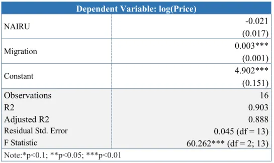
NAIRU -0.021 (0.017) Migration 0.003*** (0.001) Constant 4.902*** (0.151) Observations 16 R2 0.903 Adjusted R2 0.888 Residual Std. Error _{0.045 (df = 13)} F Statistic _{60.262*** (df = 2; 13)} Note:*p<0.1; **p<0.05; ***p<0.01 Table 8: Bivariate model with NAIRU and Migration

Interpreting coefficients:

NAIRU – if NAIRU is increased by one percentual point, the housing prices may fall 2.1% on average.

Migration – if Migration is increased by one unit, the housing prices may increase 0.3% on average.

As expected, the R2_{of both individual regressions is lower than in the bivariate regression and} the coefficients are higher. However, in the bivariate regression, NAIRU lost its significance. Although it maintains a negative coefficient, the fact that it is no longer significant means that in this model Migration can better explain the evolution of housing prices.

(34)

29

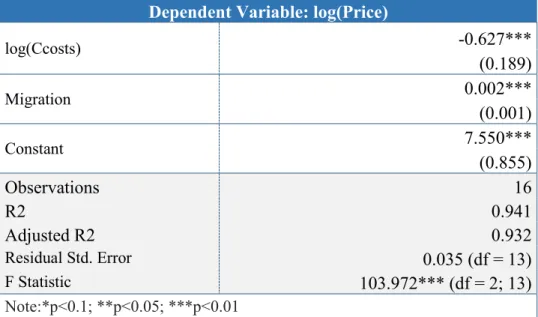
log(Ccosts) -0.627*** (0.189) Migration 0.002*** (0.001) Constant 7.550*** (0.855) Observations 16 R2 0.941 Adjusted R2 0.932 Residual Std. Error _{0.035 (df = 13)} F Statistic _{103.972*** (df = 2; 13)} Note:*p<0.1; **p<0.05; ***p<0.01 Table 9: Bivariate model with Construction Costs and Migration

Construction Costs – if Construction Costs is increased by one unit, the housing prices may fall 0.627% on average.

Migration – if Migration is increased by one unit, the housing prices may increase 0.2% on average

In this case the R2_{is well above 0,9 theoretically meaning that the model explains the price} evolution very well. Comparing with the univariate models, both variables keep very significant. Construction Costs’ coefficient is still negative which, as explained above, is against the theory (and other studies as well including OECD paper) however it can be justified when considering the period in analysis.

(35)

30

log(Ccosts) -0.853*** (0.245) NAIRU -0.021 (0.016) Constant 8.757*** (0.980) Observations 16 R2 0.911 Adjusted R2 0.897 Residual Std. Error _{0.044 (df = 13)} F Statistic _{66.242*** (df = 2; 13)} Note:*p<0.1; **p<0.05; ***p<0.01 Table 10: Bivariate model with NAIRU and Construction Costs

Construction Costs – if Construction Costs is increased by one unit, the housing prices may decrease 0,853% on average.

NAIRU – if NAIRU is increased by one percentual point, the housing prices may decrease 2,1% on average

Following what happened in the previous bivariate regressions, NAIRU lost its econometric significance and Construction Costs keep very significant although with a negative coefficient.

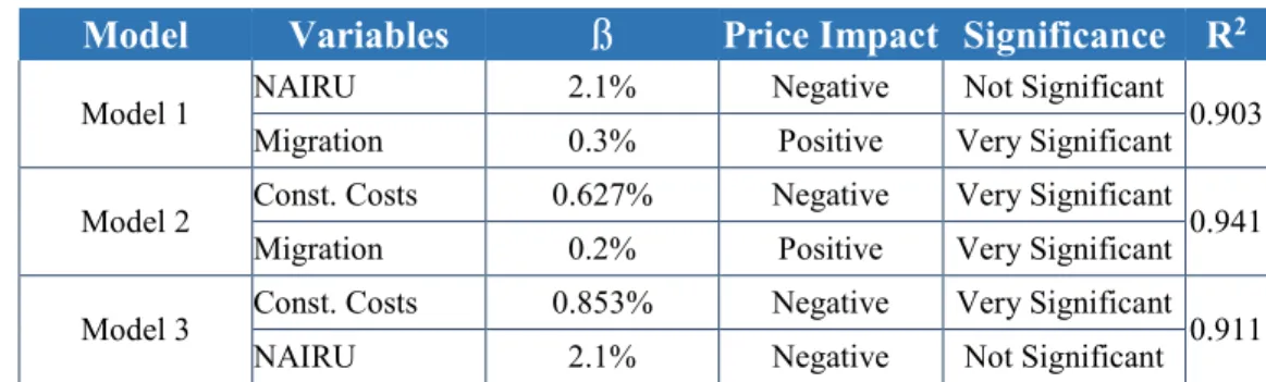
The next table resumes the results of the bivariate regressions.

Model Variables

ß

Price Impact Significance R2

Model 1 NAIRU 2.1% Negative Not Significant 0.903

Migration 0.3% Positive Very Significant

Model 2 Const. Costs 0.627% Negative Very Significant 0.941

Migration 0.2% Positive Very Significant

Model 3 Const. Costs 0.853% Negative Very Significant 0.911

NAIRU 2.1% Negative Not Significant

(36)

31 3.4.3 Multivariate

Now, consider the behavior of the three variables together.

log(Ccosts) -0.631** (0.225) NAIRU 0.001 (0.016) Migration 0.002** (0.001) Constant 7.561*** (0.957) Observations 16 R2 0.941 Adjusted R2 0.926 Residual Std. Error _{0.037 (df = 12)} F Statistic _{63.988*** (df = 3; 12)} Note:*p<0.1; **p<0.05; ***p<0.01

Table 12: Bivariate model with Construction Costs, NAIRU and Migration.

Construction Costs – if Construction Costs is increased by one unit, the housing prices may fall 0,631% on average.

NAIRU – if NAIRU is increased by one percentual point, the housing prices may increase 0,1% on average

Migration – if Migration is increased by one unit, the housing prices may increase 0.2% on average

When observing the R2_{the conclusion is that it is roughly the same as the one of the} regressions just with the dependent variables Migration and Construction Costs. NAIRU is a non-significant variable and its coefficient becomes almost zero. Both Construction Costs, that kept negative, and Migration lost significance comparing with their bivariate regressions.

(37)

32 After the individual analysis of the bivariate regressions, it may be observed that its R2 _is significantly higher than in the univariate regressions as it is expected.

In what regards the adjusted R2_{, the model with the highest value is the one with} Construction Costs and Migration meaning that is the model theoretically better explaining the prices for Portugal taking into consideration the period in analysis.

The final model including the three most significant variables also has a very high adjusted R2_{although lower than the one with only Migration and Construction Costs.}

In conclusion, after analyzing all the models specified, none of them are satisfying once there are only two significant variables and one of them has the opposite sign to the one expected. This is certainly caused by the very strange period of analysis considered.

A good conclusion that can be considered as relevant and trustable is that the demographic influence is the most important. Maybe in future research further variables different from the ones indicated in the OECD paper can be included to capture the behavior in the pre- and post-crisis period.

(38)

33 4. Conclusion

After the theoretical, empirical and econometric analysis made, it was possible to come to conclusions. Limitations of the dissertation must also be taken into consideration as well as possible improvements for future research.

The straight answer to the research question stated in Introduction is that the demographic issues are the most relevant shock affecting housing prices positively. This shock is explained by the fact that an increase in Population, either through immigration or through birth rates, will induce an increase in demand for housing and consequently in prices, especially when the Supply takes too long to adjust (which is characteristic from real estate industry). Regarding the impacts of structural and policy factors they proved to be inconclusive either because they were not significant in the regressions or the regressions showed an impact opposite to what was expected (the reasons for this are linked with limitations explained below).

After running the bivariate regressions and the multivariate regression with the three most significant variables (Migration, Construction Costs and NAIRU), it is believed the model that better explains the housing prices in Portugal, using the adjusted R2_{as the criterium, is the one} having Migration and Construction Costs as independent variables. However, Construction Costs’ impact was the opposite to the expected (the models showed a negative relationship between Construction Costs and Real Housing prices which goes against the expected relationship).

Regarding the question whether Portugal is identical in demographic terms to the “OECD prototype” it was proven that it follows the same path: an increase in total population will lead to an increase in demand for housing and consequently an increase in prices.

Finally answering the question if it is necessary to take some other issues into consideration when analyzing this period (2000 to 2015) in Portugal, the conclusion is that made it within a wider time lag must be analyzed. This wider time horizon is also crucial to dilute the troublesome effects of the recent economic crisis, in order to achieve a more solid analysis. There are also some obvious limitations to this analysis. Firstly, it was impossible to obtain data for all the variables included in the original paper. Even for the variables found useful and trustable information, the oldest data obtained were just from the year 2000 onwards meaning that with this shorter period (16 years instead of 25) and just one country instead of all countries of OECD, the comparison with the original paper using the same econometric model became tricky and so it was necessary to make some adjustments.

(39)

34 The period in analysis was also a huge, and probably the greatest limitation. As explained in the Literature, the period was a very sensible one for Portugal. The big economic crisis was transversal to every sector of the society (Real Estate included) and it is virtually impossible to establish a reasonable and solid econometric relationship between housing–price-evolution and other macroeconomic aspects without taking other factors into consideration.

Regarding the univariate regressions, in spite of the fact that they don’t have too much econometric significance, they were run as a means not only of making the first comparisons with OECD paper (weak comparisons) but also especially of using the R2_{as a criterium to} choose the most significant variables to build and run the econometric regressions with two, or more, independent variables.

On the one hand the fact that from the six variables in analysis just two of them proved significant (Migration and Construction Costs) it does not allow any satisfaction with the results, especially when one of the impacts of these variables – Construction Costs – is against the expected relationship. On the other hand, the good conclusion was to prove that when analyzing a sensible economic period for a certain region or country the approach must be different.

As a possible future research, it is believed that investing more time trying to get information for all the variables included in the OECD econometric model and analyzing a wider time lag (for example from 2000 to 2030) would be interesting. It will allow not only to observe the real behavior of the variables affecting the prices in Portugal but also to make a direct trustworthy comparison with the OECD paper as thought possible when first choosing to develop this topic in this dissertation.

(40)

35 5. Bibliography

Abelson, P., R. Joyeux, G. Milunovich and D. Chung (2005), "Explaining House Prices in Australia: 1970- 2003", Economic Record, Vol:81 S96–S103.

Apergis, N. (2003). “Housing Prices and Macroeconomic Factors: Prospects within the European Monetary Union”, Housing Prices and Macroeconomic Factors Vol.6:63-74.

CaixaBank (2017). “The awakening of the Portuguese real estate market”, 21st of September of 2018 from

http://www.caixabankresearch.com/sites/default/files/documents/im_1712_22_f6_en.pdf.

Capozza, D., P. Hendershott and C. Mack (2004), “An Anatomy of Price Dynamics in Illiquid Markets: Analysis and Evidence from Local Housing Markets," Real Estate

Economics 32(1):1-32.

Catte, P. N. Girouard, R. Price and C. André (2004), "Housing Markets, Wealth and the Business Cycle”, OECD Economics Department Working Papers No. 394, OECD, Paris.

Chanpiwat, N. (2013). "Estimating the impact of immigration on housing prices and housing affordability in New Zealand". 30th of November of 2018 from externalfile:drive8d147e9b3f943081ff65765680f2491745e659cb/root/6.pdf.

Degen, K. and A.M. Fisher (2009), "Immigration and Swiss House Prices”, Centre for Economic Policy Research Discussion Paper 7583.

Fan K. and Peng W. (2003), Real estate indicators in Hong Kong SAR, 124.

Feldstein, M. S. (1992), Comment on James M. Poterba’s paper, tax reform and the housing market in the late 1980s : who knew what, and when did they know it?, in L. Browne and E. S. Rosegren (eds.), Real Estate and Credit Crunch, Federal Reserve Bank of Boston Conference

Series, 36, 252-257.