School retention rates in portuguese municipalities: a comparative analysis

(1)

i an

School retention rates in Portuguese

municipalities

Rita Marques Costa

A comparative analysis

Dissertation presented as a partial requirement for obtaining

the Master’s degree in Statistics and Information

(2)

ii

OVA Information Management School

Instituto Superior de Estatística e Gestão de Informação

Universidade Nova de Lisboa

SCHOOL RETENTION RATES IN PORTUGUESE MUNICIPALITIES:

A COMPARATIVE ANALYSIS

by

Rita Marques Costa

Dissertation presented as a partial requirement for obtaining the Master’s degree in Information Management, with a specialization in Information Analysis and Management

(3)

iii

June 2019

(4)

iv

ACKNOWLEDGMENTS

First of all, thanks to professor Paulo Pinho Gomes. Who was incredibly generous and always

available along the process. Thanks for being demanding, realistic and for always being ready

to listen and answer to my questions. This project would not have moved forward without

his precious guidance. Special thanks also to professor Jorge Mendes for his advice during

the development of this dissertation.

The most important lesson I have learned in the past two years was not to give up. I thank

Helena for never letting me do so and for her unconditional support; my parents, and my

sister for being my greatest inspiration and example of resilience and hard work - I would

not be half of what I am today without them; Ricardo for listening to my very specific

technical questions; my grandparents and Rafa, for keeping my heart warm; Cláudia and

Zara for making this long road so much fun and for teaching me so much.

(5)

v

ABSTRACT

One of the measures used to evaluate the success of an education system is the retention rate. In Portugal, in spite of the progress achieved in the past decades, students’ retention is still a problem. The phenomenon of school failure has been extensively studied throughout the world. Nevertheless, the way it is distributed across the country and the potential reasons that contribute to it being more intense in some areas than in others have not. The idea behind this project is to analyze the retention rates in middle school and in high school in the Portuguese public system, since the beginning of the decade and understand how they are distributed across the territory. The methods used were Principal Components Analysis and cluster analysis.

The data related to potentially explanatory indicators of student failure – such as the average number of students per class, percentage of students in families who benefit from social support and the percentage of teachers with a permanent contract – were analyzed.

The differences between the north and the south of the country are remarkable. Generally, the retention rates are much higher in the south than in the north. We also conclude that municipalities that are closer to each other have similar behaviors regarding their students’ success or unsuccess in terms of retention rates. Nevertheless, there are exceptions to the rule. For example, in Algarve, São Brás de Alportel stands out as a municipality that does particularly well in a context where retention rates are relatively high.

Lastly, in this dissertation, we zoomed in the conurbations of Lisboa and Porto, where almost one in four children was enrolled in 2015/2016. The conclusions are striking: there are schools with some of the lowest retention rates while others, sometimes right across the street, can double the percentage of retained students.

KEYWORDS

(6)

vi

INDEX

1. Introduction ... 1

2. Literature review ... 3

2.1. The concept ... 3

2.2. National and international data ... 3

2.3. The impacts ... 3

2.4. Geographical distribution ... 5

2.5. Priority intervention ... 6

2.6. International examples ... 6

3. Methodology ... 8

3.1. Data description ... 8

3.2. Principal components analysis ... 11

3.3. Cluster analysis ... 11

3.4. Workflow ... 12

4. Results and discussion ... 13

4.1. Principal components ... 14

4.1.1. First principal component (PC1) ... 14

4.1.2. Second principal component (PC2) ... 16

4.1.3. Third principal component (PC3) ... 18

4.1.4. Fourth principal component (PC4) ... 19

4.1.5. Fifth principal component (PC5) ... 21

4.1.6. Sixth principal component (PC6) ... 22

4.1.7. Seventh principal component (PC7) ... 24

4.1.8. Eighth principal component (PC8)... 25

4.1.9. Ninth principal component (PC9) ... 26

4.1.10. Tenth principal component (PC10)... 28

4.2. Cluster analysis ... 29

4.2.1. Cluster one: the not so good and not so bad ... 31

4.2.2. Cluster two: the peak in 12th grade between 2010/2011 and 2011/2012 . 32

4.2.3. Cluster three: the peak in 12th grade in 2012/2013 and 2013/2014 ... 32

4.2.4. Cluster four: bad in 10th and in 12th grade ... 33

4.2.5. Cluster five: the best performing municipalities ... 34

4.2.6. Cluster six: the worst performing municipalities ... 35

(7)

vii

4.2.8. Additional data ... 36

4.2.9. A closer look into each territory ... 37

4.3. Zoom in Lisboa and Porto ... 51

4.3.1. Lisboa in middle school ... 52

4.3.2. Lisboa in high school ... 55

4.3.3. Porto in middle school... 56

4.3.1. Porto in high school ... 59

4.4. TEIP schools ... 61

5. Conclusions ... 65

6. Limitations and recommendations for future works ... 66

7. Bibliography ... 67

8. Appendix ... 69

(8)

viii

LIST OF FIGURES

Figure 1 – Example boxplots for 9th grade 2010/2011 (left) and for 12th grade 2011/2012

(right) ... 8

Figure 2 – Evolution of median retention rates in each school level along the years under

study ... 10

Figure 3 – Workflow ... 12

Figure 4 – Screeplot ... 14

Figure 5 – Principal Component 1 ... 15

Figure 6 – Axis 1 ... 15

Figure 7 – Geographic distribution of the municipalities in PC1 ... 16

Figure 8 – Principal Component 2 ... 16

Figure 9 – Axis 2 ... 17

Figure 10 – Geographic distribution of the municipalities in PC2 ... 17

Figure 11 – Principal Component 3 ... 18

Figure 12 – Axis 3... 18

Figure 13 – Geographic distribution of the municipalities in PC3 ... 19

Figure 14 – Principal Component 4 ... 20

Figure 15 – Axis 4... 20

Figure 16 – Geographic distribution of the municipalities in PC4 ... 20

Figure 17 – Principal Component 5 ... 21

Figure 18 – Axis 5... 21

Figure 19 – Geographic distribution of the municipalities in PC5 ... 22

Figure 20 – Principal Component 6 ... 23

Figure 21 – Axis 6... 23

Figure 22 – Geographic distribution of the municipalities in PC6 ... 23

Figure 23 – Principal Component 7 ... 24

Figure 24 – Axis 7... 24

Figure 25 – Geographic distribution of the municipalities in PC7 ... 25

Figure 26 – Principal Component 8 ... 25

Figure 27 – Axis 8... 26

Figure 28 – Geographic distribution of the municipalities in PC8 ... 26

Figure 29 – Principal Component 9 ... 27

Figure 30 – Axis 9... 27

Figure 31 – Geographic distribution of the municipalities in PC9 ... 27

(9)

ix

Figure 33 – Axis 10... 28

Figure 34 – Geographic distribution of the municipalities in PC10 ... 28

Figure 35 – Clustering methods comparison ... 29

Figure 36 – Distribution of retention rates trimean along the years in each cluster ... 30

Figure 37 – Cluster 1 ... 31

Figure 38 – Cluster 2 ... 32

Figure 39 – Cluster 3 ... 33

Figure 40 – Cluster 4 ... 34

Figure 41 – Cluster 5 ... 34

Figure 42 – Cluster 6 ... 35

Figure 43 – Cluster 7 ... 36

Figure 44 – Boxplots for additional data ... 37

Figure 45 – Alentejo Central ... 39

Figure 46 – Alentejo Litoral ... 39

Figure 47 – Algarve ... 40

Figure 48 – Alto Alentejo ... 41

Figure 49 – Alto Minho ... 41

Figure 50 – Alto Tâmega ... 42

Figure 51 – Área Metropolitana de Lisboa ... 43

Figure 52 – Área Metropolitana do Porto ... 44

Figure 53 – Ave ... 44

Figure 54 – Baixo Alentejo... 45

Figure 55 – Beira Baixa ... 45

Figure 56 – Beiras e Serra da Estrela ... 46

Figure 57 – Cávado ... 46

Figure 58 – Douro ... 47

Figure 59 – Lezíria do Tejo ... 47

Figure 60 – Médio Tejo ... 48

Figure 61 – Oeste ... 48

Figure 62 – Região de Aveiro ... 49

Figure 63 – Região de Coimbra ... 49

Figure 64 – Região de Leiria ... 50

Figure 65 – Tâmega e Sousa ... 50

Figure 66 – Terras de Trás-os-Montes ... 51

Figure 67 – Viseu Dão Lafões ... 51

(10)

x

Figure 69 – Boxplot for retention rates in Lisboa’s middle schools in each cluster and school

level from 7th (left) to 9th (right). ... 53

Figure 70 – The case of Oeiras ... 53

Figure 71 – The case of Olivais and Telheiras ... 54

Figure 72 – Great diferences in the center of Lisboa ... 54

Figure 73 – Retention rates in Lisboa’s high schools ... 55

Figure 74 – Boxplot for retention rates in Lisboa’s high schools in each cluster and school

level from 10th (left) to 12th (right)... 55

Figure 75 – The case of Amadora and the center of Lisboa ... 56

Figure 77 – Boxplot for retention rates in Porto’s middle schools in each cluster and school

level from 7th (left) to 9th (right). ... 57

Figure 76 – Retention rates in Porto’s middle schools ... 57

Figure 78 – The case of Foz do Porto and Covelo ... 58

Figure 79 – The case of Bairro do Cerco ... 58

Figure 80 – Retention rates in Porto’s high schools... 59

Figure 81 – Boxplot for retention rates in Porto’s high schools in each cluster and school level

from 10th (left) to 12th (right). ... 60

(11)

xi

LIST OF TABLES

Table 1 – Impacts of retention on students ... 5

Table 2 – Data description ... 10

Table 3 – Eigenvalues obtained from PCA ... 13

Table 4 – Cluster statistics (part I) ... 29

Table 5 – Cluster statistics (part II) ... 30

Table 7 – Additional data (median rates in 2015/2016) ... 36

Table 8 – Weighted coefficients of variation for the NUTs III ... 38

Table 9 – Evolution of TEIP schools in middle school levels between 2010 and 2016 ... 63

(12)

xii

LIST OF ABBREVIATIONS AND ACRONYMS

DGE Direção-Geral da Educação

EB Escola Básica (middle school)

ES Escola Secundária (high school)

EBS Escola Básica e Secundária (middle and high school)

INE National Statistics Institute

NUT Nomenclature of Territorial Units for Statistics

PCA Principal Components Analysis

PC Principal Component

TEIP Territórios Escolares de Intervenção Prioritária (translates to school territories of priority intervention)

(13)

1

1. INTRODUCTION

To retain a student is to make him or she repeat the school level that was finished in a given year instead of allowing them to move forward. This practice is usually justified as a way to reduce any shortcomings in students' academic progress (Jimerson, 1997 in Ferreira et al., 2015)

Several authors have argued though that this type of practice has significant impacts on the students that are subjected to it. And it is very rare for authors to cite positive consequences for the retained children or adolescents (Ferreira et al., 2015). On the contrary, lower self-esteem, early school leaving, poorer financial and creative capabilities during adulthood and a significant toll in the school and state’s budget are some of the most common impacts enumerated by Ferreira et al. (2015). In general, Portugal shows clear improvements in the effort to reduce the school retention rate. Particularly since the beginning of the century. But it is still one of the European countries where this statistic is higher. For Pereira & Reis (2014) the country is actually an example of a place where making a student repeat one year “is common practice” and it is embedded in the school culture (Sousa, 2017).

In spite of that, grade repetition is not homogeneous throughout the Portuguese territory. There are places where the ratio of retained students is higher than in others. That has to do with students’ socioeconomic conditions and with the specificities of the territories themselves as Justino et al. (2014) and Pereira & Reis (2014) put it. Recognizing that this characteristics can (and have) impact on the schools results, the Portuguese Ministry of Education implemented a program called TEIP – which is an acronym for educative territories of priority intervention – that is aimed at schools located in “economically and socially disadvantaged areas, marked by poverty and social exclusion, where violence, indiscipline, abandonment, and school failure are most evident” (DGE, 2016). Taking all this into consideration, the goal of this project is to understand how the school retention rates are distributed in the country by analyzing data for each municipality since 2010 for six different school levels – 7th, 8th, 9th, 10th, 11th, and 12th. The Portuguese school system (which is of mandatory enrolment until the age of 18 since 2009) is divided into three main groups: primary school, middle school (split into the second and third cycle) and high school. The grades under analysis correspond to what is called in Portugal the third cycle of middle school and high school. By using the different grades and multiple school years the aim is to capture the diversity in the growth trends of the indicator, such as Justino & Santos (2017) did when analyzing other measures of unsuccess. Also, these are the school levels where retention is higher. In the years chosen, the Portuguese population has also gone through severe challenges because of the financial, economic and social crisis so it will be interesting to understand if these reflect on the retention rates.

Do neighbor territories have similar retention rates? Is the phenomenon bigger in the countryside or in coastline areas? In the places where school retention strongly differs from the average do the indicators regarding social support, the average number of students per class or the ratio of professors with a permanent contract also stand out? These are some of the questions that we intend to answer.

(14)

2 Regarding data analysis, the first step was to run a PCA of the school retention rates in each municipality and then cluster the individuals based on those results. After that, the territories that stand out were analyzed further in order to understand what makes them have a particularly bad (or good) performance in this indicator. An analysis focused solely on retention rate in the conurbations of Lisboa and Porto was also applied.

This type of analysis focused solely on school retention rate in public schools of each municipality was never done. One thing that is clear is that not every data related to school failure is in the hands of the local governments. Nevertheless, at a time when the decentralization of education is being discussed, and there will be more local power to manage this field it is relevant for policymakers to have this specific information.

(15)

3

2. LITERATURE REVIEW

2.1. T

HE CONCEPT

The school retention rate measures the proportion of students in a given year who do not advance to the next one. It is a concept that corresponds to the situation of a student staying at the same level of education for an additional year instead of advancing to the above level at the same time as his or her peers (Brophy, 2006) as quoted in (Ferreira, Félix, & Perdigão, 2015). The goal is to reduce any shortcomings in students' academic progress (Jimerson, 1997) in (Ferreira et al., 2015), but some authors also state that it is a "measure that sanctions and which, to a greater or lesser extent and depending on the school level and the age at which the students meet, can diminish their self-esteem, revolt them, disinterested them in the school and demote them from commitment to learning" (Rebelo, 1992; 1999) in (Ferreira et al., 2015).

INE (2018) calculates this indicator based on the number of students in one school level who stay in that same level because they are unsuccessful or because they are voluntarily trying to get better grades, divided by the total number of the students in that school level.

2.2. N

ATIONAL AND INTERNATIONAL DATA

In Portugal, the retention rate has been decreasing. At the beginning of the 2000s, 18.2% of public and private school students in Portugal had been retained. In 2016 this figure fell to 10% (Direcção-Geral de Estatísticas da Educação e da Ciência, 2018). In primary education, in 2001, 12.7% of students were retained. In 2017 they were 5.5%. In high school, the reduction was even greater, from a rate of 39.4% at the beginning of the millennium to 15.1% in 2017. (DGEEC, 2018)

The decrease was even higher in the rate of early school leaving than in the retention rate. "There is a greater emphasis on promoting learning success, which leads to a higher retention rate and a lower number of early school leavers" (Sousa, 2017).

In spite of the positive progress, the latest data from the International Program for Student Assessment (PISA, 2015), indicates that Portugal is the third country in the OECD where more 15-year-olds report having been retained at least once. Ahead of Portugal, there is only Belgium and Spain. According to PISA (2015) data, "in general, in OECD countries, students with socioeconomic, immigrant and youth deficiencies are more likely to have repeated one year".

In Portugal, the law makes school mandatory until children are 18 years old since 2009 (Law 85/2009). The students enrolling in 7th grade and levels below in 2009 were the ones that started to be covered by the new rules. So, the first ones only reached 12th grade in 2014/2015. That resulted in an increase in the number of students enrolled in high school (Viana, 2017). Judging by the global drop in retention rates previously presented, this modification did not have a negative impact on school unsuccess.

2.3. T

HE IMPACTS

The impacts of the retention phenomenon in children and adolescents occur at various levels (Ferreira et al., 2015) and ultimately costs money. Researchers at the Portuguese research project called Aqeduto adapted estimates from the Education Endowment Foundation to conclude that

(16)

4 retaining a student costs 6000 euros per year (Aqeduto, n.d.). Among the measures used to fight school unsuccess, researchers concluded that this is the most expensive and also the most inefficient approach – the student finishes the repeated level with less knowledge than when started.

The table below adapted from Ferreira et al. (2015) shows some of these effects.

Impacts Description

Self-esteem • Retaining students do not contribute to better learning or

to achieving pedagogical goals in subsequent years but increases the probability of dropout and decreases self-esteem (Jimerson, 2001) apud (Ferreira et al., 2015). • Retention leads to decreased self-esteem, impairs the

socialization process and contributes to the alienation of the school according to Brophy (2006) and Xia Kirby (2009) apud (Ferreira et al., 2015).

• "It is worth mentioning that early school retention may lead to a decrease in the student's self-esteem and lead either to the weakening of school ties or to a tendency to interact with deviant peers." (Simões et al., 2008: 148) apud (Ferreira et al., 2015).

Early school leaving • Retention is a significant predictor of school dropout by

students in the secondary level of education according to EACEA/Eurydice (2014) apud (Ferreira et al., 2015).

• Increases the probability of eventual abandonment according to Brophy (2006) and Xia Kirby (2009) apud (Ferreira et al., 2015).

Financial capacity and creativity

• "These students have much lower expectations of training than students who never repeat, this is a cost that will be perpetuated for entire lives, both financially, as well as the creative and productive capacity of these young people, and consequent contribution in human and financial capital to the whole system. "(Flores et al., 2013) apud (Ferreira et al., 2015).

School and state budget and finances

• Brophy (2006) and Xia Kirby (2009) apud (Ferreira et al., 2015) point out that it creates budgetary and patrimonial problems for schools and educational systems.

• The retention costs for Education budgets are substantial. In short, retention is inefficient, costly, having implications for efficiency and equity, say Field et al. (2007); OECD (2012); OECD (2013) apud (Ferreira et al., 2015).

Adjust students’ capacities

• “The stated goal of repeating the failed grade level is to remediate academic failure or social immaturity. Many educators who support the practice of retention believe that it is an effective solution to school failure or maladjustment” (Goodlad & Anderson, 1963) apud (Jimmerson, 1997) apud (Ferreira et al., 2015).

• Nevertheless, Shepard and Smith (1990) concluded that “although grade retention is widely practiced, it does not help children to ‘catch up.’ Retained children may appear to do better in the short term, but they are at much

(17)

5 greater risk for future failure than their equally achieving, nonretained peers” (Jimmerson, 2001) apud (Ferreira et al., 2015).

Table 1 – Impacts of retention on students

2.4. G

EOGRAPHICAL DISTRIBUTION

The distribution of this phenomenon is not the same for each level of education, school or municipality. As Brophy (2006) explains: "The poor performance patterns of those repeating the year tend to be associated with indicators of poverty both at school and in the family. Schools in poor areas (especially remote rural areas) often have limitations: short school years, frequent teacher absenteeism, limited supplies, low-skilled teachers, large classes, multi-age classes, or double-shift classes. Within any school, students from poorer families are at greater risk of repetition because their origins leave them less prepared to succeed and are likely to miss more school days. "

According to Justino et al. (2014) “the contrast between urban and rural areas, the north and south of the country, the interior at risk of desertification and the coastline that concentrates a high proportion of the population, is so striking that it is difficult to speak of territorial cohesion". The problem is also more evident in more isolated schools and in classes with many students (Wong, 2018).

In a 2016 study, DGEEC (2016a) also assesses the impact of the socioeconomic context of school retention. It concludes that children of lower socioeconomic levels may suffer more from retention, but other factors must be taken into account. "The influence of local factors such as the dynamism of schools and their teachers, the degree of importance placed in teaching children and school work in the region's culture, may perhaps overlap locally with the effect of socioeconomic status, so that pupils from regions with low socioeconomic levels may nevertheless have school performance levels in the second cycle, which are clearly higher than the national average. For the third cycle, the conclusions are similar. (DGEEC, 2016b)

In studies that focus on the role of education in specific municipal strategies, the local authorities are already looking at how their municipality is positioned in relation to the neighbors of the same region.

For example, in Lousã, "in the school year 2012/2013, the value of 11.3% [retention] was well above the average of the region, with only the innermost and mountainous municipalities having higher retention. The completion/transition rate in secondary education, with 76.7%, is well below the average for the region and the continent" (Cordeiro & Manuel, 2017).

On the other hand, in Alvito, Alentejo, "in terms of retention and dropout rates in primary and secondary education, the trend registered is decreasing, being close to those registered in the Lower Alentejo "(Saúde, Lopes, & Machado, 2018).

In a study at the municipal level focused on gathering the factors – social and organizational – that explain success or unsuccess, Justino & Santos (2017) found out that, the percentage of mothers with a university degree is the “strongest predictor of results”. Aspects such as the country of origin of the students (because of language barriers) and the socioeconomic deficiencies also contribute to explain the phenomenon.

(18)

6 Understanding how these inequalities are distributed can be useful, especially at a time when decentralization of education is being debated. In this field, there are several views on whether education should be the responsibility of municipalities. There are teachers who "do not agree with the transfer of competences to municipalities because they fear that the management of teaching staff will pass to the chambers, causing the loss of autonomy of the school and that the national dimension of teaching, can generate conflicts between school and local authority, which adds to the risk of politicization of educational action "(Carvalho, 2012). However, the councils defend the idea that the transfer of this power to the municipal level can bring benefits and bring education management closer to local politics (Carvalho, 2012).

In the academic year 2019/2020, the management of 43.626 employees and 996 schools will become the responsibility of local authorities. This decentralization will cost 797 million euros (Francisco, 2018).

2.5. P

RIORITY INTERVENTION

The Ministry of Education recognizes that there are differences between territories and that there are schools in “economically and socially disadvantaged areas, marked by poverty and social exclusion, where violence, indiscipline, abandonment, and school failure are most evident” (DGE, 2016). Some of those schools are part of a program called TEIP – which is an acronym for educative territories of priority intervention – and receive financial support to enhance their organizational practices and also their teaching and learning techniques. In 2016 there were 137 schools (or school groups) in this network. The program exists since 2007.

In an evaluation of the first years of the program, the Ministry of Education mentions that between 2007 and 2010, the TEIP schools managed to reduce early school leaving and school absence.

Regarding the violence index at school, “generally, between 2006/2007 and 2009/2010 there was an increase in the number of indiscipline cases registered and a reduction in the gravity level of those cases” (ME, 2010). But this “should not be associated with a deterioration of the school climate, as it reflects an improvement in the capacity to register and respond to these situations” (ME, 2010). There is no reference to retention in this report.

In 2011, though, a group of researchers (Abrantes, Mauritti, & Roldão, 2011) set to evaluate the school and social impacts in seven TEIP schools. On it, one of the school directors notes that “the students' retention rate has improved, but that can only be partially attributed to the fact that it is a TEIP, something relatively new at the time”.

In a later stage of the analysis, we will be looking specifically into this schools performance regarding retention rates. Namely, the ones located in Lisboa and Porto and its bordering municipalities. For that reason, it is important to bear in mind that there are eight TEIP schools in Amadora, 14 in Lisboa, four in Loures and two in Oeiras – for Lisboa – and four in Gondomar, one in Maia, three in Matosinhos, three in Vila Nova de Gaia and eight in Porto.

2.6. I

NTERNATIONAL EXAMPLES

In the USA, Warren (2005) analyzed the high-school completion rates at the state level (though this is not the same as retention, it can be seen as an opposing measure). What the author concluded was

(19)

7 that “since the mid-1970s the national rate at which incoming 9th graders have completed high school has fallen slowly but steadily; this is also true in 41 states. In 2002, about three in every four students who might have completed high school actually did so; in some states, this figure is substantially lower”.

In New Zealand, Pool et al. (2005) went through the differences in school retention in several regions of New Zealand between 1986 and 2001. Only to conclude that they exist. Mainly because of the pre-existing differences between regions and how they historically favor education, and also because of the level of regional development.

(20)

8

3. METHODOLOGY

3.1. D

ATA DESCRIPTION

The data analyzed refers to the retention rates from 2010/2011 to 2015/2016 for the 3rd cycle of "Ensino básico" or middle school - children from 12 to 14 years old - and "Ensino secundário" or high school - 15 to 18 years old - in public schools in mainland Portugal. In total, 231 municipalities are considered - there are cases where there are no secondary schools and, therefore, the municipality in question is eliminated from the analysis - and 36 variables (the school levels in each year).

Since the existing data for retention in each municipality does not disaggregate this rate for public and private schools, it was calculated based on the retention rate in each public school averaged by the weight given by the number of students in each school year under analysis, that is, 7th, 8th, 9th, 10th, 11th and 12th grade. When calculating all the descriptive statistics and PCA, the data regarding each municipality was weighted by the number of students enrolled in each municipality in 2015/2016.

The boxplots show there are outliers in every variable. Both for middle school and high school levels. Some of the biggest variations happen in 7th and 9th grade, for middle school, and 12th grade, for high school (figure 1).

The preliminary analysis of the data allowed to conclude that there are 19 severe outliers, that is the values that are three times above (the third quartile) or below (the first quartile) the interquartile range.

The data used shows significant differences among municipalities. For example, Amadora has, on average, the biggest retention rate (26.9%). It is followed by Sines, Loures, Odivelas, and Mogadouro. On the other end of the scale, there is Mortágua, Caminha, Sever do Vouga and Monção, all below 10%.

There are also differences in the grades and years analyzed. The highest retention rates happen consecutively in 12th grade. The worst value registered is from 2010/2011 and regards Almodôvar’s retention rate for the 12th grade: 71%. The standard deviation is also slightly wider in 12th grade (as shown in table 2). In high school, the lowest retention values are registered in the 11th grade, which is an intermediate level.

Figure 1 – Example boxplots for 9th grade 2010/2011 (left) and for 12th grade 2011/2012 (right)

(21)

9 Regarding the third cycle, the highest retention happens, on average, on 7th grade. And the lowest values happen in 8th grade. This phenomenon where the intermediate levels have a lower rate of unsuccess than the end of the cycle is not unknown. Conselho Nacional de Educação (2018) released a report where they point out “a significant increase [in the retention rate] in the first year of each study cycle, compared to the last year of schooling in the previous cycle”.

Min Max Mean Median Standard deviation Variance 7th grade (2010/2011) 0.0 40.9 15.6 15.2 5.2 26.9 7th grade (2011/2012) 0.0 33.6 17.5 17.2 5.6 30.9 7th grade (2012/2013) 0.0 36.8 16.9 17.0 5.3 28.0 7th grade (2013/2014) 0.0 42.3 17.6 17.8 5.7 32.7 7th grade (2014/2015) 1.4 34.8 16.0 16.1 5.3 27.7 7th grade (2015/2016) 0.0 30.7 13.3 13.3 4.9 24.2 8th grade (2010/2011) 0.0 28.0 10.5 10.3 4.0 15.8 8th grade (2011/2012) 0.0 29.5 12.9 12.4 4.4 19.5 8th grade (2012/2013) 0.0 30.1 14.4 13.9 4.4 19.1 8th grade (2013/2014) 0.0 33.3 13.8 14.1 4.3 18.8 8th grade (2014/2015) 0.0 32.5 10.6 10.2 4.0 16.4 8th grade (2015/2016) 0.0 25.0 8.4 8.6 3.4 11.8 9th grade (2010/2011) 0.0 37.5 14.3 14.2 4.5 20.3 9th grade (2011/2012) 1.4 40.0 17.6 17.1 5.2 26.6 9th grade (2012/2013) 2.0 41.0 18.6 19.5 4.9 23.5 9th grade (2013/2014) 2.2 34.4 16.1 16.8 4.4 19.1 9th grade (2014/2015) 0.0 25.5 11.3 11.0 3.8 14.4 9th grade (2015/2016) 0.0 23.7 9.5 9.8 3.5 12.3 10th grade (2010/2011) 2.0 43.1 18.5 18.3 5.7 32.2 10th grade (2011/2012) 1.4 42.4 18.0 18.2 6.0 36.6 10th grade (2012/2013) 0.0 47.8 17.4 18.7 5.7 32.4

(22)

10 10th grade (2013/2014) 0.0 35.5 17.5 18.0 5.4 29.0 10th grade (2014/2015) 0.0 35.7 15.9 15.7 5.0 25.5 10th grade (2015/2016) 0.0 33.0 17.7 18.2 5.6 31.4 11th grade (2010/2011) 0.0 38.1 14.0 13.7 4.8 22.7 11th grade (2011/2012) 2.3 33.3 15.3 15.2 4.9 23.8 11th grade (2012/2013) 0.0 29.2 15.4 15.7 4.8 23.3 11th grade (2013/2014) 0.0 32.0 13.6 13.4 4.6 20.9 11th grade (2014/2015) 0.0 26.7 11.5 11.1 4.2 17.7 11th grade (2015/2016) 0.0 23.8 9.0 8.9 3.7 13.5 12th grade (2010/2011) 6.7 71.4 38.9 38.6 6.8 46.4 12th grade (2011/2012) 2.8 60.0 37.2 37.1 6.4 40.4 12th grade (2012/2013) 15.0 67.4 38.1 38.5 7.1 51.1 12th grade (2013/2014) 8.3 65.4 37.4 38.4 7.4 54.2 12th grade (2014/2015) 0.0 62.2 32.3 33.8 7.1 50.7 12th grade (2015/2016) 4.9 54.1 32.3 31.6 7.1 50.2 Table 2 – Data description

The graphs in figure 2 show an interesting phenomenon, particularly in middle school. The retention rates reach a peak between 2012/2013 and 2013/2014 and tend to decrease, reaching lower values than at the beginning of the decade. In high school that is more obvious in 11th and 12th grade. In 10th grade, though that does happen. The percentage of retained students at that level is more or less stable throughout the years.

Figure 2 – Evolution of median retention rates in each school level along the years under study

(23)

11

3.2. P

RINCIPAL COMPONENTS ANALYSIS

For the analysis of retention data, a PCA methodology was used. According to Jolliffe (2002) “the central idea of principal components analysis is to reduce the dimensionality of a data set consisting of a large number of interrelated variables while retaining as much as possible of the variation present in the data set. This is achieved by transforming to a new set of variables, the principal components (PCs), which are uncorrelated, and which are ordered so that the first few retain most of the variation present in all the original variables”. This means that the dimensionality of the retention rates for every grade in each school year will be reduced. Producing a much smaller number of variables.

The variables analyzed are all on the same scale so the covariances matrix was chosen over the correlation matrix to perform the PCA. Also, by keeping the covariance matrix we preserve the differences in variance in the different school years and levels. The covariance matrix shows that the school levels from the same cycle – that is 7th, 8th, 9th, and 10th, 11th 12th – are closer to each other and have bigger covariance when between groups. Even though the matrix of covariances was the one used, we also looked at the correlations. The highest values, around 0.75, happen between the retention rates on 7th grade in several school years. And it is bigger if they are closer in time to each other. This is a sign of the evolution in the indicator, that has reached a peak somewhere between 2012 and 2014 and has been decreasing since then.

As said before, the variables used were weighted by the total number of enrolled students in 2015/2016. The software used to perform the PCA was R. In some instances, SAS Enterprise Guide and Excel were also used. The full results can be seen in the annexed tables.

3.3. C

LUSTER ANALYSIS

The PCA output was then used in the cluster analysis, a method that groups data objects based on the data that describes these objects and their relationships (Tan et al., 2018). With a goal in mind: that the objects within the group are similar to one another and different from the objects in other groups. The greater the similarity (or homogeneity) within a group and the greater the difference between groups, the better or more distinct the clustering, add Tan et al. (2018).

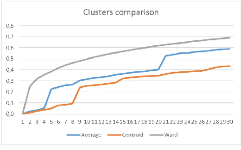
Also, according to Jollife (2002), “there are two main ways in which PCs are employed within cluster analysis: to construct distance measures or to provide a graphical representation of the data; the latter is often called ordination or scaling and is useful in detecting or verifying a cluster structure”. First of all, three different methods of hierarchical clustering were applied in order to evaluate the number of clusters to use in the non-hierarchical k-means. In this stage, the individuals that were considered as severe outliers (and were not included in the PCA) were added to the clustering procedure as supplementary individuals.

The Average method is described as a process that uses the average distance from members of one cluster to members of another cluster as the measure of inter-group distance (Everitt & Skrondal, 2010). In the Single linkage method, the distance between two clusters is deﬁned as the least distance between a pair of individuals, one member of the pair being in each group (Everitt & Skrondal, 2010). The Ward’s method is an agglomerative hierarchical clustering method in which a

(24)

12 sum-of-squares criterion is used to decide on which individuals or which clusters should be fused at each stage in the procedure (Everitt & Skrondal, 2010).

Afterward, the data was clustered with a k-means method. This is a non-hierarchical approach to clustering. Some of the authors behind its introduction were Macqueen (1967) and Diday (1973). Macqueen described it as a process “of partitioning an N-dimensional population into k sets on the basis of a sample”. As for Diday he named the process “dynamic clusters method” (DCM) and explained that “the DCM can be classified among those clustering procedures that have been called ‘iterative relocation procedures’ by some authors and ‘K-means’ and ‘cluster centers’ by others. These various methods start from K points that are drawn either at random or among the population. These K points are chosen as initial centers; all the points are then allocated to the nearest centers”.

3.4. W

ORKFLOW

The workflow diagram can be seen below. The analysis begins with the raw data on retention rates, on which a Principal Components Analysis is performed. Afterward, the data is clustered using both hierarchical and non-hierarchical methods.

(25)

13

4. RESULTS AND DISCUSSION

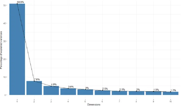
Given that the idea with PCA was to reduce dimensionality to have a clearer picture of how the retention rates evolved, the number of principal components that were taken further into the analysis had to be selected. There is no hard rule on how to make this decision. And there was some iteration throughout the development of this dissertation.

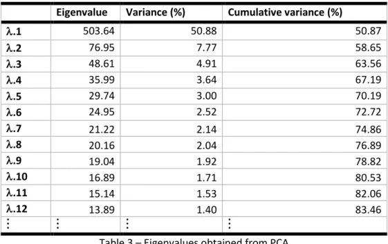
After taking into consideration the scree plot of the eigenvalues and by analyzing the variance retained by each of them, the first decision was to keep the first six principal components. This decision was supported by analyzing the mean of the eigenvalues – 27.5 – which shows that all but the sixth eigenvalue are above that threshold. Together they represent 73% of the inertia associated with the data.

But by going further in the analysis and interpretation of the PCA outputs, it became evident that there were a reasonable number of individuals (93 had a CTR sum in the six dimensions below 50%) that were not well explained by this first six dimensions.

The decision was to go back, and retain the first 10 dimensions of the PCA that together explain 81% of the inertia. In this new scenario, only 36 municipalities are not explained well enough (the inertia of these 36 municipalities is less than 50%).

Eigenvalue Variance (%) Cumulative variance (%)

.1 503.64 50.88 50.87 .2 76.95 7.77 58.65 .3 48.61 4.91 63.56 .4 35.99 3.64 67.19 .5 29.74 3.00 70.19 .6 24.95 2.52 72.72 .7 21.22 2.14 74.86 .8 20.16 2.04 76.89 .9 19.04 1.92 78.82 .10 16.89 1.71 80.53 .11 15.14 1.53 82.06 .12 13.89 1.40 83.46 . . . . . . . . . . . .

Table 3 – Eigenvalues obtained from PCA

(26)

14 The full PCA results can be seen in tables 2 and 3 (annex). The variables with a CTA bigger than 1/36 were taken into consideration for the analysis. As for the individuals, as previously said, there are 36 whose CTR sum in axis 1 to 10 is lower than 50%. Regarding all others: 83 have a CTR sum between 50% and 70%; for 67 the sum is between 70% and 90%; and 26 have a CTR sum along axis 1 to 10 that is greater than 90%.

4.1. P

RINCIPAL COMPONENTS

4.1.1. First principal component (PC1)

The first principal axis explains the relative dimension of retention rates in the universe of public schools in the Portuguese mainland in the school levels targeted in this study and along six years (2010 to 2016). Concretely, the first axis opposes 95 municipalities where the retention rates were clearly lower or much lower than the mean global value of school retention rate to other 49 municipalities where that rate was higher or much higher.

The linear coefficient of correlation between the variables under study and the first principal component is always positive (size effect) and varies between 0.646 and 0.811.

The municipalities that are positioned in the positive side of the first axis are those who present a retention rate that is higher than the mean global value for the years under analysis. The ones on the negative side are those with the values that are lower than the global mean.

The first principal component represents 50.9% of the inertia associated with the data and explains at least 40% of the variance of all the variables under study. The 144 municipalities explain 98% of the inertia associated with the first axis.

All the school years in the 12th grade, 10th grade in 2011/2012 and 7th grade in 2011/2012 are the ones that contribute the most to explain the variance associated with the first axis (this is also

(27)

15

Other municipalities with a relatively high retention rate

Norte

:

Mogadouro; Porto; Matosinhos; Miranda do Douro; Montalegre; Valpaços; Paredes; Torre de Moncorvo; Macedo de Cavaleiros; Alfândega da Fé; Castelo de Paiva; Resende.

Centro: Cadaval; Tábua; Óbidos; Lousã; Anadia; Figueira de Castelo Rodrigo.

Área Metropolitana de Lisboa: Amadora; Odivelas; Loures; Lisboa; Almada; Sintra; Seixal; Moita; Barreiro; Setúbal; Vila Franca de Xira; Sesimbra; Cascais; Alcochete.

Alentejo: Sines; Reguengos de Monsaraz; Benavente; Cartaxo; Odemira; Serpa; Grândola; Vila Viçosa; Beja.

Algarve: Loulé; Albufeira; Vila Real de Santo António; Lagos; Olhão; Portimão; Lagoa; Silves.

Other municipalities with a relatively low retention rate

Norte

:

Vila Nova de Famalicão; Oliveira de Azeméis; Vila Real; Esposende; Amarante; Marco de Canaveses; Guimarães; Caminha; Paredes de Coura; Monção; Espinho; Chaves; Moimenta da Beira; Póvoa de Varzim; Arcos de Valdevez; Santa Maria da Feira; Arouca; Vale de Cambra; Fafe; Penafiel; Vila Nova de Cerveira; Murça; Braga; Carrazeda de Ansiães; Lamego; Vizela; Mesão Frio; Bragança; Cinfães; Melgaço; Amares; Celorico de Basto; Valença; Vila do Conde; Maia; Vila Pouca de Aguiar; Ribeira de Pena.

Centro

:

Figueira da Foz; Covilhã; Coimbra; Viseu; Mortágua; Fundão; Leiria; Marinha Grande; Aveiro; Porto de Mós; Guarda; Entroncamento; Soure; Ovar; Ansião; Cantanhede; Nelas; Castro Daire; Condeixa-a-Nova; Tomar; São Pedro do Sul; Mira; Ourém; Proença-a-Nova; Batalha; Pombal; Oliveira de Frades; Santa Comba Dão; Sobral de Monte Agraço; Oleiros; Trancoso; Torres Vedras; Sátão; Alcanena; Estarreja; Águeda; Vagos; Penacova; Castelo Branco; Penalva do Castelo; Tondela; Mealhada; Sabugal.

Área Metropolitana de Lisboa

:

Oeiras.

Alentejo: Évora; Santarém; Estremoz; Ponte de Sor; Viana do Alentejo; Coruche; Moura.

Algarve: São Brás de Alportel.

confirmed by the correlation matrix between variables and principal components). As previously seen, these are the variables that have a higher variance and a higher mean.

The individuals that are better represented in PC1 are Amadora, Loures, Odivelas, and Lisboa (all in the Lisboa district), to name a few. They all have high retention rates in the school levels that are best represented in this axis. On the other hand, municipalities such as Sever do Vouga, Ponte de Lima, São João da Madeira or Viana do Castelo have lower retention rates in those school years. This first dimension is very important in picturing the biggest and broadest differences between municipalities.

Figure 5 – Principal Component 1

(28)

16

Other relevant individuals to interpret this axis Norte: Paredes; Vila Nova de Gaia; Vale de Cambra; Felgueiras; Macedo de Cavaleiros; Vizela; Valpaços.

Centro: Sobral de Monte Agraço; Tondela; Oliveira de Frades; Figueira de Castelo Rodrigo; Peniche; Alcanena; Penacova; Castelo Branco; Mira; Entroncamento.

Área Metropolitana de Lisboa: Vila Franca de Xira.

Alentejo: Serpa; Moura; Grândola; Benavente; Montemor-o-Novo; Beja.

Algarve: São Brás de Alportel; Vila Real de Santo António; Silves.

Other relevant individuals to interpret this axis

Norte: Resende; Bragança; Lamego; Vila Verde; Tarouca; Mogadouro; Terras de Bouro; Melgaço; Maia; Gondomar; Murça; Alfândega da Fé; Valença; Cinfães; Ribeira de Pena.

Centro: Sátão; Sabugal; Trancoso; Mortágua; Almeida; Gouveia.

Área Metropolitana de Lisboa: Sesimbra; Palmela; Alcochete.

Alentejo: Vila Viçosa; Odemira; Almeirim; Cartaxo.

Algarve: Lagoa.

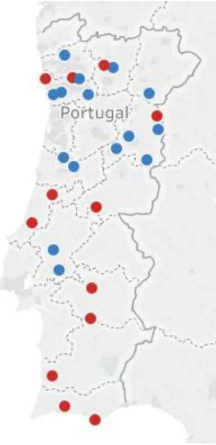
It should be kept in mind that there is already a geographical pattern coming up in the distribution of municipalities in this dimension.

The ones colored in blue in figure 7 are those on the positive half of the axis (and also, globally, the worst performing ones) are mostly in the south of Portugal.

The ones colored in red are the ones that do better. Those are spread in the North, mostly in the municipalities in the coastline.

4.1.2. Second principal component (PC2)

PC2 represents 7.8% of the inertia associated with the data. In PC2 there is an opposition between the variables related to 7th and 12th grade. It is reasonable, then, to assume that this dimension represents the contrast of retention rates in the extreme school levels. From the first grade under analysis to the last one.

Figure 7 – Geographic distribution of the municipalities in PC1

(29)

17 The second axis opposes 33 municipalities where the retention in 12th grade are much higher than those in 7th grade and other 33 where the retention rates for 7th grade is greater than in 12th grade or, in certain cases, both values are very close to each other. These municipalities explain 68.9% of the inertia associated with this axis.

Regarding the municipalities that are better explained by this axis, we confirm (much like in the first dimension) one of the assumptions made in the beginning: there is, in fact, a similar behavior between municipalities that are geographically closer to each other. That is the case, for example, with Cascais and Oeiras, both in the Lisboa district. These municipalities (Águeda, Braga and some others as well) are the ones that perform relatively well in 7th grade, but the retention rate tends to get worse in 12th grade.

Batalha and Caldas da Rainha, both in Leiria, and Lourinhã, located in Lisboa (although these three municipalities are not all part of the same district they are geographically close to each other) show some similarities that are the opposite of the ones previously described. They have, in certain school years, higher retention rates in 7th grade and lower in 12th. Although it must be noted that it is not common that retention rates in 7th grade are higher than those in 12th. In the municipalities that are positioned in the positive side (blue) of this axis, the retention rates in 7th grade tend to be much closer to those obtained in 12th grade than in the municipalities on the other half.

In spite of the proximity between the municipalities that stand out in this dimension, there is no clear geographic pattern associated with the distribution of these schools. But is a higher concentration of municipalities in red (negative side of the axis) in the interior north and Lisboa.

What we observe in this axis, though, is a pattern that needs to be understood. Why do schools have the worst retention rates in 7th grade and get better in 12th? Are the students that retain the most led to pursue professional courses? Because if that is what happens they “disappear” from these statistics (in high school, we are only looking onto the standard choice courses, called “cursos científico-humanísticos” in Portugal).

Figure 9 – Axis 2

(30)

18

Other relevant individuals to interpret this axis:

Norte: Matosinhos; Terras de Bouro; Macedo de Cavaleiros; Montalegre; Braga; Porto; Amares.

Centro: Alenquer; Castelo Branco; Arganil; Oleiros; Estarreja; Águeda; Oliveira do Hospital; Nelas; Sobral de Monte Agraço; Seia.

Área Metropolitana de Lisboa: Vila Franca de Xira.

Alentejo: Beja; Odemira.

Algarve: Portimão; Silves.

Norte: Vieira do Minho; Mesão Frio; Fafe; Felgueiras; Cinfães; Amarante; Arcos de Valdevez; Gondomar; Valpaços; Tarouca; Valongo; Paredes; Carrazeda de Ansiães; Marco de Canaveses; Resende.

Centro: Penalva do Castelo; Gouveia; Almeida;

Marinha Grande; Castro Daire; Lourinhã; Santa Comba Dão.

Área Metropolitana de Lisboa: Setúbal; Barreiro; Palmela.

Alentejo: Vila Viçosa; Almodôvar; Estremoz; Santarém.

Algarve: Faro.

4.1.3. Third principal component (PC3)

In PC3, the percentage of inertia explained is 4.9%. Much less than the other two dimensions. In this case, there is a zoom in the high school years with all the three highest school levels represented.

The municipalities considered to be relatively well explained by this axis contributed to explain 66.9% of the inertia associated with this axis.

On the negative half of this dimension, there are four school years from 12th grade. And on the positive side, there is 11th and 10th grade. It represents the evolution in the retention in these years. This opposition is not surprising as we have already seen that the highest retention rates happen precisely in 12th grade. On one side, the municipalities where the percentage of retained students is lower or similar in the first year of high school compared with the last one. And on the other side, the ones that have started well but in the last year have much higher rates.

Figure 12 – Axis 3

(31)

19 The most curious cases in this dimension are the ones from Alenquer and Castelo Branco. In both cases, there have been years when the retention rates in 10th grade were higher than the ones on 12th grade. That is very unusual. So, it might be interesting to see what happens to these students. Do unsuccessful students leave school when they reach 18 (which is the age of mandatory schooling in Portugal)? Do they choose another type of courses that are more hands-on (such as professional courses) and so disappear from these statistics? There will not be time to do this kind of evaluation for the purpose of this dissertation but it might be relevant to understand in the future.

Regarding the geographic distribution of the municipalities that are better explained in this axis, there is no clear opposition between north and south or rural and urban areas.

There is, though, an interesting spreading of the ones that fall on the negative side of the axis (represented in red). That is those municipalities that have a much lower retention rate in 10th and 11th grades than in 12th. They are mainly located in the regions of Tâmega e Sousa, Viseu, and Beiras. These regions are deeply industrialized and were in times associated with very high rates of early school leaving. The factories in the region rely on intensive labor. The aggravation of the retention rates in 12th grade might still be a symptom of those difficulties.

4.1.4. Fourth principal component (PC4)

In this case, where only 3.6% of the variability is explained, the zoom in high school is even greater. Only four variables have a CTA that goes above 1/36, the value considered to be the minimum relevant contribution of the variables to each axis. Those are 12th grade retention rates in 2015/2016 and 2014/2015 on one side and the same grade on 2011/2012 and 2010/2011 on the other side. In spite of that, a closer look into the variables CTR shows that the retention rate on 12th grade 2011/2012 is not particularly well explained by this axis so it will not be considered.

The fourth principal component opposes the municipalities that, on one hand, have had big retention rates in the early years under analysis and then improved and, on the other hand, the ones that have had fairly good retention in the beginning and got worse. In total, these municipalities explain 64.3% of the inertia associated with this axis.

Alfândega da Fé and Seia are two examples of municipalities where the retention rates on 12th grade got worse since the beginning of the decade. Although these two places are 150 kilometers apart, they are both in the interior of the country, where the population is older and where there are fewer

(32)

20

Norte: Torre de Moncorvo; Vila Nova de Cerveira; Trofa; Penafiel; Espinho; Ribeira de Pena; Vila Nova de Gaia.

Centro: Santa Comba Dão; Peniche; Tábua; Sobral de Monte Agraço; Penalva do Castelo.

Alentejo: Almodôvar.

Norte: Arouca; Monção; Terras de Bouro; Amares; Resende.

Centro: Oliveira do Hospital; Óbidos; Almeida; Oliveira de Frades.

Área Metropolitana de Lisboa: Setúbal; Alcochete.

Alentejo: Beja; Santiago do Cacém; Reguengos de Monsaraz; Almeirim; Arraiolos; Santarém.

Algarve: Faro; São Brás de Alportel.

people living. One of the struggles in these territories is to attract people, namely professors, so this might be an issue. On the other hand, Chamusca, Ferreira do Zêzere, Arganil and Viana do Alentejo, for example, improved.

Although there is not a clear opposition between north and south there are differences between municipalities that are geographically close that are interesting to remark. For example, Alfândega da Fé, where retention rates worsened in 12th grade (in red) and Torre de Moncorvo, that recovered (in blue).

The same opposition happens between Seia and Oliveira do Hospital (got worse) and Santa Comba Dão, Tábua and Arganil. These five municipalities are all close to each other but present different trends. Again, it would be interesting to understand what is happening there.

(33)

21

Norte: Valença; Lamego; Matosinhos; Moimenta da Beira; Vila Nova de Gaia; Valongo; Valpaços; Carrazeda de Ansiães; Cinfães.

Centro: Celorico da Beira; Nelas; Estarreja; Penacova; Óbidos; Caldas da Rainha; Cadaval; Torres Vedras.

Alentejo: Grândola; Moura.

Algarve: São Brás de Alportel.

Norte: Melgaço; Arcos de Valdevez; Terras de Bouro; Murça.

Centro: Ourém; Alenquer; Pombal; Mealhada; Anadia.

Área Metropolitana de Lisboa: Alcochete

Alentejo: Chamusca

Algarve: Lagos; Faro.

4.1.5. Fifth principal component (PC5)

Again, on PC5 the variables related to high school stand out. This axis represents 3% of the variance associated with the data.

The school years that contribute the most to explain the inertia associated with this axis are, on one side of the axis, 12th grade in 2010/2011, 2012/2013 and 2015/2016. And, on the other, 12th grade in 2013/2014 and 10th in 2010/2011 and 2013/2014. Nevertheless, only one is well explained in this axis: it is 12th grade in 2013/2014.

For the 43 municipalities better explained by this axis, the school year of 2013/2014 was either one where they did exceptionally well in terms of retention or exceptionally bad. For Miranda do Douro, Almeirim and Santiago do Cacém the retention rates in this school year and level were much higher than those of Montemor-o-Novo and Évora. Together, these municipalities explain 57% of the inertia associated with this axis.

(34)

22 There does not seem to exist a particular distribution to this axis. Nevertheless, it is worse noting that among the municipalities in the North explained by this axis, only four (Murça, Terras de Bouro, Arcos de Valdevez, and Melgaço) had better results in 12th grade in 2013/2014 (in red). All others (such as Vila Nova de Gaia, Valogo, Matosinhos, Miranda do Douro, Valença, Carrazeda de Ansiães, and Valpaços) reach a peak in retention rates in the year under analysis (in blue).

4.1.6. Sixth principal component (PC6)

This axis represents 2.5% of the variance associated with the data. The municipalities better explained by this axis also contribute to explain 50% of the inertia associated with it.

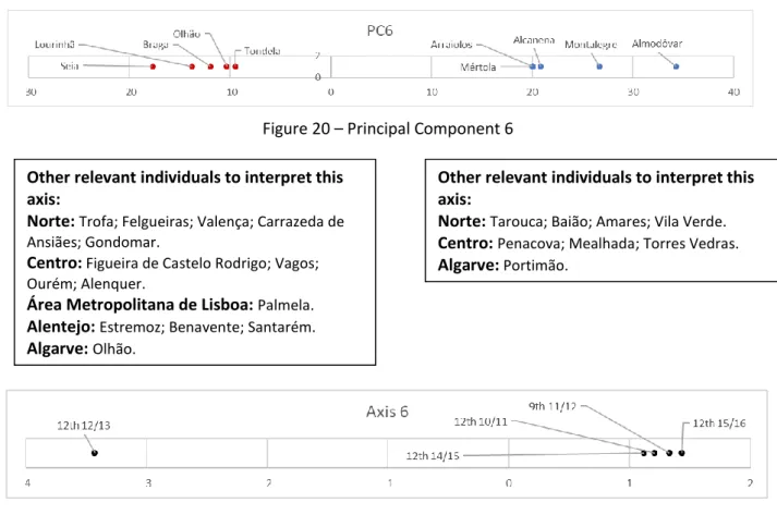
In this dimension, the municipalities that come across are the ones that have a higher/lower retention rate in 12th grade 2012/2013 than in the other variables that contribute the most to explain the inertia associated with this axis (12th 2010/2011, 2014/2015 and 2015/2016, and 9th grade 2011/2012). Nevertheless, much like in the previous component, there is only one variable that is well represented in this axis: 12th grade in 2012/2013.

In this case, Seia, Lourinhã and Braga, for example, have a higher retention rate in 12th grade in 2012/2013 than Almodôvar, Montalegre, and Alcanena.

What this shows is a very specific situation in this school year. If this is an exception, it might be interesting for the people responsible at the municipal level to identify the reasons behind the relative success or unsuccess achieved in this particular school year and level. Was it a specific group of students? An outstanding teacher?

(35)

23

Norte: Tarouca; Baião; Amares; Vila Verde.

Centro: Penacova; Mealhada; Torres Vedras.

Algarve: Portimão.

Norte: Trofa; Felgueiras; Valença; Carrazeda de Ansiães; Gondomar.

Centro: Figueira de Castelo Rodrigo; Vagos; Ourém; Alenquer.

Área Metropolitana de Lisboa: Palmela.

Alentejo: Estremoz; Benavente; Santarém.

Algarve: Olhão.

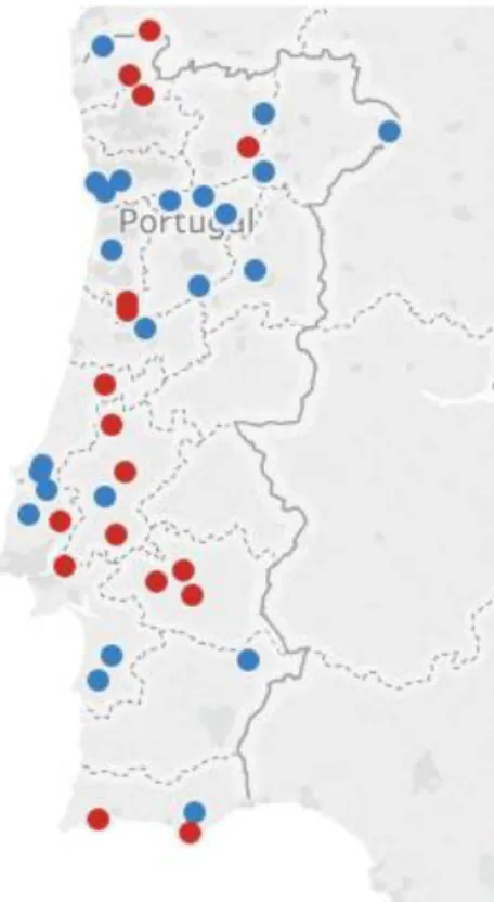
Here, there are interesting geographic trends to take into account. In the axis regarding principal component number 5, almost all the municipalities in the North of the country that was explained by that axis had a particularly high retention rate in 12th grade in 2013/2014. Now, the ones that are well explained in this one have a particularly high retention rate in 2012/2013. Valença is an example of a municipality that had high retention rates in both years. The same happens with Santarém, for example.

(36)

24

Norte: Baião; Porto; Felgueiras; Vila Verde; Valongo.

Centro: Celorico da Beira; Mealhada; Almeida; Penacova; Sabugal.

Norte: Ribeira de Pena; Vizela; Vila do Conde.

Centro: Proença-a-Nova; Figueira de Castelo Rodrigo; Pombal.

Alentejo: Odemira; Arraiolos; Viana do Alentejo.

Algarve: Silves.

4.1.7. Seventh principal component (PC7)

This seventh dimension represents 2.1% of the variance associated with the data.

The school years that contribute the most to explain the inertia associated with this axis are, on one side of the axis, 12th grade in 2010/2011 and 2015/2016, and 10th grade in 2015/2016. And, on the other, 10th grade in 2010/2011 and 9th grade in 2011/2012.

A closer look at the variables CTR shows very clearly that what is at stake in this component is the evolution of the retention rates in 10th grade from the beginning of the decade to 2015/2016. What it also shows is that, in certain municipalities, the retention rate was higher in 10th and 9th grade at the beginning of the decade than in 10th grade in 2014/2015 and 2015/2016. In some cases, the retention rates are even higher in 10th grade in 2010/2011.

The municipalities on the positive side of this axis have higher retention in 10th grade in 2010/2011 and improved in the last year under analysis. For the others, it worsened.

The municipalities better explained by this axis only explain 37% of the inertia associated with the axis.

(37)

25 Geographically, there is a clear predominance of municipalities on the negative side of the axis in the south of the country (in orange), shown in figure 25. While the ones located in the north (in blue) are mostly on the positive side. In spite of that, Almeirim and Coruche are the two municipalities in blue further south. Which means, again, that the variables that have improved are in the north. And then the municipalities with the worst performance (that get worse) are in the south.

There is, though, some clear oppositions between neighboring territories. That is the case with Ribeira de Pena and Vila Pouca de Aguiar and between Felgueiras and Vizela.

4.1.8. Eighth principal component (PC8)

This dimension represents 2% of the variance associated with the data.

What it is really at stake in this axis are the retention rates in 2012/2013 and 2013/2014 for 9th and 10th grade. The municipalities on the positive side of this axis peaked in retention rates in these years. The other ones had comparably lower retention rates.

The variables in the positive side of the axis represent the end of middle school and the beginning of high school, so we can say that the unsuccess is prolonged through the same level along the years but it also spreads to the next school level. This might mean that the students that had to repeat one level on 9th grade had to do it again on 10th grade but that is impossible to know (for now) because there is no information on individual students.

The municipalities that are better explained by this axis explain 43% of its inertia.

Figure 26 – Principal Component 8 Figure 25 – Geographic

distribution of the municipalities in PC7

(38)

26

Norte: Alfândega da Fé; Vale de Cambra; Lamego; Paredes; Valença; Baião; Vila Verde.

Centro: Cadaval; Sátão; Estarreja; Oleiros; Tábua.

Alentejo: Estremoz.

Centro: Cantanhede; Guarda; Penacova.

In this case, there is a very clear concentration of the municipalities better explained in this axis in the north of the country, and mainly by the sea.

Most of the municipalities here represented are on the positive side of the axis, meaning they have had high retention rates in 9th and 10th grade in the years under analysis. The exceptions are (from further south to the north), Lagos, Estremoz, Ponte de Sor, Cadaval and Peniche.

4.1.9. Ninth principal component (PC9)

This axis represents 1.9% of the variance associated with the data.

The high school years have controlled much of the analysis because it is, in fact, when the retention rates tend to increase. They are still present in this axis (the opposition between 12th grade in 2014/2015 and in 2015/2016) when we look at what variables best represent it. Nevertheless, the variables that are better explained by this axis are the ones regarding 9th grade as opposed to 7th grade in 2014/2015.

Figure 28 – Geographic distribution of the municipalities

(39)

27

Other relevant individuals to interpret this axis:

Norte: Terras de Bouro; Vieira do Minho; Vila do Conde.

Algarve: Lagoa.

Other relevant individuals to interpret this axis:

Norte: Vila Verde; Vila Nova de Gaia; Amares.

Centro: Tomar; Figueira de Castelo Rodrigo; Sabugal; Oleiros; Vila Nova de Paiva.

Área Metropolitana de Lisboa: Alcochete.

Alentejo: Ponte de Sor.

The municipalities better explained here – that explain 42% of the inertia associated with the axis - are either the ones who have a bigger retention rate in 7th grade 2014/2015 but lower in 9th grade (Celorico da Beira, Vagos, Cartaxo, for example). Or the other way around (Lagoa, Baião, Penafiel, for example).

In this dimension, there is also a clear geographical distribution. The municipalities that are on the negative side of the axis (in red) range from Lisboa to Viseu creating a diagonal line of places that are worse in 7th grade 2014/2015 than in the 9th grade, especially 2010/2011, 2012/2013 and 2013/2014.

But there are a few, the ones on the positive half (in blue) that are concentrated in Porto and Vila Real, as the figure 31 shows, that are worse in 9th grade than in 7th.

Figure 30 – Axis 9 Figure 29 – Principal Component 9

Figure 31 – Geographic distribution of the municipalities