Pesqui. Oper. vol.34 número1

A METHOD FOR SOLVING LINEAR PROGRAMMING MODELS WITH INTERVAL TYPE-2 FUZZY CONSTRAINTS

Juan Carlos Figueroa-Garc´ıa

_{and Germ´an Hern´andez}

Received December 20, 2012 / Accepted January 18, 2014

ABSTRACT.This paper shows a method for solving linear programming problems that includes Interval Type-2 fuzzy constraints. The proposed method finds an optimal solution in these conditions using convex optimization techniques. Some feasibility conditions are presented, and some interpretation issues are discussed. An introductory example is solved using the proposed method, and its results are described and discussed.

Keywords: Fuzzy Linear Programming, Interval Type-2 fuzzy sets, Fuzzy Optimization.

1 INTRODUCTION

Some practical applications such as financial, logistics, Markov chains, control, etc, include non-probabilistic uncertainty. This way, decision making has to deal with uncertainty using appropri-ate methods and models to find a solution of the problem. Linear Programming (LP) is within the most useful tools in decision making, and its application to non-deterministic problems has proved to be efficient (stochastic programming, fuzzy linear programming, etc). This opens the possibility of involving new uncertainty sources to problems where statistical information is not reliable or is absent through new theories such as fuzzy sets.

In some cases, availability of the resources of a system cannot be measured in an exact way (i.e. mathematical precision), due to different issues. Moreover, available information usually comes from the experts of the system, so decision making is intimately related to their perceptions and expertise. This information represents the knowledge of the experts about the availability of the resources of the system (a.k.a as constraints), which can be measured using fuzzy sets.

A special kind of LP models known as Fuzzy Linear Programming (FLP) models include fuzzy constraints. Roughly speaking, fuzzy constrained problems deal with non-probabilistic uncer-tainty, which is a common practical issue that needs special methods at different complexity levels.

*Corresponding author

1Universidad Distrital Francisco Jos´e de Caldas – Universidad Nacional de Colombia. 2Universidad Nacional de Colombia.

Some FLP models have been proposed by Ghodousiana & Khorram [8], Guu & Wu [9], Tanaka & Asai [29], Tanaka, Asai & Okuda [30], Inuiguchi & Ram´ık [11], and Inuiguchi & Sakawa [12, 13] who proposed solutions for several fuzzy sets, all of them considering only Type-1 fuzzy sets. An intuitionistic fuzzy optimization approach has been presented by Angelov [2] and Dubeyet al. [3], based on the idea of using two measuresµA(x)andυA(x)to represent both membership and non-membership degrees ofxregarding a concept A, constrained to 0 ≤ µA(x)+υA(x)≤1, which is similar to an Interval Type-2 fuzzy set in the sense that the distance betweenµA(x)and

υA(x)can be shown as an interval.

In this paper, we propose an extension of the FLP method proposed by Zimmermann [32, 33] (originally designed for Type-1 fuzzy constrained problems) to an Interval Type-2 FLP (IT2FLP) with linear membership functions. Our proposal uses Type-2 fuzzy numbers instead of pure intervals or intuitionistic fuzzy sets (even when they are uncertainty measures as well) to address non-probabilistic information coming from multiple experts.

The paper is divided into six sections. In Section 1, the Introduction and Motivation is presented. In Section 2, the classical LP model with fuzzy constraints is presented. In Section 3, some ele-ments of linguistic uncertainty, in particular Type-2 fuzzy constraints are introduced. In Section 4, a formal definition of an Interval Type-2 FLP model is provided, and Section 5 presents an optimization method. In Section 6, an illustrative application is introduced, and finally Section 7 presents some concluding remarks.

1.1 Motivation of using Type-2 FLP sets

Many decision making problems involve uncertainty, so the analyst has to deal with it (proba-bilistic and/or possi(proba-bilistic) in different ways. In LP problems, all its parameters (costs, tech-nological coefficients and constraints) can contain uncertainty, so different approaches can be used when different uncertainty sources appear. As usual, as more uncertainty sources are in-volved, more complex its modeling is (including the algorithms for finding a solution). A typical uncertainty source comes from the concept of a constraint, which is commonly assumed as de-terministic (in some cases, probabilistic). But, what if the constraints of the problem are defined by experts, or are they based on non-probabilistic information?

A specific kind of linguistic uncertainty can be considered when having experts’ judgements. This uncertainty appears when different perceptions of a concept are provided by different peo-ple, like the one arising when multiple experts (with equally valuable opinions) are defining the constraints of an LP problem. To do so, Interval Type-2 Fuzzy Sets (IT2FS) seem to be an ap-propriate representation of this uncertainty, so we propose its use to deal with the perception of multiple experts who define the constraints of an FLP problem.

2 THE ZIMMERMANN’S SOFT CONSTRAINTS MODEL

Zimmermann [32] and [33] proposed the following LP model which includes Type-1 fuzzy constraints:

max x∈X z=c

′_x+c 0

s.t.

Ax B (1)

x 0

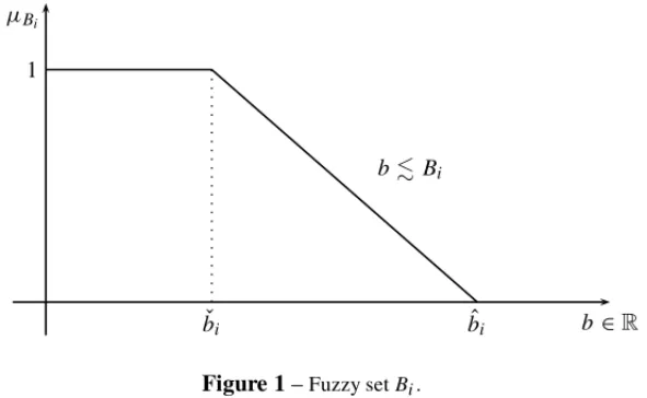
wherex,c∈ Rm_,c0 ∈ R, A ∈ Rn×m. Bis a vector ofi ∈ Nm fuzzy numbers, where a fuzzy number is a fuzzy set defined over the real numbers (see Fig. 1), andis a fuzzy partial order.1

N_{mis the amount of constraints of the problem.}

1

µBi

ˇ

bi biˆ b∈R

bBi

Figure 1–Fuzzy setBi.

Zimmermann proposed a method for solving this fuzzy constrained problem based on two re-quirements: B is defined as a vector ofN_{m L-R fuzzy numbers with linear membership}

func-tionsBi˜ ,i ∈N_{m, andB is characterized by a single membership function. B is defined by two}

parametersbˇi andbˆi (see Figure 1), and the remaining parameters are constants. The method is as follows:

Algorithm 1

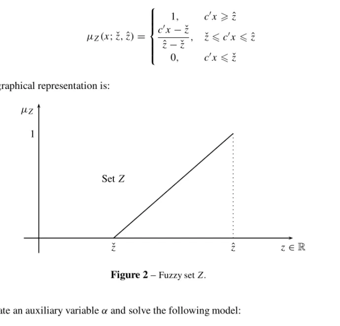
1. Define a fuzzy setZ with parameterszˇandz.ˆ

2. Computezˇ=max{c′x|Ax bˇ,x0}as lower boundary ofZ.

3. Computezˆ = max{c′x|Ax bˆ,x 0}as upper boundary ofZ. Given a maximizing goal, then the membership function ofZ(x)is:

µZ(x; ˇz,zˆ)=

⎧

⎪ ⎪ ⎪ ⎨

⎪ ⎪ ⎪ ⎩

1, c′xzˆ

c′x− ˇz

ˆ

z− ˇz , zˇc ′_{x zˆ}

0, c′xzˇ

(2)

Its graphical representation is:

1

µZ

ˇ

z zˆ z∈R

SetZ

Figure 2–Fuzzy setZ.

4. Create an auxiliary variableαand solve the following model:

max {α}

s.t.

c′x+c0−α(ˆz− ˇz)= ˇz (3)

Ax+α(bˆ− ˇb)bˆ x0, α∈ [0,1]

This method setsαas aglobal satisfaction degreeof all constraints regarding the fuzzy set of optimal solutions Z. In fact, α operates as a balance point between the use of the resources (denoted by the constraints of the problem) and the desired profits (denoted byz), since more resources usage imply higher profits, at different uncertainty degrees. Then, the main idea of this method is to find an overall satisfaction degree of both goals (profits vs. resource usage) that maximizes the global satisfaction degree,i.e.minimizing the global uncertainty.

Note that the set Z(x∗)represents the set of all optimal solutions regarding the goal. In other words, a thick solution of the fuzzy problem (see Kall & Mayer [14] and Mora [26]) where[ ˇz,ˆz]

3 INTERVAL TYPE-2 FUZZY CONSTRAINTS

As mentioned before, IT2FS allows to model linguistic uncertainty,i.e. the uncertainty about different perceptions and concepts. Mendel [15, 16, 18, 21, 24, 25] and Melgarejo [19, 20] provided formal definitions of IT2FS. Figueroa [4, 5, 6, 7] proposed an extension of the FLP which involves linguistic uncertainty using IT2FS called Interval Type-2 Fuzzy Linear Program-ming (IT2FLP). Some basic definitions include the following

3.1 Basics on interval Type-2 fuzzy sets

A Type-2 fuzzy set is a collection of Type-1 fuzzy sets into a single fuzzy set. It is defined by two membership functions: aprimary membership functiondefines the degree of membership over a linguistic label, and asecondary membership functionthat weights every Type-1 fuzzy set embedded into the primary function. According to Mendel [21, 22, 23], some basic definitions of Type-2 fuzzy sets include the following:

Definition 3.1 (Type-2 fuzzy set).A Type-2 fuzzy set,A, is:˜

˜

A=

x∈X

u∈Jx

fx(u)/(x,u)=

x∈X

u∈Jx

fx(u)/u x, (4)

wherexis theprimary variable, Jx is itsprimary membership function, Jx ⊆ [0,1],u is the secondary variableand_u∈J

x fx(u)/uis thesecondary membership function. Uncertainty about

˜

A is conveyed by the union of all of the primary memberships and is called theFootprint Of UncertaintyofA˜(FOU(A˜)),i.e.

FOU(A˜)=

x∈X

Jx (5)

Therefore, an FOU weights all the embedded Jx by using a secondary membership function fx(u)/u. In aGeneralType-2 fuzzy set(GT2FS), fx(u)/u is defined by a Type-1 membership function, while anInterval Type-2fuzzy set is a special GT2FS since its secondary membership function is 1 (one), fx(u)=1, as shown as follows

Definition 3.2 (Interval Type-2 fuzzy set).An Interval Type-2 fuzzy set,A, is:˜

˜

A=

x∈X

u∈Jx

1/(x,u)=

x∈X

u∈Jx

1/u x, (6)

The FOU ofA˜is bounded by two membership functions: anUppermembership function(UMF)

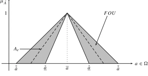
µ_A˜and aLowermembership function(LMF)µA˜. Note thatA˜has embeddedesets (Ae) as well, so there is an infinite amount of Ae enclosed into the FOU ofA. A graphical representation of˜ an IT2FS, its FOU andAeis shown in Figure 3.

Here, A˜is an IT2FS defined over a set,supp(A˜)∈ , its support2supp(A˜)is the support of

˜

A,supp(A˜)= [ ¯ˇa,a¯ˆ].µa˜ is a linear Type-2 fuzzy set with parametersa¯ˇ,a¯ˆ,aˇ,aˆ anda. FOU is theFootprint of UncertaintyofA, and˜ Aeis a Type-1 fuzzy set embedded on its FOU.

2_{is a compact set which represents the domain of the variablee.g. speed, height, etcn and usually it is defined as a}

Ae 1

µ_A˜

a ∈

¯ˇ

a aˇ a aˆ a¯ˆ

F OU

Figure 3–Interval Type-2 Fuzzy setA˜.

3.2 Uncertain constraints

There are many ways to define the“knowledgeability”of an expert, so an infinite number of Ae fuzzy sets can be comprised intoFOU(A˜). Each Ae is a representation of either the the knowledge of an expert aboutAor his perception about it. When multiple experts are defining a constraint, linguistic issues and multiple opinions about the same wordAdo appear, which is an uncertainty source itself.

Now we have defined what a Type-2 fuzzy set is, then an uncertain constraint can be defined as follows

Definition 3.3 (IT2FS Constraint – Figueroa [5]). Consider a set of constraints of an FLP problem defined as an IT2FS calledb defined on the closed interval˜ b˜i ∈ [bi,bi],{bi,bi} ∈R and i ∈N_m. The membership function which representsb˜iis:

˜

bi =

bi∈R

u∈J_bi 1/u

bi, i∈N_m, Jb_i ⊆ [0,1] (7)

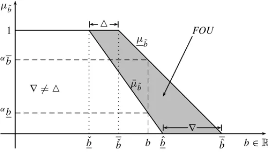
Note thatb˜is bounded by bothLowerandUpperprimary membership functions, namelyµ_˜

b(x) with parametersbˇandbˆandµ¯_b˜(x)with parametersb¯ˇandb. Now, the¯ˆ (FOU)of the setb˜can be composed by two distances called△and∇, defined as follows.

Definition 3.4 (Figueroa [5]).Consider an Interval FLP problem(IFLP)with restrictions in the form. Then△is defined as the distance betweenb andˇ b,ˇ △ = ˇb− ˇb and∇ is defined as the distance betweenb andˆ b,ˆ ∇ = ˆb− ˆb.

µ_˜

b

¯ µ_b˜ 1

µ_b˜

b∈R ˇ

b _bˇ bˆ _bˆ

α_b

α_b

b

FOU

△

∇ ∇ = △

Figure 4–IT2FS constraint with joint uncertain△&∇.

In Figure 4,b˜is an IT2FS with linear membership functionsµ_˜

bandµ¯b˜. A particular valuebhas an interval of infinite membership degreesu∈ Jb, as follows

Jb∈

α

¯ µb˜,

α

µ_˜

b

∀ b∈R ₍₈₎

where Jb is the set of all possible membership degrees(u)associate tob ∈ R_. αµ¯b˜ is theα -cut made over the upper membership function ofb, and˜ αµ_˜

bis theα-cut made over the upper membership function ofb, where the˜ α-cut of a fuzzy setbis defined asα_{b = {x|µ}

b(x)α}. Now, the FOU ofb˜can be composed by the union of all values ofu, as defined as follows

Definition 3.5 (FOU ofb˜).As defined in(8), it is possible to compose the footprint of uncertainty ofb˜,u∈ Jbas follows:

FOU(b˜)=

b∈R

α_µ¯ ˜ b,

α_µ ˜ b

∀ b∈ ˜b,u∈ Jb, α∈ [0,1] (9)

Remark 3.1. Definition 3.2 presents an L-R Type-2 fuzzy set as the union of all possible L-R Type-1 fuzzy sets into its FOU. Definition 3.3 defines an uncertain constraint as a monotonic decreasing Type-2 fuzzy set which represents the statement “Approximately less or equal than bi”. In this way, we refer to an uncertain constraint as the IT2FS defined in Definitions 3.3 and 3.2 with a membership function as displayed in Figure 4.

The problem of having a type-2 fuzzy constrained problem cannot solved in a closed form, so there is a need for finding an appropriate solution. Some interesting ideas about the concept of an optimal solution in terms of the decision variablesx∈R_{given uncertain constraintsb, can be}˜

points of a fuzzy set embedded into the FOU ofb, and then apply the Zimmermann’s method.˜ This method can be used in cases where the analyst has no a defuzzification criteria.

We have based our results in the Bellman-Zadeh fuzzy decision making principle, so the idea is to find a maximum intersection value between all constraints and Z. To do so, we need to provide some definitions of LP problems with IT2FS constraints in order to design a method for finding an optimal solution in terms ofx∈R_regardingzandb.˜

4 THE IT2FLP MODEL

Given the concept of an IT2FS constraint and the definition of an FLP, an uncertain constrained FLP model (IT2FLP) can be defined as follows:

max x∈X z=c

′_x+c 0

s.t.

Ax b˜ (10)

x0

wherex,c∈Rm_,c0∈R,A∈Rn×m.b˜is an IT2FS vector defined by two primary membership functionsµ

bandµ¯b.is a Type-2 fuzzy partial order.

Two possible partial ordersandcan be used depending on the problem. We use only linear membership functions since we are going to use LP models (easy to optimize using classical algorithms), which means less complexity. The membership function of(see Figure 4) is:

µ_˜

b(x; ˇb,bˆ)=

⎧ ⎪ ⎪ ⎪ ⎪ ⎨ ⎪ ⎪ ⎪ ⎪ ⎩

1, xbˇ

ˆ

b−x

ˆ

b− ˇb,

ˇ

bx bˆ

0, xbˆ

(11)

and its upper membership function (see Fig. 4) is:

¯

µ_b˜(x;b¯ˇ,b¯ˆ)=

⎧ ⎪ ⎪ ⎪ ⎪ ⎨ ⎪ ⎪ ⎪ ⎪ ⎩

1, xb¯ˇ

¯ˆ

b−x

¯ˆ

b−b¯ˇ

, b¯ˇx b¯ˆ

0, xb¯ˆ

(12)

A first approach for solving IT2FS problems is by reducing its complexity into a simpler form in order to use well known algorithms. In this case, we propose the following three-step methodol-ogy: 1– compute a fuzzy set of optimal solutions namelyz; 2– apply a Type-reduction strategy˜

to find a single fuzzy set Z; and 3– apply the Zimmermann’s soft constraints method to find a crisp solution. This allows us to see the above problem as the problem of finding a vector of solutionsx∈Rm_{such that:}

max x∈Rn

α

_m

i=1 { ˜bi, bi}

˜

z

whereαis theα-cut made over all fuzzy constraintsb˜iandz, defined as follows˜

µz˜(b˜)(z)= sup z=c′_x∗_+c

0

min i

µb˜i(x

∗_)|x∗_∈Rm ₍₁₄₎

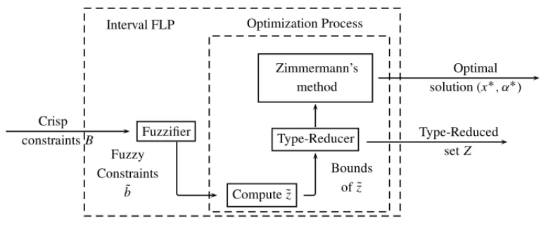
Givenµz_˜, the problem becomes in how to find the maximal intersection point betweenz˜andb,˜ whereαis an auxiliary variable. In practice, the problem is solved byx∗, soαallows us to find x∗according to (13). The proposed methodology for usingαoverz˜andb˜to findx∗is presented in Figure 5.

Crisp constraintsB

Fuzzy Constraints

˜ b

Bounds ofz˜ Fuzzifier

Compute˜z

Type-Reducer Zimmermann’s

method

Optimal solution (x∗, α∗)

Type-Reduced setZ Interval FLP Optimization Process

Figure 5–IFLP proposed methodology.

Figure 5 shows the three basic steps of our proposal: fuzzification, fuzzy optimization, and defuzzification. The main idea is to compute the fuzzy setZ˜ before applying a Type-reduction method for Type-2 fuzzy sets, to finally obtain a crisp solution using the Zimmermann’s soft constraints method. Now, there are two important conditions which ensures that an IT2FLP has an optimal solution in some point ofsupp(b˜):feasibilityandconvexitywhich are described next

4.1 Feasibility of an IT2FLP

An LP problem should befeasible. The concept of a feasible IT2FLP leads us to think that an IT2FLP should be feasible at every point ofb∈supp(b˜). In other words:

Proposition 4.1 (Feasibility of the IT2FLP).An IT2FLP is feasible iff the system

A(xi j)b¯ˆi ∀ i ∈Nm (15)

is feasible itself.

4.2 Convexity of an IT2FLP

Another important condition to be satisfied by any LP model isconvexity. In an LP problem, con-vexity means that the halfspace generated by allA(xi j)bshould be continuous and compact. This implies that every setbshould not be empty (non-null).

An IT2FLP has to guarantee two convexity conditions: a first one regardingb ∈supp(b˜)and a second one regardingµ_b˜. This leads us to the following proposition:

Proposition 4.2 (Convexity of an IT2FLP).An IT2FLP is said to be convex iff

A(xi j)b˜ ∀ i ∈N_{m (16)}

is a non-null halfspace, andb is composed by convex˜ µ_b˜andµ_˜

bmembership functions.

According to Kearfott & Kreinovich [17], global optimization is only possible for convex objec-tive functions, so the Proposition 4.2 agrees with this. Asz˜ is a function ofb, then we need to˜ guarantee thatµb˜be convex to ensure thatz˜be convex as well.

5 SOLUTION PROCEDURE OF AN IT2FLP

Until now our main problem is how to deal with interval fuzzy sets, since most of fuzzy opti-mization methods were designed for Type-1 fuzzy sets, and what we have is an interval of infinite choices. This way, our proposal is based on finding two endpoints enclosed into△and∇ (see Fig. 4), and use these points as the parameters of a single fuzzy set, suitable to be optimized using the Algorithm 1.

Figueroa [4, 5, 6] proposed a method to find an optimal fuzzy set embedded into the FOU of the problem using△,∇ as auxiliary variables weighted byc△andc∇ and the Zimmermann’s method. A description of the algorithm is presented next.

Algorithm 2

1. Compute an optimal inferior boundary calledZ minimum(ˇz)by usingbˇ + △as a frontier of the model, where△(see Definition 3.4) is an auxiliary set of variables weighted byc△ which represents the lower uncertainty interval subject to the following statement:

△b¯ˇ− ˇb (17)

To do so,△∗is obtained solving the following LP problem

max x,△ z=c

′_x+c

0−c△ ′△

s.t.

Ax− △bˇ (18)

2. Compute an optimal superior boundary calledZ maximum(ˆz)by usingb¯ˆ + ∇as a frontier of the model, where∇ (see Definition 3.4) is an auxiliary set of variables weighted byc∇ which represents the upper uncertainty interval subject to the following statement:

∇ b¯ˆ− ˆb (19)

To do so,∇∗is obtained solving the following LP problem

max x,∇ z=c

′_x+c

0−c∇ ′∇

s.t.

Ax− ∇bˆ (20)

∇ b¯ˆ− ˆb x0

3. Find the final solution using the third and subsequent steps of the Algorithm 1 using the following values ofbˇandbˆ

ˇ

b= ˇb+ △∗ (21)

ˆ

b= ˆb+ ∇∗ (22)

Remark 5.1 (Aboutc△andc∇).In Algorithm 2, we have definedc△andc∇as the weights of

△and∇. In other words,c_i△andc_i∇are the unitary cost associated to increase each resourcebˇ_i andbˆ_irespectively.

Remark 5.2 (max−minobjectives). The proposed algorithm was designed for maximization problems, so equations (21) and (22) apply to a max goal. For a min goal, equations (18), (20), (21) and (22) have to be changed.

Therefore, △and∇ are auxiliary variables that operate as Type-reducers3, where△∗_i and∇_i∗

becomebˇi andbˆi as the inputs of the Zimmermann’s method which returnszˇ∗,ˆz∗andα∗(see Section 2).

6 APPLICATION EXAMPLE

To illustrate how the proposed procedure works, we present a classical transportation problem where its demands and supplies are defined by the perception of the experts of the system in two fronts: experts of the behavior of the customer and experts of the suppliers’ capabilities.

Therefore, if different experts provide opinions based on their previous knowledge, the problem is how to handle the information they have provided. Sometimes, the experts provide opinions

3_{A Type-reduction strategy regards to a method for finding a single fuzzy set embedded into the FOU of a Type-2 fuzzy}

using words instead of numbers through sentences such as“I think that the demand of the product X should be between b1and b2”, whereb1andb2becomebiˇ andbiˆ, as presented in Section 1.

When different experts have different opinions for the same concept, then linguistic uncertainty appears and Type-2 fuzzy sets arise as an alternative to handle this kind of uncertainty. Is in that way how we present the demands and supplies of the system defined by the experts, where the main idea is to minimize the shipping costs of the system. A general IT2FLP transportation model is as follows:

minz=ci jxi j (23)

s.t.

−

m

i=1

xi j − ˜aj ∀ j∈Nn (24)

n

j=1

xi j di˜ ∀ i ∈N_{m (25)}

whereci j,xi j ∈Rn,m,a˜j andd˜i areIT2FS whose supports are defined over the real numbersR,

andare Type-2 fuzzy partial orders.

Index sets:

N_{mis the set of all}

“i′′resources,i ∈N_m,N_m =1,2, . . . ,m.

N_{nis the set of all “}j′′products, j∈N_n,N_n=1,2, . . . ,n.

Decision variables:

xi j= Quantity of product to be shipped from the supplier “i′′to the customer “j′′.

Parameters:

aj = Quantity of product available by the supplier “j′′.

di= Quantity of product required by the customer “i′′.

Note that b˜ (defined in (10)) is composed by two vectors: d˜ with parameters d¯ˇ,dˇ,dˆ anda,¯ˇ which are the demands of the customers, and a˜ with parameters a¯ˇ,aˇ,aˆ anda¯ˇ, which are the availabilities offered by suppliers.

Now, we need to computez˜andz∗=c(x∗)using (14),d˜,a˜andcwhich are provided as follows.

¯ˇ

di =

⎡ ⎢ ⎣ 10 11 12 ⎤ ⎥ ⎦ ˇ

d_i =

⎡ ⎢ ⎣ 13 14 18 ⎤ ⎥ ⎦ ¯ˆ

di =

⎡ ⎢ ⎣ 12 13 15 ⎤ ⎥ ⎦ ˆ

d_i =

⎡ ⎢ ⎣ 16 17 21 ⎤ ⎥ ⎦ ¯ˇ

aj =

⎡ ⎢ ⎣ 24 37 29 ⎤ ⎥ ⎦aˇj =

⎡ ⎢ ⎣ 16 30 23 ⎤ ⎥ ⎦a¯ˆj =

⎡ ⎢ ⎣ 20 32 24 ⎤ ⎥ ⎦aˆj =

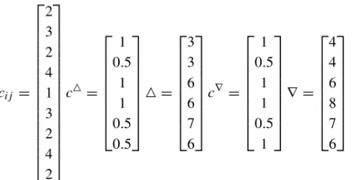
ci j = ⎡ ⎢ ⎢ ⎢ ⎢ ⎢ ⎢ ⎢ ⎢ ⎢ ⎢ ⎢ ⎢ ⎢ ⎢ ⎣ 2 3 2 4 1 3 2 4 2 ⎤ ⎥ ⎥ ⎥ ⎥ ⎥ ⎥ ⎥ ⎥ ⎥ ⎥ ⎥ ⎥ ⎥ ⎥ ⎦

c△=

⎡ ⎢ ⎢ ⎢ ⎢ ⎢ ⎢ ⎢ ⎣ 1 0.5

1 1 0.5 0.5

⎤ ⎥ ⎥ ⎥ ⎥ ⎥ ⎥ ⎥ ⎦ △ = ⎡ ⎢ ⎢ ⎢ ⎢ ⎢ ⎢ ⎢ ⎣ 3 3 6 6 7 6 ⎤ ⎥ ⎥ ⎥ ⎥ ⎥ ⎥ ⎥ ⎦

c∇ =

⎡ ⎢ ⎢ ⎢ ⎢ ⎢ ⎢ ⎢ ⎣ 1 0.5

1 1 0.5

1 ⎤ ⎥ ⎥ ⎥ ⎥ ⎥ ⎥ ⎥ ⎦ ∇ = ⎡ ⎢ ⎢ ⎢ ⎢ ⎢ ⎢ ⎢ ⎣ 4 4 6 8 7 6 ⎤ ⎥ ⎥ ⎥ ⎥ ⎥ ⎥ ⎥ ⎦

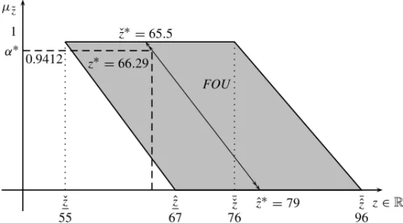
This example is composed by three suppliers and three customers whose parameters are defined by experts using IT2FS, so we apply the Algorithm 2 to find a crisp solution of the problem. The obtained fuzzy setZ˜ is defined by the following boundaries:

¯ˇ

z=76

¯ˆ

z=96

ˇ

z=55

ˆ

z=67

6.1 Obtained results

First, we have applied the LP models shown in (18) and (20), which lead to the following results:

△∗₁= 3 → dˇ₁∗= 10 ∇₁∗= 4 → dˆ₁∗= 12

△∗₂= 3 → dˇ₂∗= 11 ∇₂∗= 4 → dˆ₂∗= 13

△∗₃= 6 → dˇ₃∗= 12 ∇₃∗= 6 → dˆ₃∗= 15

△∗₄= 0 → aˇ₁∗= −16 ∇₄∗= 0 → aˆ₁∗= −14

△∗₅= 0 → aˇ₂∗= −30 ∇₅∗= 0 → aˆ₂∗= −25

△∗₆= 0 → aˇ₃∗= −23 ∇₆∗= 0 → aˆ₃∗= −18

Now, we use△∗and∇∗ alongside equations (21) and (22) to obtain the values ofzˇ∗ = 65.5 andzˆ∗ =79. Then, by usingdˇ,aˇ,dˆ,aˆ and the Zimmermann’s method we obtain the following results: α∗ = 0.9412 andz∗ = 66.29. The shipping quantitiesx_{i j}∗ that should be sent from suppliers to customers are shown next.

x₁₁∗ = 0 x₂₁∗ = 0 x₃₁∗ = 118.82

x₁₂∗ = 0 x₂₂∗ = 128.82 x₃₂∗ = 0

x₁₃∗ = 141.76 x₂₃∗ = 0 x₃₃∗ = 0.71

1 µ_˜z

z∈R ˇ

z 55

ˇ z∗=65.5

¯ˇ z 76

¯ˆ z 96 α∗

0.9412

ˆ z 67

ˆ z∗=79 z∗=66.29

FOU

Figure 6–Fuzzy setzembedded into the FOU ofZ˜.

6.2 Discussion of the results

We started to solve the problem with a set of constraintsd˜,a, in which we cannot make a shipping˜

decision. Then we applied the Algorithm 2 to obtain the endpoints△∗and∇∗which leads to

ˇ

d∗,aˇ∗,dˆ∗andaˆ∗. Finally we have applied the Algorithm 1 to find a crisp solution, which are in this case the optimal amount of demand to be satisfied, the amount of supplies to be used, and the shipping quantitiesx_{i j}∗ to be sent through the routei → j.

Note that our results depend onc△andc∇, so at a first glance, the method should not increase its delivering costs, but this does not happen as shown before. Moreover, the method decreases the satisfied demand, even by paying an additional costc△andc∇, plus shipping costs. Also note that△∗ _{= 0 and∇}∗ _{= 0 when the availability of suppliersa˜ is increased, since this leads to} increase its global shipping costs.

There is an interesting reason for: our method selects the constraints that increases the objective function, accomplishing (13) instead of the natural reasoning of treating all constraints in the same way.

Remark 6.1.Note that the presented example is feasible according to Propositions 4.1 and 4.2. This means that the problem is feasible sinced¯ˇ,a¯ˇare feasible points, and the problem is convex sinceµ_d˜andµ_d˜are linear convex membership functions, soZ˜as displayed in Figure 6 is convex as well.

Recall that our results are based on computingz¯ˇ,z¯ˆ,ˇz,ˆz,△∗_,∇∗_,zˇ∗_,zˆ∗_{which leads to a crisp} so-lution ofα∗,z∗andx∗_{i j}through LP models which can be solved using GAMS, LINGO, MatLab or any other optimization software. This provides a well known framework for further imple-mentations since there is no need for additional software and/or routines.

to be sentx_{i j}∗, accomplishing (13). This way, what we are doing here is making a decision using the Bellman-Zadeh fuzzy decision making principle.

7 CONCLUDING REMARKS

The proposed methodology (see Section 5 and Fig. 5) deals with Type-2 fuzzy uncertainty com-ing from the experts by uscom-ing well known fuzzy optimization techniques, achievcom-ing satisfactory results. Our proposal computes a fuzzy set Z˜ fromb˜before applying an optimization strategy, which is divided into two sub-steps: Type-reduction and defuzzification (performed by the Zim-mermann’s soft constraints method).

Our proposal uses the Zimmermann’s method for finding a crisp solution to a Type-2 constrained problem, so many similar problems can be solved using our proposal due to its flexibility and interpretability. Note that different Type-reduction strategies may be used, each one providing supplementary information for decision making.

Finally, the proposed methodology is a guide for handling Type-2 fuzzy constraints (involving the opinions and perceptions of different experts, their knowledge, and non-probabilistic uncer-tainty). Other methods can be used for (see Almeida, Yamakami & Takahashi [1], Silva, Cantao & Yamakami [28], and Hernandes, Berto & Castanho [10]), so our proposal is just an approach to solve this kind of problems.

REFERENCES

[1] ALMEIDATA, YAMAKAMIA & TAKAHASHIM. 2007. Sistema imunol´ogico artificial para resolver o problema da ´arvore geradora m´ınima com parˆametros fuzzy.Pesquisa Operacional,27(1): 131– 154.

[2] ANGELOVPP. 1997. Optimization in an intuitionistic fuzzy environment.Fuzzy Sets and Systems, 86(3): 299–306.

[3] DUBEYD, CHANDRAS & MEHRAA. 2012. Fuzzy linear programming under interval uncertainty based on ifs representation.Fuzzy Sets and Systems,188(1): 68–87.

[4] FIGUEROAJC. 2008. Linear programming with interval type-2 fuzzy right hand side parameters. In: 2008 Annual Meeting of the IEEE North American Fuzzy Information Processing Society (NAFIPS).

[5] FIGUEROAJC. 2009. Solving fuzzy linear programming problems with interval type-2 RHS. In: 2009 Conference on Systems, Man and Cybernetics, IEEE, pp. 1–6.

[6] FIGUEROAJC. 2011. Interval type-2 fuzzy linear programming: Uncertain constraints. In:IEEE Sym-posium Series on Computational Intelligence, IEEE, pp. 1–6.

[7] FIGUEROAJC & HERNANDEZ´ G. 2012. Computing optimal solutions of a linear programming prob-lem with interval type-2 fuzzy constraints.Lecture Notes in Computer Science,7208: 567–576.

[9] GUU S-M & WUY-K. 2002. Minimizing a linear objective function with fuzzy relation equation constraints.Fuzzy Optimization and Decision Making,1(4): 347.

[10] HERNANDESF, BERTONL & CASTANHOM. 2009. O problema de caminho m´ınimo com incertezas e restric¸ ˜oes de tempo.Pesquisa Operacional,29(2): 471–488.

[11] INUIGUCHIM & RAM´IKJ. 2000. Possibilistic linear programming: a brief review of fuzzy mathe-matical programming and a comparison with stochastic programming in portfolio selection problem. Fuzzy Sets and Systems,111: 3–28.

[12] INUIGUCHIM & SAKAWAM. 1994. Possible and necessary optimality tests in possibilistic linear programming problems.Fuzzy Sets and Systems,67: 29–46.

[13] INUIGUCHIM & SAKAWAM. 1999. A possibilistic linear program is equivalent to a stochastic linear program in a special case.Fuzzy Sets and Systems,76(1): 309–317.

[14] KALL P & MAYERJ. 2010.Stochastic Linear Programming: Models, Theory, and Computation. Springer-Verlag.

[15] KARNIKNN & MENDELJ. 2001. Operations on type-2 fuzzy sets.Fuzzy Sets and Systems,122: 327–348.

[16] KARNIKNN, MENDELJ & LIANGQ. 1999. Type-2 fuzzy logic systems.Fuzzy Sets and Systems, 17(10): 643–658.

[17] KEARFOTTRB & KREINOVICHV. 2005. Beyond convex? global optimization is feasible only for convex objective functions: A theorem.Journal of Global Optimization,33(4): 617–624.

[18] LIANGQ & MENDELJ. 2000. Interval type-2 fuzzy logic systems: Theory and design.IEEE Trans-actions on Fuzzy Systems,8(5): 535–550.

[19] MELGAREJOM. 2007. A Fast Recursive Method to compute the Generalized Centroid of an Interval Type-2 Fuzzy Set. In:Annual Meeting of the North American Fuzzy Information Processing Society (NAFIPS), IEEE, pp. 190–194.

[20] MELGAREJOM. 2007. Implementing Interval Type-2 Fuzzy processors.IEEE Computational Intel-ligence Magazine,2(1): 63–71.

[21] MENDELJ. 1994.Uncertain Rule-Based Fuzzy Logic Systems: Introduction and New Directions. Prentice Hall.

[22] MENDELJ. 2003. Fuzzy sets for words: a new beginning. In:The IEEE International Conference on Fuzzy Systems, pp. 37–42.

[23] MENDELJ. 2003. Type-2 Fuzzy Sets: Some Questions and Answers.IEEE coNNectionS. A publica-tion of the IEEE Neural Networks Society., 8 (2003), 10–13.

[24] MENDELJ & JOHNRI. 2002. Type-2 fuzzy sets made simple.IEEE Transactions on Fuzzy Systems, 10(2): 117–127.

[25] MENDELJ, JOHNRI & LIUF. 2006. Interval type-2 fuzzy logic systems made simple.IEEE Trans-actions on Fuzzy Systems,14(6): 808–821.

[26] MORAHM. 2001.Optimizaci´on no lineal y din´amica. Universidad Nacional de Colombia.

[28] SILVARC, CANTAOLA & YAMAKAMIA. 2012. Application of an iterative method and an evolu-tionary algorithm in fuzzy optimization.Pesquisa Operacional,32(2): 315–329.

[29] TANAKAH & ASAIK. 1984. Fuzzy Solution in Fuzzy Linear Programming Problems.IEEE Trans-actions on Systems, Man and Cybernetics,14(1): 325–328.

[30] TANAKAH, ASAIK & OKUDAT. 1974. On Fuzzy Mathematical Programming.Journal of Cyber-netics,3: 37–46.

[31] WOLSEYLA. 1998.Integer Programming. John Wiley and Sons.

[32] ZIMMERMANNHJ. 1978. Fuzzy programming and Linear Programming with several objective func-tions.Fuzzy Sets and Systems,1(1): 45–55.