HEURISTICS FOR IMPLEMENTATION OF A HYBRID PRECONDITIONER FOR INTERIOR-POINT METHODS
Marta Ines Velazco Fontova
1, Aurelio Ribeiro Leite de Oliveira
2*and Frederico F. Campos
3Received January 7, 2008 / Accepted April 15, 2011
ABSTRACT.This article presents improvements to the hybrid preconditioner previously developed for the solution through the conjugate gradient method of the linear systems which arise from interior-point methods. The hybrid preconditioner consists of combining two preconditioners: controlled Cholesky fac-torization and the splitting preconditioner used in different phases of the optimization process. The first, with controlled fill-in, is more efficient at the initial iterations of the interior-point methods and it may be inefficient near a solution of the linear problem when the system is highly ill-conditioned; the second is specialized for such situation and has the opposite behavior. This approach works better than direct meth-ods for some classes of large-scale problems. This work has proposed new heuristics for the integration of both preconditioners, identifying a new change of phases with computational results superior to the ones previously published. Moreover, the performance of the splitting preconditioner has been improved through new orderings of the constraint matrix columns allowing savings in the preconditioned conjugate gradient method iterations number. Experiments are performed with a set of large-scale problems and both approaches are compared with respect to the number of iterations and running time.
Keywords: Linear programming, Interior Point Methods, Preconditioning.
1 INTRODUCTION
Since the emergence of the interior-point method, sophisticated codes have been implemented in order to decrease the computational effort and improve its efficiency (Adler et al., 1989; Lustiget al., 1990; Mehrotra, 1992; Czyzyk et al., 1999). The most expensive step to each
*Corresponding author
1Faculty of Campo Limpo Paulista – FACCAMP, Rua Guatemala, 167, Bairro Jardim Am´erica, 13231-230 Campo Limpo Paulista, SP, Brazil. E-mail: [email protected]
2Instituto de Matem´atica, Estat´ıstica e Computac¸˜ao Cient´ıfica (IMECC), Universidade Estadual de Campinas (UNI-CAMP), Prac¸a S´ergio Buarque de Holanda, 651, Cx. Postal 6065, 13083-859 Campinas, SP, Brazil.
E-mail: [email protected]
iteration consists of the resolution of one or two linear systems. The most used approach for the solution of these systems is the Cholesky factorization (Golub & Van Loan, 1996), a procedure that may be expensive in large-scale problems.
An alternative for the solution of these systems is the use of iterative methods. The conjugate gradients method has shown to be the most efficient for the solution of the linear equations systems with large positive definite matrix.
To obtain the convergence of the iterative methods, it is fundamental to construct a preconditioner for the matrix of the linear system. These preconditioners should be easily built with relatively low computational cost and simultaneously, it should provide the convergence of the iterative method in a small number of iterations.
In this work, two specific preconditioners will be considered: controlled Cholesky factorization (Campos & Birkett, 1998) and the splitting preconditioner (Oliveira & Sorensen, 2005), pre-sented in Section 3.
Based on tests performed by Bocanegra et al. (2007) it has been proved that these two pre-conditioners determine a different behavior for the conjugate gradients method in the solution of the linear systems which arise from point methods. At the initial iterations of the interior-point method, the method of the conjugate gradients solves the linear systems involved more efficiently using the preconditioner obtained by the controlled Cholesky factorization (Campos & Birkett, 1998). At the final phase of the interior-point iterative process, where the linear sys-tems matrices are highly ill-conditioned, it was verified that the splitting preconditioner (Oliveira & Sorensen, 2005), specially developed for these systems, allows the conjugate gradients method to solve the systems in a quite efficient way.
This opposite behavior was availed by Bocanegra et al. (2007) developing a hybrid approach where both preconditioners are used for the solution of the linear systems in the same problem of optimization by interior-point methods. In the first phase of the optimization, the preconditioner obtained by the controlled Cholesky factorization is used, and in the second phase (final phase) the splitting preconditioner is used.
This work presents new heuristics to identify the moment in which the preconditioners change. Moreover, improvements to the efficiency of the splitting preconditioner are presented, con-sequently decreasing the number of iterations of the conjugate gradients method. The results are presented using large-scale problems and comparing the results with the ones obtained by Bocanegraet al.(2007).
2 PRIMAL-DUAL INTERIOR POINTS METHODS
A linear optimization problem may be presented in the standard form, as following:
min cTx
subject to Ax =b (1)
where A ∈ Rm×n is the matrix of restrictions withmrows andncolumns and rank(A)
=m,
c ∈ Rn is the vector of the cost of the problem, b ∈ Rn is the vector of the restrictions and
x ∈ Rn is the vector of variables of the problem, restricted to values which are non-negative
(x ≥ 0;xi ≥ 0,i =1,2, . . . ,n). Associated with the primal problem (1), the dual problem is
represented by:
max bTy
subject to ATy+z=c (2)
z≥0
wherey∈Rmis the vector of dual variables,z∈Rnis the vector of thegapvariablezrestricted
to non-negative values.
The primal-dual methods (Wright, 1996) solve the primal and the dual problems simultaneously from an initial point, not necessarily feasible, but strictly positive (interior point). The method is obtained from the application of the Newton’s method to the non-linear systemF(x,y,z) (Equa-tion 3) formed by the condi(Equa-tions of optimality, but not considering the non-negativity restric(Equa-tions:
F(x,y,z)=
Ax−b ATy+z−c
X Z e
=0. (3)
The Predictor-Corrector method (Monteiroet al., 1990; Mehrotra, 1992) is considered the most efficient approach for the solution of generic problems of linear programming.
This method uses three components to calculate the direction. A predictor direction 1x˜k,1y˜k,
1z˜kor the affine-scaling directions calculated from the system (4). This system of equations results from the Newton’s method applied to the system (3).
A 0 0
0 AT I Zk 0 Xk
1x˜k 1y˜k
1z˜k
=
b−Axk c−ATyk−zk
−XkZke
=
rkp rdk rak
=r. (4)
From the predictor direction, an auxiliary point is calculated x˜k,y˜k,z˜k,
˜
xk = xk+ ˜αp1x˜ ˜
yk = yk+ ˜αd1y˜ (5)
˜
zk = zk+ ˜αd1˜z
whereα˜pandα˜dare the steps calculated for the predictor direction, which guarantee the
interi-ority of the auxiliary point. The steps are defined as follows (Wright, 1996).
˜
αkp=min 1, α∙ min
∂xk i<0
− x
k i ∂xik
!!
,α˜dk=min 1, α∙ min
∂zk i<0
− z
k i ∂zki
!!
According to the predictor direction process, the disturbanceμkis calculated (Wright, 1996) μk = ˜
xkz˜k3
n xkzk2 sex kzk >1
xkzk2
n√n otherwise ,
and soon after that a direction of correction is computed. For this, the analogue system to the expression (4) (Mehrotra, 1992) known as Modified Newton’s method:
A 0 0
0 AT I Zk 0 Xk
1xk 1yk 1zk
=
rkp rdk rck
=
b−Ax˜k
c−ATy˜k− ˜zk μke−XkZke−1eXk1eZke
.
From the new direction, we calculate the next point in an equivalent way to (5).
It may be observed that in the predictor-corrector method, two linear systems at each iteration with the same matrix are solved.
The implementations of interior points work with matrices of lower dimensions obtained from the elimination of some variables.
If we use the third equation to eliminate1zwe obtain the augmented system (Equation 6) defined byD=X−1Z:
"
−D AT
A 0 # " 1x 1y # = "
rd−X−1 μe−Z e−1eX1eZ e
rp
#
. (6)
This system may still be reduced to a normal equations system by eliminating the1xvariable:
A D−1AT1y=A D−1 rd−X−1rμ
+rp. (7)
In the calculation of Newton’s directions, two linear systems involving the matrix A D−1AT are solved. For the solution of this system, direct methods may be used through Cholesky factor-ization or iterative methods. The most used iterative method is the preconditioned conjugate gradient.
In the next section, the hybrid preconditioner used for the preconditioning of the matrixA D−1AT
of the normal equation system (7) is presented.
3 PRECONDITIONERS
The preconditioning of a matrix is used to facilitate the convergence of iterative methods in the solution of linear systems.
Mehrotra (1992b) and (Lustiget al., 1990) define a preconditioner for the solution of linear systems by the conjugate gradient through the incomplete Cholesky factorization. The amount of zeros in the preconditioners is controlled and it highly influences the performance. The tests were carried out in the problems ofNetlib.
Wang & O’Leary (2000) developed a preconditioner for the solution of the linear system by an “adaptive” method. The method identifies when we should use the direct method and when we should use the iterative method by the preconditioned conjugate gradient. The initial precon-ditioner would be Cholesky factorization of the matrix generated in one of the iterations of the interior-point method. When thegap varies in the course of the iterations of the method, the preconditioner is calculated through up tonupdates of 1-rank according to the variation of the matrixD.
Bergamaschiet al. (2004) describe a preconditioner for the solution by iterative methods of the augmented system in the solution of problems of linear, non-linear and quadratic optimization. The preconditioner is calculated from Cholesky factorization of a new matrixAE−1ATwhere the matrixEis obtained from modifications made about the problem of optimization to have a more sparse factorization. When we use the complete factorization of the matrix as a preconditioner, the computational cost when the problem is linear is the same as when the direct method is used.
3.1 Hybrid preconditioner
The hybrid preconditioner (Bocanegraet al., 2007) is formed by the junction of two precon-ditioners: controlled Cholesky factorization and the splitting. The preconditioners are used in different phases of the process of optimization: controlled Cholesky factorization in the first phase and the splitting in the final phase where the system is very ill-conditioned.
3.2 Controlled Cholesky Factorization
The Controlled Cholesky Factorization (CCF) proposed by Campos and Birkett (1998) is a vari-ation of the incomplete Cholesky factorizvari-ation proposed by Jones and Plassmann (1995).
Being Q = A D−1AT and Qx = r the system of linear equations. Consider the complete Cholesky factorization ofQ =L LT and the incomplete factorization of Q =eLeLT +Rwhere
eLis an inferior triangular matrix obtained in the factorization and R, the remainder matrix. The matrixeL is used as preconditioner matrix. It is constructed from the selection of a fixed number of elements per columns with the largest absolute values.
DefiningE =L−eL, the controlled Cholesky factorization is based on the minimization of the Frobenius norm ofEgiven that whenkEk →0⇒ kRk →0. Consider the following problem:
minkEk2F = n
X
j=1 n
X
i=1
|li j − ˜li j|2= n
X
j=1
mXj+η
i=1
|li j − ˜li j|2+ n
X
i=mj+η+1 |li j|2
as:
n = order of the matrix;
mj = number of nonzero elements below the diagonal in the j-th column of the matrixQ; η = extra number of nonzero elements allowed per column.
The calculation of the norm is divided into two summations. In the first, we get the difference among the elements of the matrix L and the elements chosen which will form the matrixeL. The selected elements are the elements of the largest absolute values per column. The quantity selected is equal to the number of nonzero elements below the diagonal (mj)plus the extra
number of nonzero elements allowed per columns(η). In the second summation the difference is not realized, because in these positions the matrixeLwill have elements equal to zeros. Note that the higher the filling of the matrixeLthe lower will be its difference withL obtained by the complete Cholesky factorization.
The value ofηmay vary from−n ton. Whenηhas a positive value we will have a column j
with filling higher than the column jof the matrixQ. When the value is negative we will have a lower filling.
From tests carried out (Bocanegraet al., 2007), it has been proved that this factorization presents good results in the first iterations of the interior-point method, however it may deteriorates itself in the last ones, as the matrix Qgets very ill-conditioned.
3.3 Splitting preconditioner
The splitting preconditioner was proposed in (Oliveira & Sorensen, 2005) for the solution of the linear systems that arise from interior-point methods by iterative approaches, specifically by the conjugate gradient method.
The splitting preconditioner was originally developed for the augmented matrix of form:
−D AT
A 0
!
.
The final matrix preconditioned takes the form:
M−1 −D A T
A 0
!
M−T = −I+D
−1/2ATGT
+G A D−1/2 0
0 −DB
!
whereM is the preconditioned matrix and
M−1= D−
1/2 G
H 0
!
, G=HTD−B1/2B−1, H PT = [I 0] and A PT = [B N].
The preconditionerM may also be defined for the normal equations system. The matrixGmay be rewritten as:
G= A D−1AT =B DB−1BT +N D−N1NT. (8)
Multiplying byD−B1/2B−1and post-multiplying by its transpose in the Equation (8) we obtain the new preconditioned matrix:
D−B1/2B−1 A D−1ATB−TD−B1/2=I+D−B1/2B−1N D−N1NTB−TD−B1/2.
This preconditioner is more efficient near an optimal solution of the problem (4) when the linear system is highly ill-conditioned. In (Oliveira & Sorensen, 2005), the use of a diagonal matrix in the first iterations is proposed and the splitting preconditioner in the final phase of the optimiza-tion. This approach does not converge to many problems, because the diagonal preconditioner fails in many of them.
The highest computational cost in the calculation of this preconditioner consists of the construc-tion of the block B of the matrix A, wherem columns linearly independent are chosen. The way in which these columns are chosen is fundamental for the good performance of the pre-conditioner. The authors (Oliveira & Sorensen, 2005) suggest the choice of the firstmcolumns linearly independent of A D−1 with lower 1-norm. An advantageous property of this precon-ditioner is that the block B may be reused by several iterations making these iterations much cheaper.
3.4 Efficiency of the preconditioner
The splitting preconditioner builds a partition B of linearly independent columns and the way these columns are chosen influences its performance.
The authors (Oliveira & Sorensen, 2005) initially used the matrix D. New tests were carried out by the authors with the matrix A D−1, selecting the firstm linearly independent rows with lower 1-norm of the columns of this matrix. This new approach improved the performance of the preconditioner.
In this work, some problems have been tested using the ordering based onA D−1/2, the results did not show better performance. Using the matrixA D−3/2the performance of the preconditioner was improved with some problems.
We also propose a new ordering of the columns ofA D−1from the 2-norm. The firstmcolumns linearly independent of A D−1will be chosen with lower 2-norm kA D−1k2. This choice has
shown better results in the performance of the splitting preconditioner. The number of iterations of the conjugate gradient method in the solution of the linear system was reduced.
3.5 Change of preconditioner
The change of preconditioners is the fundamental point in the hybrid approach, because the efficiency of the preconditioners is very well defined in each phase of the optimization. However, each problem has a different behavior and consequently the phases are not easily identified. Bocanegraet al.(2007) realizes the change in the following conditions:
1. The initial GAP is reduced in 10−6and the number of iterations of the conjugate gradient is higher thanm/4 (mis the number of rows of the matrixA). It indicates that the process of optimization is very advanced and it may be the moment to change the preconditioner.
2. The number of iterations of the conjugate gradient in the solution of the linear system is nearm/2 (mis the number of rows of the matrixA). This may indicate that the controlled Cholesky factorization is not having a good performance.
3. If more than 10 corrections are made in the diagonal (which means that the matrix eL
was recalculated more than 10 times). In the construction of CCF, there may be non-positive pivots and to avoid this problem, a value is added to the diagonal (correction in the diagonal) and the matrixeLis recalculated.
If none of these three conditions is satisfied, then the η is increased by 10 and the method continues with the controlled Cholesky factorization.
In the study of this approach, it has been observed that these conditions are not always satisfac-tory. In all the tested problems, when a change of phase is realized very far from solution, the method does not reach the convergence.
In this way we verify that more coherent results are obtained when we use the controlled Cholesky factorization for the most number of iterations as possible. This new heuristic implies that the only condition that should be verified is the value of parameterη.
The new change of phase is realized when:
• If the iterations of the conjugate gradient are greater than m/6 then it is verified if η
reached a maximum value. If so, the change of the phases is realized, otherwise, ηis increased by 10 the process continues with the preconditioner obtained by the controlled Cholesky factorization. Note thatηis only used in the first phase.
For reasonable values ofηthe preconditioner obtained by the controlled Cholesky factorization is cheaper in its construction and requires less memory than the splitting preconditioner and therefore the highest number of iterations possible should be maintained. For some problems this approach fails, because very close to a solution the controlled Cholesky factorization can not work well. In the numerical tests presented in the following section these results will be verified.
4 NUMERICAL EXPERIMENTS
to solve the linear systems are written in the language C, with the exception of the code of the controlled Cholesky factorization which was implemented in FORTRAN. The same parameters of PCx were used with the exception of the multiple corrections that are not allowed.
4.1 Test problems
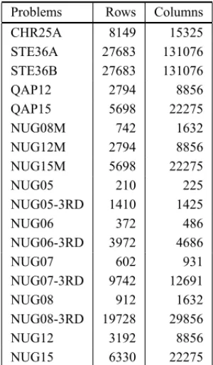
All the tested problems are of public domain. The QAP problems are from the QAPLIB library (Burkardet al., 1991) with the modifications described by Padberg and Rijal (1996). Some of the NUG problems were modified and the letter M, at the end of the name, was added as indicative. The Table 1 summarizes the problems tested showing the number of rows and columns after the preprocessing.
Table 1– Test problems data.
Problems Rows Columns
CHR25A 8149 15325
STE36A 27683 131076
STE36B 27683 131076
QAP12 2794 8856
QAP15 5698 22275
NUG08M 742 1632
NUG12M 2794 8856
NUG15M 5698 22275
NUG05 210 225
NUG05-3RD 1410 1425
NUG06 372 486
NUG06-3RD 3972 4686
NUG07 602 931
NUG07-3RD 9742 12691
NUG08 912 1632
NUG08-3RD 19728 29856
NUG12 3192 8856
NUG15 6330 22275
4.2 Computational results
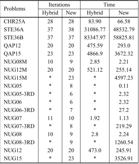
The performance of the hybrid approach proposed by Bocanegraet al. (2007) was compared with the performance of the new approach with the new condition of change of phases and the new ordering by the 2-norm. The results are summarized in Table 2.
Table 2– Comparison between the hybrid approach and the new approach.
Problems Iterations Time
Hybrid New Hybrid New
CHR25A 28 28 83.90 66.58
STE36A 37 38 31086.77 48532.79
STE36B 37 37 83347.97 58825.81
QAP12 20 20 475.59 293.0
QAP15 23 23 4866.9 3672.32
NUG08M 10 9 2.85 2.21
NUG12M 20 20 521.12 255.14
NUG15M * 23 * 4597.23
NUG05 * 8 * 0.11
NUG05-3RD * 6 * 2.32
NUG06 * 6 * 2.32
NUG06-3RD * 7 * 27.2
NUG07 11 10 1.92 1.13
NUG07-3RD * 8 * 219.29
NUG08 10 9 2.8 2.24
NUG08-3RD * 9 * 1260.54
NUG12 20 20 473.0 245.91
NUG15 * 23 * 3526.91
*: The method has not converged.
The initial value of ηin most of the problems was obtained from the average of the nonzero elements of the matrix A(Mel). In problems of higher scale as in the NUG15 the initialηis obtained adding 100 to the value of Mel. In general, the best time in the construction of CCF is obtained when we use the initial value of η = −Mel, but this approach did not have good performance for the bigger problems.
In most of the tested problems it was possible to decrease the computational time and for all of them the optimal was reached. The hybrid approach of Bocanegraet al. (2007) realizes the change of preconditioners in a stage in the process of optimization where the splitting precon-ditioner still does not obtain a good computational performance. The tests have shown that the best results are obtained when the CCF is used until the end of the optimization process.
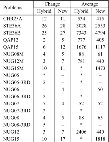
Table 3 shows the average of iterations realized using the new ordering by the 2-norm of the columns ofA D−1. The column “Change” shows the iteration where the change of precondition-ers was realized and the “Average” column shows the average of iterations carried out after the change.
of iterations of the conjugate gradient compared with the CCF, the use of the CCF for some more iterations continues to be more advantageous, due to the computational effort to calculateB.
Table 3– Comparison between the hybrid approach and the new approach in the change of preconditioners.
Problems Change Average
Hybrid New Hybrid New
CHR25A 12 11 534 415
STE36A 26 28 3028 2553
STE36B 25 27 7343 4794
QAP12 2 5 777 405
QAP15 6 12 1676 1117
NUG08M 4 5 88 61
NUG12M 3 7 781 440
NUG15M 10 11 * 1473
NUG05 * – * –
NUG05-3RD 2 – * –
NUG06 – 4 – 50
NUG06-3RD 2 – * –
NUG07 7 4 52 52
NUG07-3RD 2 – * –
NUG08 4 5 88 65
NUG08-3RD 5 – * –
NUG12 3 7 2406 440
NUG15 10 17 * 1818
*: The method has not converged; –: There was no change of preconditioner.
5 CONCLUSIONS
The problems presented in this work were tested by Bocanegraet al.(2007) using the PCx with the classic approach using direct methods for the solution of the linear systems. In most of the problems tested, it was possible to overcome the time of execution, the number of iterations and in some cases it was even possible to run new problems.
In this work, a new study of the hybrid approach applied to large-scale problems has been carried out. The study presents a new change of phase and a new reordering for the calculation of the matrixBof the splitting preconditioner.
The splitting preconditioner is very efficient in the last iterations of the interior-point method when the matrix Dobtained from the values ofxandzhas a well defined separation. The main point which defines the good operation is the choice of the columns which form the partition
B. The ideas developed in this work propose a new approach of ordering for the choice of this matrix that, as it has been shown, works better for all the problems tested. However, this ordering is not always respected, because from it the firstmcolumns linearly independent are chosen and it may occur that the last columns are part of the matrix B. This makes the construction of B
very expensive and still does not produce the expected results. Future works aim to improve this performance and eliminate these problems.
REFERENCES
[1] ADLERI, KARMARKARN, RESENDEMGC & VEIGAG. 1989. Data structures and programming techniques for the implementation of Karmarkar’s algorithm.ORSA Journal on Computing, pp. 84– 106.
[2] BERGAMASCHIL, GONDZIO J & ZILLI G. 2004. Preconditioning Indefinite Systems in Interior Point Methods for Optimization.Computational Optimization and Applications,28: 149–171.
[3] BOCANEGRAS, CAMPOSFF & OLIVEIRAARL. 2007. Using a hybrid preconditioner for solving large-scale linear systems arising from interior point methods.Computational Optimization and
Ap-plications(1-2): 149–164. Special issue on “Linear Algebra Issues arising in Interior Point Methods”.
[4] BURKARDRS, KARISCHS & RENDLF. 1991. QAPLIB – A quadratic assignment problem library.
European Journal of Operations Research,55: 115–119.
[5] CAMPOSFF & BIRKETTNRC. 1998. An efficient solver for multi-right-hand-side linear systems based on the CCCG(η)method with applications to implicit time-dependent partial differential equa-tions.SIAM J Sci Comput,19(1): 126–138.
[6] CZYZYKJ, MEHROTRAS, WAGNERM & WRIGHTSJ. 1999. PCx an interior point code for linear programming.Optimization Methods and Software,11(2): 397–430.
[7] GOLUBGH & VANLOANCF. 1996.Matrix Computations. Third Edition, The Johns Hopkins Uni-versity Press, Baltimore.
[8] JONES MT & PLASSMANN PE. 1995. An improved Incomplete Cholesky Factorization. ACM
Trans on Math Software,21(1): 5–17.
[9] LUSTIGIJ, MARSTENRE & SHANNODF. 1990. On Implementing Mehrotra’s Predictor-Corrector Interior Point Method for Linear Programming.TR SOR90-03.
[10] MEHROTRAS. 1992. On the Implementation of a Primal-Dual Interior Point Method.SIAM Journal
on Optimization,2(4): 575–601.
[11] MEHROTRA S. 1992b. Implementations of Affine Scaling Methods: Approximate Solutions of Systems of Linear Equations Using Preconditioned Conjugate Gradient Methods.ORSA Journal on
Computing,4(2): 103–118.
[12] MONTEIRORDC, ILANADLER& RESENDEMGC. 1990. A Polynomial-time Primal-Dual Affine Scaling Algorithm for Linear and Convex Quadratic Programming and its Power Series Extension.
[13] OLIVEIRA ARL & SORENSENDC. 2005. A new class of preconditioners for large-scale linear systems from interior point methods for linear programming.Linear Algebra and its applications, 394: 1–24.
[14] PADBERGM & RIJALMP. 1996.Location, Scheduling, Design and Integer Programming, Kluwer Academic, Boston.
[15] WANGW & O’LEARYDP. 2000. Adaptive use of iterative methods in predictor-corrector interior point methods for linear programming.Numerical Algorithms,25: 387–406.